AL: autogenerating supervised learning programs

AL: autogenerating supervised learning programs

The MIT Faculty has made this article openly available.

Please share

how this access benefits you. Your story matters.

Citation

Cambroner, Jose P. and Martin C. Rinard. “AL: autogenerating

supervised learning programs.” Proceedings of the ACM on

Programming Languages, 3, OOPSLA (October 2019): 175 © 2019

The Author(s)

As Published

10.1145/3360601

Publisher

Association for Computing Machinery (ACM)

Version

Final published version

Citable link

https://hdl.handle.net/1721.1/130326

Terms of Use

Creative Commons Attribution 4.0 International license

175

JOSÉ P. CAMBRONERO,

MARTIN C. RINARD,

We present AL, a novel automated machine learning system that learns to generate new supervised learning pipelines from an existing corpus of supervised learning programs. In contrast to existing automated machine learning tools, which typically implement a search over manually selected machine learning functions and classes, AL learns to identify the relevant classes in an API by analyzing dynamic program traces that use the target machine learning library. AL constructs a conditional probability model from these traces to estimate the likelihood of the generated supervised learning pipelines and uses this model to guide the search to generate pipelines for new datasets. Our evaluation shows that AL can produce successful pipelines for datasets that previous systems fail to process and produces pipelines with comparable predictive performance for datasets that previous systems process successfully.

CCS Concepts: · Software and its engineering → Automatic programming; · Computing methodologies → Machine learning.

Additional Key Words and Phrases: automated machine learning, program analysis for machine learning ACM Reference Format:

José P. Cambronero and Martin C. Rinard. 2019. AL: Autogenerating Supervised Learning Programs. Proc. ACM Program. Lang. 3, OOPSLA, Article 175 (October 2019),28pages.https://doi.org/10.1145/3360601

1 INTRODUCTION

Supervised learning has now become mainstream computing practice [Witten et al. 2016]. It has been successfully applied to solve problems as varied as identifying email spam, mapping gene expressions to diseases, and predicting stock returns [Borodin et al. 2004;Pantel et al. 1998;Tarca

et al. 2007]. Indeed, supervised learning is now widely applied across many areas of modern data

analytics and management.

A major challenge for analysts remains in effectively harnessing their experiences in prior modeling tasks and systematically applying these skills (and intuitions) to new tasks. Data analysts will frequently encounter new datasets and predictive tasks that require implementing new pipelines. Different datasets can require that the analyst perform different pre-processing (e.g. removing missing values) and choose different learning algorithms. We propose existing source code be analyzed and used to produce new supervised learning pipelines that emulate the work done by prior analysts, with little to no developer intervention or program annotation.

1.1 AL

Solutions to supervised learning problems often take the form of a sequence (pipeline) of calls to an API to 1) prepare the data for a learning algorithm through transformations, 2) apply a learning algorithm, and 3) evaluate the learned model on a held-out data set [Sparks et al. 2017]. More complex control flow beyond sequential composition is typically encapsulated in API components,

Authors’ addresses: José P. Cambronero, MIT, U.S.A, [email protected]; Martin C. Rinard, MIT, U.S.A, [email protected]. Permission to make digital or hard copies of part or all of this work for personal or classroom use is granted without fee provided that copies are not made or distributed for profit or commercial advantage and that copies bear this notice and the full citation on the first page. Copyrights for third-party components of this work must be honored. For all other uses, contact the owner/author(s).

© 2019 Copyright held by the owner/author(s). 2475-1421/2019/10-ART175

https://doi.org/10.1145/3360601

such as a static method that supports iteration over columns. For example, Scikit-Learn [Buitinck

et al. 2013] and XGBoost [Chen and Guestrin 2016], popular Python libraries often used together,

expose 51 classes and functions suitable for data transformations and 96 classes and functions for learning algorithms. The Scikit-Learn documentation on supervised learning algorithms alone is expansive (https://scikit-learn.org/stable/supervised_learning.html).

To use these libraries successfully, an analyst needs both knowledge of the components available in the libraries and machine learning expertise to identify relevant classes that work together well for the dataset and the prediction task at hand. Given the empirical nature of the prediction problem and the range of predictive performance across distinct pipelines, the developer will often experiment with different subsets and the composition order of the chosen components to construct candidate pipelines [Lee 2017;Tunguz 2018]. These pipelines are then evaluated to estimate future performance on unseen data.

We present AL, a system that learns to generate supervised machine learning pipelines from existing supervised learning programs. AL enables analysts to automatically obtain supervised learning pipelines for a wide range problems without the need to manually select the components in the pipeline or write code that implements the pipeline. AL identifies a sequence of components (in our evaluation, these are classes in two object-oriented machine learning libraries) that are appropriate for the input data. The system then adds additional boilerplate code necessary and returns a fully executable machine learning script to the user in plain Python code.

AL’s goal is to emulate the pipelines implemented in a collection of existing programs and provide a means to extend to new libraries with little to no additional development effort. By extracting the search space directly from a training set of programs, AL can automatically extend automated machine learning searches to new classes or functions used in the training set. This is a key advantage compared to existing systems that work with pre-defined subsets of libraries.

An analyst can use AL to generate new pipelines. To do so, the analyst provides AL with a dataset in tabular form. The columns correspond to features; each row is an observation. The user indicates which column of the table corresponds to the prediction target. AL then generates a set of pipelines consisting of method calls to API classes that process the input data, fit a learning model, and evaluate it. Each step in this pipeline takes as input the output of the previous step, and executes the API call with any remaining default parameters. The system outputs a ranked list of pipelines suitable for predicting the target value of new unseen observations.

1.2 Approach

We train AL on a collection of programs, each of which implement (potentially in addition to other functionality) a supervised learning pipeline. We source our training set of supervised learning programs from Kaggle [Google 2017a], a data science website that hosts competitions, tutorials, and community forums for relevant machine learning topics.

We train AL on a collection of approximately 500 supervised learning programs and their associated target datasets. AL instruments each program to collect runtime information. Specifically, the instrumentation collects a program trace, including information on the calls to the target machine learning libraries and an abstraction of the data used as parameters to those calls. The abstraction consists of a collection of feature functions that capture key characteristics (e.g. data types, summary statistics, probability densities, column correlations, missing value frequencies) of the input data to each call.

AL deploys a small set of module-level labels along with a slicing-based algorithm to extract a canonical representation of the supervised learning pipelines embedded in each dynamic trace. AL uses these canonical representations to construct a model to emulate developer-written pipelines. The model ranks candidate pipelines, based on the likelihood that a developer (as observed in

the training programs) would write such a pipeline. This model ranks new pipeline components conditioned on a partially constructed pipeline and the state of the input data presented to the new component. Given an input dataset, a pipeline depth bound, and a bound on the number of candidates per depth, AL uses the model to rank and prune candidate pipelines.

1.3 Results

We compare AL to two existing automated machine learning tools: Autosklearn [Feurer et al. 2015] and TPOT [Olson et al. 2016]. Both systems search over a space of preselected API classes, tuning the selection of classes used in the pipeline and their hyper-parameters. For our evaluation, we use AL to generate supervised learning pipelines for 31 data sets, none of which overlap with the data used by example programs seen by AL during training.

Our experiments show that by emulating existing pipelines, AL can produce pipelines for 18 out of 21 datasets in 5 minutes or less, with predictive performance comparable to those produced by existing systems, with the latter given a 1 or 2 hour execution budget (see Section9.3). We also show that by extracting the relevant API subset from programs, AL can eliminate the need to perform additional pre-processing of the data required by existing systems or remove the need to manually extend these systems by developers (see Section9.4).

1.4 Contributions

• AL: We present AL, a new automated machine learning system. To the best of our knowledge, AL is the first system to extract supervised machine learning pipelines from program traces and use these traces to learn how to generate pipelines for new data sets. This approach facilitates the use of existing ML knowledge captured in a collection of programs and the extension of automated machine learning searches to new libraries or libraries with extended APIs. Existing automated machine learning systems, in contrast, perform a search over preselected API components [de Sá et al. 2017;Feurer et al. 2015;Olson et al. 2016] and focus on choosing components for composition and optimizing the hyper-parameters associated with the chosen components. Current systems available need to be manually extended to consider new components for pipeline generation.

• Algorithm: We present the AL algorithm to extract supervised machine learning pipelines from programs, build a developer-emulation model from these pipelines, and employ this model to guide pipeline generation by ranking candidates.

• Experimental Results: We present results that demonstrate that automatic extension of the pipeline search space, through program analysis, can reduce the need to add handwritten-code to pre-process data. This approach also facilitates extending the search to new libraries. For 17 of 21 datasets in our evaluation, AL produces pipelines that perform comparable to existing automated ML systems. For 10 datasets, AL produces a pipeline when other AutoML systems fail to run.

The remainder of the paper is structured as follows. Section2walks through an example of how an analyst would use AL. Section3provides a brief overview of supervised learning and Section4

presents the idea of canonical supervised learning pipelines and estimating their likelihood. Section5

presents our algorithm for extracting the component search space and the canonical pipelines embedded in our training programs’ traces. Section6describes the process of collecting training programs. Section7details the use of a discriminative classifier to construct a developer-emulation model. Section8presents our pipeline generation algorithm. Section9shows our experimental results. Section10describes the AL implementation and provides a reference to a demo-version

repository with related code. Section11discusses threats to validity, Section12discusses AL in the context of previous work, and Section13presents future work. Section14concludes.

2 EXAMPLE

We next present an example that illustrates how AL produces a pipeline to solve a classification task for a new (unseen) dataset: the Titanic dataset [Kaggle 2015] hosted on Kaggle. The goal is to predict which passengers survived the Titanic wreck.

2.1 Training AL’s Pipeline Generation

We first train AL on a collection of supervised learning programs and their target datasets (in this paper these programs and datasets are sourced from the Kaggle website [Google 2017a]). AL collects dynamic traces from each program and extracts the canonical supervised learning pipeline embedded in each trace. It then uses these dynamic traces to build a probability model of pipeline likelihood conditioned on previous pipeline stages and on characteristics of the data at the current pipeline stage. AL uses this model to drive the exploration of candidate pipelines and produce candidates that emulate the pipelines written by developers and observed in the training programs. 2.2 Pipeline Generation

The dataset for the Titanic problem takes the form of a CSV file. Each row corresponds to a passenger. The columns correspond to passenger characteristics such as age, gender, cabin, etc. Starting with this file and an identification of the column name or index indicating the target prediction column, AL splits the file into a training dataset and a held-out validation dataset. It then runs its pipeline generation algorithm, using the conditional probability model to guide the search for good candidate pipelines (see Section8).

2.3 AL Pipeline

Figure1presents the highest ranked pipeline generated for the Titanic dataset. The pipeline consists of 3 classes from the Scikit-Learn library and a bounded loop iterator from AL’s runtime library, which are sequenced using Scikit-Learn’s Pipeline combinator, along with boilerplate code (which is generated by filling in a pre-defined sketch) to produce an executable machine learning pipeline. A Pipeline instance is constructed from steps, which are defined as a name and an operation and are applied in sequence to any inputs provided.

Lines 10 to 12 read the input dataset from disk and split the dataset into training and validation data. X_train and y_train correspond to the training data, and X_val and y_val correspond to the held-out validation dataset. The pipeline defines two transformations (lines 16 to 17), which are followed by fitting a logistic regression classifier (line 18). Line 22 fits each of these components in sequence, by calling .fit on the Pipeline instance. Line 25 evaluates the pipeline’s performance on the held-out validation set. To do so, the Pipeline instance’s .score method applies the transforms t0and t1 to X_val, predicts the outputs using the model, and compares these to y_val. Line 28 re-fits the pipeline to the entire dataset for training, so that new predictions can use all information available. The predict function (lines 30 to 31) produces new predictions for new data provided by the user.

The first component of the pipeline (line 16) is a class that applies a transform that converts strings into tokens, counts the number of times each token appears in each string, and replaces the string in the data set with columns that count the number of occurrences of each token. This transformation is required because the learning algorithm (line 18) works only with numeric data (and fails if presented with a dataset that contains text). Note that this class needs to be applied in a loop over the columns. Applying it to the table as a whole fails, as the API expects

1 i m p o r t x g b o o s t 2 i m p o r t s k l e a r n 3 i m p o r t s k l e a r n . f e a t u r e _ e x t r a c t i o n . t e x t 4 i m p o r t s k l e a r n . l i n e a r _ m o d e l . l o g i s t i c 5 i m p o r t s k l e a r n . p r e p r o c e s s i n g . i m p u t a t i o n 6 i m p o r t r u n t i m e _ h e l p e r s 7 8 from s k l e a r n . p i p e l i n e i m p o r t P i p e l i n e 9

10 # read i n p u t s and split

11 X , y = r u n t i m e _ h e l p e r s . r e a d _ i n p u t (' t i t a n i c . c s v ', ' S u r v i v e d ')

12 X_train , y_train , X_val , y_val = t r a i n _ t e s t _ s p l i t (X , y , t e s t _ s i z e =0 .25 )

13

14 # build p i p e l i n e with t r a n s f o r m s and model

15 p i p e l i n e = P i p e l i n e ([ 16 (' t0 ', r u n t i m e _ h e l p e r s . C o l u m n L o o p❶( s k l e a r n . f e a t u r e _ e x t r a c t i o n . t e x t . C o u n t V e c t o r i z e r❷) ) , 17 (' t1 ', s k l e a r n . p r e p r o c e s s i n g . i m p u t a t i o n . I m p u t e r❸() ) , 18 (' model ', s k l e a r n . l i n e a r _ m o d e l . l o g i s t i c . L o g i s t i c R e g r e s s i o n❹() ) , 19 ]) 20 21 # fit p i p e l i n e 22 p i p e l i n e . f i t ( X_train , y _ t r a i n ) 23

24 # e v a l u a t e on held - out data

25 print( p i p e l i n e . s c o r e ( X_val , y_val ) )

26

27 # train p i p e l i n e on train + val for new p r e d i c t i o n s

28 p i p e l i n e . f i t (X , y )

29

30 def p r e d i c t ( X_new ) :

31 r e t u r n p i p e l i n e . p r e d i c t ( X_new )

Fig. 1. Top ranked Python program generated by AL to perform classification on the titanic Kaggle dataset. The diagram displays the canonical pipeline implemented in the source code. AL populates predefined boilerplate code with the sequence of classes it chose to implement the pipeline. In this case, it chose a CountVectorizer

❷

❶

❸

❹

a one-dimensional vector to produce the appropriately shaped output. Removing string columns altogether would lose important information in the dataset such as gender or cabin class columns. Similarly, simply mapping each string to a unique integer would fail to extract relevant subtokens from string columns, such as passengers’ titles from the passenger name column (e.g. Miss, Mr, Master). Both of these features correlate with passenger survival [Elinder and Erixson 2012].

The second class in the pipeline (line 17) applies a transform that imputes missing data (filling in missing data with the mean over entries present in the same column). Again, this transformation is required because the learning algorithm fails if there is any missing data. Because this imputation class works only with numeric data, the pipeline also requires the previous application of a transform (such as the string to token count conversion transform in the example pipeline) that converts strings to numeric values. We highlight that the string to numeric conversion, and the filling in of missing values currently have to be handled manually when using previous systems (see

https://github.com/EpistasisLab/tpot/blob/master/tutorials/Titanic_Kaggle.ipynbfor an example

that uses this dataset with TPOT ). The removal of these manual steps underscores the advantages of learning from example programs as employed by AL.

All of the components in the pipeline, with exception of the custom combinator ColumnLoop in AL’s runtime library, were extracted from AL’s example supervised learning programs during

AL’s training. In each step, the input parameter to the API consists of the output from the previous pipeline step along with default parameters.

In practice, we expect that an AL user would automatically generate a set of pipelines, which they can choose to further modify by editing the pipelines’ Python source code. However, even an initial pipeline can deliver strong results, with no additional developer interaction. For example, as of this writing the AL pipeline in Figure1outperforms 91% of the submissions on the corresponding Kaggle leaderboard.

3 OVERVIEW OF SUPERVISED LEARNING

Let a dataframe be a collection of column vectors with potentially different datatypes. Let I be the set of dataframes with n rows and m columns. Let Y : Rn×1_{be the set of real-valued column vectors}

with n entries. Given I ∈ I and Y ∈ Y, supervised machine learning corresponds to building a hypothesis h (i.e., model) that maps each observation in I to the corresponding value in Y . This map is often constructed by minimizing a cost function over the predicted target values and the true target values for a portion of the data (training data). The expectation is that this map can generalize to unseen observations (test data).

It is often the case that the domain of Y is not the reals, but rather a discrete set of labels. When the domain of Y is a discrete set of labels, the problem is called a classification problem. When the domain of Y is the reals, the problem is called a regression problem. For brevity, we formalize the regression case, but a similar formulation for classification is possible.

4 CANONICAL SUPERVISED LEARNING PROGRAMS

We refer to a class, function, or method in an API that implements some desired functionality as a component. Let T : I → I be the set of, potentially stateful, components that transform dataframes to a space of dataframes with potentially different dimensionality and datatypes. We say we fit a transformation ti ∈ T on a dataframe X if we compute transformation parameters

from X and store these parameters in ti’s state. Let H : I → Y be the set of trained models

that take as input a dataframe and produce a vector of elements of the appropriate datatype. Let L: I × Y → H be the set of learning algorithm components that can train over an input dataframe and vector to produce a trained model. Let E : H × I × Y → R be the set of components that evaluate the performance of a trained model on held-out validation data and produce a model performance score.

Let Itrain,I_val ∈ Iand Y_train,Y_val ∈ Y. Let P represent the set of component-based programs implementing a supervised learning pipeline. A program in this set takes as inputs training data train = (Itrain,Ytrain)and held-out validation data val = (Ival,Yval). The program performs necessary

transformations to Itrain(and correspondingly, Ival), learns a model h ∈ H using train and evaluates

the performance of the learned hypothesis on val. The output of the program is the trained model and the associated evaluation metric on the held-out validation data.

A program in P is represented as a five tuple (train, val,T , l, e), where train is training data, val is held-out validation data, T = (t1, . . . ,t_k)is a sequence of k transformations where t_i ∈ T, l ∈ L is a supervised learning algorithm, and e ∈ E is an evaluation metric.

Figure2shows the evaluation semantics of such a program. We use Ii

trainto denote the output of

transformation ti on input I_traini−1, with I_train0 = Itrain. The output of this sequence of transformations is

used to learn a hypothesis over Ik

train,Ytrainusing the learning algorithm l. To evaluate the hypothesis

learned, we apply the same sequence of transformation components T , which may have computed parameters over Itrain(i.e. been fitted), to Ivaland use e to score the output of h(I_valk )relative to Yval.

Transform_ti(⟨Itrain,I_val⟩) → {I_train′ ← ti(Itrain); ⟨I_train′ ,ti(Ival)⟩}

ti(X ) → fit on X if unfitted and then transform else just transform

Learn_{l(Itrain,Ytrain) → model h on Itrain},Y_trainfit using algorithm l Evaluate_{e(h, Ival,Yval) → score trained model over validation data using e}

function Program(Itrain, Ytrain, Ival, Yval)

I_traink ,I_valk _{= Transform}tk(...Transformt0(⟨Itrain,Ival⟩)) h = Learnl(I_traink ,Y_train)

score = Evaluatee(h, I_valk ,Y_val)

return ⟨h, score⟩ end function

Fig. 2. Semantics for programs in P, the set of canonical supervised learning programs, where braces represent a program block, and a semi-colon represents operation sequencing. These programs produce a fitted hypothesis and a hypothesis score on held-out validation data.

4.1 Modeling Canonical Pipeline Likelihood

We model the conditional probability of a canonical supervised learning program (train, val,T , l, e) ∈ Pas the probability that a developer would write the sequence of operations t1, ...,tk,l, given the training data. This probability model can be viewed as a łlanguage modelž over pipelines, conditioned on input data [Rosenfeld 1996]. This intuition captures our goal: developer emulation during pipeline generation. We remove the evaluation component from the likelihood calculation as the function used to score a pipeline is defined deterministically based on the prediction task, to allow comparison of multiple pipelines’ performance. The probability is then defined as:

Pr(T , l |Itrain,Ytrain) =

Pr(l |T , Itrain,Y_train)

k

Y

i=1

Pr(ti|T1i−1,Itrain,Y_train) where T_ij indicates the sequence ti. . .tj, and T∗0is the empty sequence.

We approximate this distribution by making a Markov assumption [Baum and Petrie 1966] of order j about the transformations and learning algorithm in the program. This assumption is that the ith pipeline component is a function of only the j previous calls and the input data before the ith call. By considering the input data for the ith call, rather than the initial data, we allow some additional information flow beyond the cutoff imposed by our Markov assumption. So our approximate conditional probability distribution is

∝Pr(l |T_{k −j}k ,I_traink ,Y_train) k Y i=1

Pr(ti|T_i−ji−1,I_traini−1,Y_train). (1)

4.2 Abstracting Inputs for Learning

To estimate the conditional probability distribution defined in Equation (1), we need a data abstrac-tion that is flexible across different inputs. This flexibility must account for varying dimensions, datatypes, and underlying distributions. We define such an abstraction operation α : I ∪ Y → Rp

which summarizes input data using a real-valued vector of dimension p. The vector is designed to capture key characteristics of the data. We often refer to the application of α as summarizing the input.

Using α , we cast the problem of learning the conditional probability distribution for super-vised learning problems as a supersuper-vised learning problem itself, an approach known as meta-learning [Giraud-Carrier et al. 2004]. We consider each transformation ti or learning algorithm l as

a label, and train a discriminative classifier to predict the appropriate label given the previous j pipeline components and the current call’s input data.

The feature map that defines α presents a trade-off between the richness of the representation, sparsity in training data, and computational cost. Producing very rich representations reduces the likelihood that we will observe many instances of the vector in our training data, and may be more expensive to compute during pipeline search. Very simple representations can fail to capture important features of the input data. Based on our own experience and the existing literature [Ali

and Smith-Miles 2006;Reif et al. 2014], we define α using the following combination of features,

which are averaged column-wise where relevant. Probability/cumulative density functions used are defined with a set of fixed distribution parameters and applied to each value in a column.

• Type Features: Collection type (e.g. list, array, set); distribution of types in collection ele-ments (e.g. real, integer, string).

• Features for Numeric Data: Arithmetic mean; Geometric mean; Median; Minimum; Maxi-mum; Maximum and minimum of z-score; Interquartile range; Skew; Kurtosis; Maximum and minimum of probability density function evaluation under normal, chi-squared, exponential, and gamma distributions; maximum and minimum of cumulative density function evaluation under normal, chi-squared, exponential, and gamma distributions; correlation; Count of missing values.

• Features for Categorical Data: Size of domain; Minimum, maximum, and mean frequency of elements in domain; Count of missing values.

Table1compares the features used in computing α with the features used by Autosklearn in its meta-learning.

5 EXTRACTING A COMPONENT SEARCH SPACE

Our system eliminates the need to manually select a set of relevant API components for constructing a supervised learning pipeline. This approach relies on dynamic program traces collected by executing existing supervised machine learning programs. We focused on Python programs that contained calls to two popular data science libraries: Scikit-Learn [Buitinck et al. 2013], and XGBoost [Chen and Guestrin 2016].

The program traces, collected through dynamic instrumentation, contain the API calls made by the program along with information on the arguments and memory locations associated with each call. We describe the details of our instrumentation in Section6.1. To extract a canonical pipeline from such a trace, we need to label each call as an element in T , the set of available transformations, L, the set of available learning algorithms, or E, the set of available evaluation functions.

The sets of calls for each of the three labels are then used to train a model that predicts the likelihood of observing a particular component, given prior components and the state of the input data. For example, we collect all calls labeled T and train a model that predicts the likelihood of observing a given transformation component, such as sklearn.preprocessing.Imputer, next in the pipeline.

Table 1. Comparison of data features used in Autosklearn’s meta-learning and AL’s α

Meta-Feature Autosklearn AL

Class entropy ✓ ✗

Class probability (max, min, mean, std) (max, min, mean) Ratio of rows to columns ✓ ✗

Kurtosis (max, min, mean, std) mean Number of columns ✓ ✓

Number of rows ✓ ✓

Number of features by type ✓ ✓ Number of classes ✓ ✓ Ratio of feature types ✓ ✗ Skewness (max, min, mean, std) mean

Symbol counts (max, min, mean, std, sum) (max, min, mean) Count of rows with missing values ✓ ✗

Count of features with missing values ✓ ✗ Percentage of missing values ✓ ✓

Cross-column correlation ✗ (max, min, mean) Non-zero counts ✗ (mean)

PDF/CDF for common distributions ✗ (normal, chi2, exponential, gamma) Other summary stats ✗ (geometric mean, median, zscore, IQR, std)

5.1 Dynamic Trace Slicing For Canonical Program Extraction

Algorithm1presents how we 1) label each API call in a dynamic trace, and 2) extract a canonical supervised learning program. We exploit the package hierarchy in Scikit-Learn and XGBoost’s bindings to label as an element of T any function or appropriate method call for a class defined in Scikit-Learn’s decomposition, feature_extraction, feature_selection, pipeline, preprocessing, and random_projection modules.

Similarly, we label as an element of E any function or appropriate method call for a class defined in Scikit-Learn’s calibration, metrics, model_selection modules. We also use the fact that all learning algorithms in Scikit-Learn and XGBoost’s Python bindings are implemented as classes with a fit method to apply the respective learning algorithm to data. We identify all calls to fit that are not already labeled and label these as elements in L.

We say that a call that has been labeled as an element in L is a seed for a canonical supervised learning program. There may be multiple seeds in a single dynamic trace, yielding multiple canonical programs. For each seed in the trace, we slice the trace forward using the data dependencies on the seed call’s return value to identify calls that depend on the output of that seed. These calls are labeled as elements of E, if not previously labeled. We then slice the trace backwards using the data dependency information for the seed call’s parameters to identify calls that are inputs to the learning algorithm. These calls are labeled as elements of T , if not previously labeled. Concatenating the backward slice, the seed, and the forward slice produces a canonical program.

Call labeling in a canonical program is done on a per-example basis. This means that a single method on the same class can be labeled differently across different example programs. This approach provides AL with additional flexibility. The dynamic slicing-based labeling also allows users to provide an incomplete set of method/class labels, which can be supplemented with labels assigned during slicing. This approach reduces the annotation burden for adapting AL to new APIs. It is important to note that the traces we extract are a linearization of the original slice. So for example, if the slice contains two transforms A and B with edges into learning algorithm C, the linearized trace extracted would correspond to A, B, C, where A and B have are placed in an

arbitrary (deterministic) order. This linearization is a direct result of our pipeline language model, which is restricted to characterizing pipelines with sequential transformations.

Figure3shows an example canonical pipeline extracted from our training data. Each component is labeled according to its role in the pipeline. T stands for transform, L stands for learning algorithm, and E for evaluation.

Algorithm 1 Extract canonical supervised learning programs from a dynamic program trace. Each call is labeled as part of T (T ), L (L), or E (E)

INPUT: D, a dynamic trace; P , a limited set of predefined mappings from API calls to labels. Let SliceFWD_{(d, s) and SliceBWD(d, s) respectively, compute a forward and backward slice on} dynamic trace d starting from call s using data dependencies.

OUTPUT: A set of labeled canonical supervised learning programs from a single trace.

1: function Canonical-Prog(D, P )

2: progs ← ∅

3: Label subset of calls in D using P

4: ▷Seeds correspond to calls fitting a learning algorithm

5: seeds ← {call ∈ D|call.label = l ∨ (call.label = None ∧ call.method = .fit)}

6: for s ← seeds do

7: s.label ← L

8: bwd ← SliceBWD(D, s)

9: Label calls in bwd as T if not previously labeled

10: fwd ← SliceFWD(D, s)

11: Label calls in fwd as E if not previously labeled

12: prog ← Concatenate(bwd, seed, fwd)

13: progs ← progs ∪ prog

14: end for

15: return progs

16: end function

6 COLLECTING TRAINING DATA

We collected and analyzed a set of supervised learning programs crowdsourced through Kag-gle [Google 2017a], a data science website that hosts machine learning competitions, datasets, tutorials, and forums. Users are provided with an extensive environment to write and execute their own scripts in popular data science languages such as Python and R, with access to Kaggle’s datasets. We used Kaggle’s Meta-Kaggle dataset [Kaggle 2017], which includes existing user scripts. We downloaded the input data for these programs, and used this data to reproduce program executions. We learn from Python programs that made at least one call to our target libraries: Scikit-Learn and XGBoost [Chen and Guestrin 2016]. Both libraries are used in existing automated machine learning tools [de Sá et al. 2017;Feurer et al. 2015;Olson et al. 2016] and were used often in Kaggle scripts. We removed scripts that exceeded a predefined similarity ratio over token subsequences [Ratcliff

and Metzener 1988]. This filtering aims to remove scripts that have few semantic differences.

These łduplicatesž are often produced as a result of the ad-hoc version management common in data science development [Kery et al. 2017]. Our final training set consisted of approximately 500 programs from the Meta-Kaggle dataset. These programs solved one of 9 problems (meaning they perform predictions over 9 different datasets).

[(' T f i d f V e c t o r i z e r ', 'T ') , (' T f i d f V e c t o r i z e r . f i t ', 'T ') , (' T f i d f V e c t o r i z e r . t r a n s f o r m ', 'T ') , (' T f i d f V e c t o r i z e r . t r a n s f o r m ', 'T ') , (' T r u n c a t e d S V D ', 'T ') , (' T r u n c a t e d S V D . f i t _ t r a n s f o r m ', 'T ') , (' T r u n c a t e d S V D . t r a n s f o r m ', 'T ') , (' S t a n d a r d S c a l e r ', 'T ') , (' T r a n s f o r m e r M i x i n . f i t _ t r a n s f o r m ', 'T ') , (' S t a n d a r d S c a l e r . t r a n s f o r m ', 'T ') , (' R a n d o m F o r e s t C l a s s i f i e r ', 'L ') , (' B a s e F o r e s t . f i t ', 'L ') , (' F o r e s t C l a s s i f i e r . p r e d i c t ', 'E ') ]

Fig. 3. A canonical pipeline extracted from an existing program trace during AL’s training. Each tuple consists of a call and a component label. This pipeline uses TfidfVectorizer to convert strings to counts and normalize them, TruncatedSVD to perform dimensionality reduction, StandardScaler to scale the reduced data, and RandomForestClassifier to fit a classifier.

6.1 Program Instrumentation

To obtain program traces from which to learn, AL uses dynamic instrumentation. The goal of this instrumentation is to identify key execution events (particularly, assignments, calls and returns) to maintain a simplified data flow graph, which we refer to as a value graph. Nodes in the value graph are created based on execution events and annotated with data to allow trace extraction.

To effectively instrument the program, AL first performs multiple rewrites. In particular, any function (or method) call is hoisted such that it assigns to a fresh intermediate variable, and the corresponding call in the original statement is replaced with the intermediate variable. Then AL adds calls to its instrumentation runtime library, which maintains information, detailed below, during execution. We now detail the actions taken by the instrumentation for key events. Assignments: When an assignment executes, AL records a new node in the value graph for each left-hand-side variable. To record data dependences, AL extracts all variables used on the right hand side of the assignment and adds a directed edge from the latest graph node associated with that variable to the new nodes just created. If there are no variables on the right-hand side (e.g. the assignment is a constant expression), no dependences are added. To identify the appropriate node for each variable, we rely on their memory address, which can be obtained in CPython by the

idfunction. The instrumentation uses the memory address as a key into a hash table containing graph nodes. Finally, the newly created graph nodes are stored in the slots associated with the corresponding value ofidfor each left-hand-side-variable.

Calls: When a call executes, AL records a new node in the graph with an identifier for the call site, an identifier for the particular call, source code information and any arguments used for the call. For each variable used in a call argument, AL adds a directed edge from the node associated with the last assignment to that variable to the new call node. The call node created also includes a summary of each call argument, produced using the output of AL’s data abstraction function.

In contrast to a more general data flow analysis, we highlight that for AL we have the advantage of only caring about calls to a subset of libraries in each program (Scikit-Learn and XGBoost). Caring about a smaller subset reduces the calls that have to be instrumented, and given their standard usage patterns, allows us to simplify instrumentation, for example by eliding instrumentation for

more complex Python constructs like generators, conditional expressions, lambdas, among others. This may result in incomplete value graphs, but we have not found this to impact AL’s performance. Returns: When a return event occurs, AL adds a new node for the return and creates an edge from the node associated with the corresponding call to the current new node. If the return value is further assigned to a variable (as is often the case, given that we hoist calls), the following Assignment execution event handles the remainder of the necessary value-graph updates. Loops: Iteration in example programs can unduly affect AL’s language model. For example, if a program iterates over each row of a table and applies a particular transformation T , our probability for T would be biased by the number of rows in that table. This behavior would also violate the defined semantics of transformations, which apply to a table as a whole not to a row, leading to an incorrect probability computation. To resolve this issue, AL adds a static identifier to each for and while loop in the original program, as well as a dynamic identifier assigned when a for or while loop body is entered during execution. AL then only records events in the body of the loop during the first iteration associated with the current dynamic identifier, effectively unrolling the loop once for instrumentation purposes during execution. AL keeps track of the corresponding dynamic and static identifiers for that loop, such that a new entrance in the body of the loop (e.g. a new call to a function that contains the loop in question) would once-again produce nodes for the value graph. After a program has finished executing, we post-process the value graph to facilitate extraction of program traces. Specifically, AL extracts call nodes and merges edges as necessary, so that our final graph contains an edge from call A to call B if the return value of A flows into B, with no intermediate function C modifying A’s return value.

We encapsulated these ideas in an instrumentation library,https://github.com/josepablocam/

python-pl, that relies on the Python debugger to carry out the instrumentation tasks outlined

previously. This library uses a combination of source code and runtime type information to identify calls to functions in its own code, relevant libraries (i.e. those we want to track) and irrelevant libraries. It also disambiguates between calls made from the input program and calls that may be internal to libraries (which we do not care for, as AL focuses on public API components). The current version of AL is implemented with the same general approach, but relies more heavily on inserting calls to the runtime instrumentation library in the rewritten source code.

7 A DISCRIMINATIVE CLASSIFIER FOR SUPERVISED LEARNING PROGRAMS We use multi-label logistic regression with L1regularization, a standard machine learning algorithm,

to model the conditional probability distribution of supervised learning pipelines.

Recall that in Equation (1) we defined the conditional probability of a canonical supervised learning program as proportional to

Pr(l |Tk k −j,I k train,Ytrain) k Y i=1

Pr(ti|Ti−ji−1,Itraini−1,Ytrain) (2)

which has a Markov assumption of order j.

We instantiated j to 2 in our implementation, which means our model considers only the two previous pipeline operations, along with the input to the current operation, when computing the probability of the next component. In order to choose j, we performed k-fold cross validation over next-component prediction. A new set of training programs would potentially require a different j, but this new j value can be determined empirically using a similar approach.

We also abstract out the input data using our α data summarization function. We trained two separate classifiers: one for transformations and one for learning algorithms. Let PrT be the

Fig. 4. Graphical representation of our language model

conditional probability computed by the former classifier, and PrLbe the conditional probability

computed by the latter classifier.

We then redefine the (unnormalized) conditional probability for a supervised learning program to

PrL(l |tk −1,t_{k −2},α (I_traink ), α (Y_train)) k

Y i=1

PrT(ti|ti−2,ti−1,α (I_traini−1), α (Y_train))

We summarize this model through a simple graphical representation, shown in Figure4. We consider the previous two pipeline components (tj−2 and tj−1) and a summary of the current

state of the dataset (i.e. the input into the next pipeline component, α (I_{t r ain}j−1 ) and α (Yt r ain)). The

corresponding model then predicts the probability for the next transformation (PrT) or learning

algorithm (PrL).

We trained the two classifiers on the canonical supervised learning programs extracted in Section5. We do so by constructing two training corpuses: one for transformations and one for learning algorithms. For each we produce a collection of n-grams (i.e. a sequence of n preceding elements) of APIs for each call that is associated with the given role label. The target label for each observation, which is our prediction target, corresponds to the associated library class (e.g. sklearn.preprocessing.Imputer).

Recall that the goal of this model is to estimate the likelihood of a pipeline being written by a developer, given the input training data. From this perspective, the probability model functions as a łlanguage modelž for pipelines.

8 GENERATING SUPERVISED LEARNING PROGRAMS

Now that we have a concrete way of quantifying the conditional probability of different supervised learning programs, we introduce our approach to generating new programs when given input data by the user.

8.1 Generation Approach

Figure5shows the grammar for the pipelines AL generates. While transformations in the pipeline are composed sequentially, bounded iteration can be expressed directly through a class in AL’s runtime library. In particular, ColumnLoop performs a for-loop over the columns of the data, applying a given transformation iteratively to all columns in the input parameter.

< program > ::= < transform >* < learn > < score > < transform > ::= < t r a n s f o r m _ f i t > < t r a n s f o r m _ a p p l y > < t r a n s f o r m _ f i t > ::=

t_i = # .fit ( X )

| t_i = C o l u m n L o o p ( # ) .fit ( X ) ( for - loop ) < t r a n s f o r m _ a p p l y > ::= X = # . t r a n s f o r m ( X )

< model > ::= m_i = # .fit (X , y ) < score > ::= m _ i . s c o r e (X , y )

Fig. 5. Grammar for programs generated by AL. .fit, .transform, and .score are part of the API for Scikit-Learnand XGBoost components, which we use to instantiate our set of transforms (T ), learning algorithms (L) and evaluation (E). Elements of the form # represent holes to be filled with API components during search. The current AL implementation uses the Scikit-Learn Pipeline class to simplify the code generated, but we present the equivalent step-by-step grammar here.

AL enumerates pipelines in a breadth first search up to a bound on the number of components (depth) and a bound on the number of pipelines per depth. The search uses AL’s conditional proba-bility model to rank components and greedily prune pipelines. The PredictProgramExtension function in Algorithm2shows how this model is used to predict the next component in a pipeline. The Generate function in Algorithm2shows the overall search algorithm. At each depth, the algorithm takes the first k programs after extension. These programs are the product of adding calls in descending order of conditional probability to candidate programs, which are themselves sorted in descending order of conditional probability. Each program is then extended with a learning algorithm fitting step to construct complete programs of that depth. After the final set of programs has been produced, we sort the generated programs in descending order based on the evaluation metric on a held-out validation dataset. Note that this validation set does not overlap with the eventual test set for the pipelines produced. Rather, it is a sampled subset of the training data.

Critically, the validation-based sorting step will down-rank pipelines that may have executed without runtime exceptions but produced łunsoundž features (e.g. treating integers representing categories as real values). Such łunsoundž pipelines are expected to perform comparatively worse on the validation data. This search strategy is equivalent to beam search, with the main distinction that we add the validation-based pruning to the final set of pipelines obtained.

When given a new dataset, if the number of rows exceeds a default limit (in the current imple-mentation: 10,000), AL executes its search over a subset of size equal to the limit, which is sampled randomly with replacement. Similarly, if the number of columns exceeds a default limit (in the current implementation: 3,000), the grammar is restricted to remove bounded column loops. These two choices were made empirically and result in adequate pipelines with reduced search times. 9 EXPERIMENTAL RESULTS

We now present experimental results for AL. 9.1 Instrumentation Impact

AL relies on executing existing programs to extract the search space to be used for pipeline generation. As detailed in Section6.1, execution information is collected by instrumenting the original programs, tracking library calls and characteristics of the input values used to each call. We executed our example programs with and without this instrumentation to assess the overhead imposed by AL’s information collection. We found that the average ratio of instrumented to uninstrumented execution time was 1.67 (1.85 s.d.). The mean instrumented execution time was

Algorithm 2 Greedy Enumeration of Supervised Learning Programs

INPUT: Input training and validation data (Itrain,Ytrain,I_val,Y_val); d, a bound on the depth of the pro-grams; k, a bound on the number of programs per depth; classifiers Mt,Ml for transformations

and learning algorithms, respectively.

OUTPUT: A sequence of pipelines solving the supervised learning task presented.

1: function Generate(Itrain, Ytrain, Ival, Yval, d, k, Mt, Ml)

2: P ← () 3: W ← (empty program) 4: for depth ∈ 1...d do 5: Pdepth← PredictProgramExtension(W , Ml,k ) 6: P ← Append(P, Pdepth) 7: if depth , d then 8: W ← PredictProgramExtension(W , Mt,k ) 9: end if 10: end for

11: return P sorted based on performance on Ival,Y_val

12: end function

13:

14: function PredictProgramExtension(P , m, k) ▷ Extend an existing set of programs by one component

15: P′← ()

16: for p ∈ P do

17: ops ← Predict probability-ranked components for p using model m 18: ps ← (p + op|o ∈ ops ∧ p + op executes without runtime exception)

19: P′_{← Append(P}′

,ps)

20: end for

21: return first k probability-ranked programs in P′

22: end function

4.38 minutes (5.33 s.d.), while the mean uninstrumented execution time was 3.36 minutes (4.34 s.d.). Figure6shows the distribution of runtime ratios across example programs. Over 80% of example programs have a runtime execution ratio between 1 and 2. There are a small number of outlier programs that have a ratio over 5 times (including one with a ratio of approximately 25.0). We found these cases to focus on programs that perform a large number of transformations on relatively large input dataframes. All our example programs were collected from Kaggle, which at the time of data collection, imposed a 20 minute execution limit [Google 2017b] in their environment. 9.2 Benchmarking Methodology

We evaluate the pipelines produced by AL and compare against two existing systems and two baselines.

We compare AL to:

• Autosklearn [Feurer et al. 2015]: an automated machine learning system that produces pipeline ensembles using a model-based search [Hutter et al. 2011]

• TPOT [Olson et al. 2016]: an automated machine learning system that produces tree-based pipelines using genetic programming

• Basic-ML: a handwritten implementation that simulates a user with basic machine learning knowledge. The preprocessing performed is the minimum required for all datasets to execute

Fig. 6. For over 80% of example programs in our Kaggle script collection, AL’s instrumentation results in a runtime ratio between 1.0 - 2.0 relative to the original uninstrumented runtime

without program exceptions. This baseline uses sklearn.preprocessing.CountVectorizer to convert string columns to token counts, replaces any missing values with zero, and applies logistic regression for classification and linear regression for regression tasks.

• Default Prediction: predicts the most common label for classification and the mean value for regression

We performed ten trials per benchmark dataset on AWS m4.xlarge machines with 16 GB RAM (and moved execution to m4.2xlarge with 32GB RAM when necessary for completion). For each trial we randomly split the dataset into training and test using a 75/25 split. All systems are trained/tested on the same split of the data in each trial.

We used four collections of benchmarks, totaling 31 different datasets, all of which are disjoint from the datasets used by AL’s training programs.

We used 12 of the 13 datasets in the Autosklearn paper [Feurer et al. 2015]. We excluded dataset 1111, as its size (50000 rows with 190 numeric columns and 40 categorical columns with a large domain) resulted in out-of-memory exceptions in our 32GB RAM machine and none of the AutoML systems (including AL) produced a pipeline in the time limits considered. The original datasets are available through the OpenML repository [Vanschoren et al. 2013]. We refer to these datasets as OpenML.

We used all 9 datasets in the TPOT paper [Olson et al. 2016]. These include synthetic and real datasets. The original datasets are available through the Penn Machine Learning Benchmarks repository [Olson et al. 2017]. We refer to these datasets as PMLB.

For the OpenML and PMLB datasets, we convert any categorical columns to a one-hot-encoding using Pandas [McKinney et al. 2010] get_dummies function. This is required for Autosklearn and TPOT to run out-of-the-box on these datasets. When referring to column counts, we refer to the columns after one-hot-encoding.

The OpenML and PMLB datasets were chosen to compare the predictive performance of AL with other AutoML systems and baselines. We executed the AutoML systems with a budget of 1 hour per iteration, and increased this budget to 2 hours if no pipeline was produced (a scenario we encountered with TPOT ).

The remaining 10 datasets in our evaluation were sourced from Kaggle and Mulan, a multi-label classification and multivariate regression project [Tsoumakas et al. 2011]. The Kaggle datasets in particular are reflective of the types of datasets that an analyst might encounter łin the wildž. For example, we chose datasets that had a combination of different datatypes across columns and multiple prediction target columns. The former case is common in industry, where datasets are often collected and cleaned/prepared on a per-analysis basis by developers [Lohr 2014]. The latter case is interesting as it explores a less common task compared to single-variable prediction. In particular, it exercises the flexibility of existing systems to handle input/target shapes that may have not been considered during design. For these tasks, we let AL’s search run without pipeline-level timeouts. Autosklearn and TPOT produce exceptions when running on these datasets out-of-the-box.

For the Kaggle and Mulan datasets, we set AL’s search depth bound to 3, the greedy search bound to 30 programs per depth, and a timeout per API component call of 60 seconds. For the remaining datasets, we set AL’s search depth bound to 4, the greedy search bound to 10 programs per depth, and a timeout per API component call of 5 seconds.

We used version 0.18.2 of the Scikit-Learn library and 0.9 of the XGBoost library for our experi-ments. These are the versions of the libraries used to execute the instrumented Kaggle example programs. We used version 0.2.1 of Autosklearn and 0.9.3 of TPOT .

When presenting AL results, we present performance for the top N pipelines produced, based on AL’s ranking of these programs. The ranking of programs, which takes place during AL’s search, is carried out on a held-out validation portion of the training data, which is disjoint from the test set. After the pipelines have been ranked, AL re-trains the chosen pipelines on the entire training set and then evaluates on the test set. As such, a top 1 value is directly comparable to benchmark systems, while the values listed as top 3, 5, and 10 represent the maximum score obtained by the programs within the first 3, 5, and 10 ranked programs (respectively). These scores are included to show that AL results in multiple productive pipelines.

9.3 Comparative Predictive Performance

Table2presents performance results on OpenML and PMLB datasets. Values in parenthesis cor-respond to standard deviations over dataset iterations. Autosklearn ran with a budget of 1 hour per iteration. TPOT required a budget of 2 hours for datasets 179 and 184, as no pipelines were produced with a budget of 1 hour. TPOT failed to produce a pipeline for 1128, 554, 389, 293, despite a 2 hour budget. Autosklearn failed to produce a pipeline that was not a dummy classifier for 554 under both a 1 hour and 2 hour budget. AL produced pipelines with performance comparable to one of the two AutoML systems in 17 of the 21 datasets considered, despite having an average runtime of 325 seconds.

In datasets 389, 293, Hill_Valley_with_noise and Hill_Valley_without_noise, AL pro-duced worse results. For 293, a pipeline in the top 5 produces an F1 comparable to Autosklearn. However, for the remaining datasets AL produces pipelines with lower performance than the Basic-ML baseline. After inspecting the pipelines, we identified these to be cases where AL’s pipelines focused on fitting a small class of learning algorithms, rather than diversifying the candidate pipelines produced. For example, in 389 AL mainly fit decision trees or random forests, and for both Hill_Valley_with_noise and Hill_Valley_without_noise the candidate pipelines used a linear SVC or random forest. Similarly, the top 1 ranked pipelines for 293 were decision tree based, while later pipelines used a more diverse set of classifiers. Given that these pipelines produced lower performance than the default pipeline, a simple modification would be to return the default pipeline in cases where validation performance is lower for generated pipelines.

Table3presents the average runtime for AL when generating candidate pipelines for the OpenML and PMLB datasets. The search strategy results in comparable performance to existing AutoML

Table 2. AL produced a comparable pipeline to Autosklearn or TPOT in 17 of the 21 datasets considered, despite having an average runtime of approximately 5 minutes compared to one or two hour budgets. In the four cases where performance was worse, we identified a lack of diversity in classifiers as an underlying cause. Values in parentheses correspond to standard deviations over split iterations.

Dataset Top 1 Top 3 Top 5 Top 10 Autosklearn TPOT Basic-ML Default Prediction Metric Source Rows Cols 1049 0.73 (0.05) 0.74 (0.05) 0.74 (0.05) 0.76 (0.04) 0.75 (0.04) 0.75 (0.04) 0.71 (0.08) 0.47 (0.00) F1 OpenML 1458 37 1120 0.85 (0.01) 0.85 (0.00) 0.85 (0.00) 0.85 (0.00) 0.87 (0.00) 0.87 (0.01) 0.76 (0.00) 0.39 (0.00) F1 OpenML 19020 10 1128 0.94 (0.01) 0.95 (0.01) 0.95 (0.01) 0.95 (0.01) 0.96 (0.01) - 0.94 (0.01) 0.44 (0.00) F1 OpenML 1545 10935 179 0.78 (0.00) 0.78 (0.00) 0.78 (0.00) 0.78 (0.00) 0.80 (0.00) 0.79 (0.01) 0.43 (0.00) 0.43 (0.00) F1 OpenML 48842 121 184 0.78 (0.01) 0.78 (0.01) 0.78 (0.01) 0.78 (0.01) 0.84 (0.02) 0.78 (0.02) 0.34 (0.01) 0.02 (0.00) F1 OpenML 28056 48 293 0.78 (0.00) 0.90 (0.00) 0.90 (0.00) 0.90 (0.00) 0.93 (0.00) - 0.76 (0.00) 0.34 (0.00) F1 OpenML 581012 54 38 0.94 (0.01) 0.94 (0.01) 0.94 (0.01) 0.94 (0.01) 0.93 (0.02) 0.95 (0.02) 0.82 (0.02) 0.48 (0.00) F1 OpenML 3772 52 389 0.54 (0.02) 0.56 (0.02) 0.57 (0.02) 0.57 (0.02) 0.74 (0.02) - 0.78 (0.02) 0.02 (0.00) F1 OpenML 2463 2000 46 0.96 (0.01) 0.96 (0.01) 0.96 (0.01) 0.96 (0.01) 0.96 (0.00) 0.96 (0.01) 0.91 (0.01) 0.23 (0.00) F1 OpenML 3190 287 554 0.95 (0.00) 0.95 (0.00) 0.95 (0.00) 0.95 (0.00) - - 0.91 (0.00) 0.02 (0.00) F1 OpenML 70000 784 772 0.50 (0.02) 0.52 (0.02) 0.52 (0.01) 0.53 (0.01) 0.51 (0.02) 0.50 (0.02) 0.42 (0.01) 0.35 (0.01) F1 OpenML 2178 3 917 0.88 (0.02) 0.88 (0.02) 0.88 (0.02) 0.88 (0.02) 0.88 (0.03) 0.90 (0.02) 0.64 (0.03) 0.36 (0.01) F1 OpenML 1000 25 Hill_Valley_with_noise 0.78 (0.06) 0.78 (0.06) 0.78 (0.06) 0.78 (0.06) 0.99 (0.01) 0.99 (0.01) 0.96 (0.01) 0.32 (0.01) F1 PMLB 1212 100 Hill_Valley_without_noise 0.85 (0.03) 0.85 (0.03) 0.85 (0.03) 0.85 (0.03) 1.00 (0.00) 1.00 (0.00) 0.99 (0.01) 0.32 (0.01) F1 PMLB 1212 100 breast-cancer-wisconsin 0.96 (0.02) 0.97 (0.01) 0.97 (0.01) 0.97 (0.01) 0.96 (0.02) 0.96 (0.01) 0.96 (0.01) 0.39 (0.01) F1 PMLB 569 30 car-evaluation 0.97 (0.01) 0.98 (0.01) 0.98 (0.01) 0.98 (0.01) 0.97 (0.02) 0.97 (0.01) 0.73 (0.03) 0.21 (0.00) F1 PMLB 1728 21 glass 0.64 (0.11) 0.68 (0.08) 0.68 (0.07) 0.68 (0.07) 0.65 (0.10) 0.70 (0.10) 0.47 (0.06) 0.10 (0.02) F1 PMLB 205 9 ionosphere 0.92 (0.04) 0.93 (0.03) 0.93 (0.03) 0.94 (0.02) 0.95 (0.03) 0.95 (0.03) 0.87 (0.04) 0.39 (0.02) F1 PMLB 351 34 spambase 0.94 (0.01) 0.95 (0.01) 0.95 (0.01) 0.95 (0.01) 0.95 (0.01) 0.95 (0.01) 0.92 (0.01) 0.38 (0.00) F1 PMLB 4601 57 wine-quality-red 0.34 (0.05) 0.37 (0.04) 0.37 (0.04) 0.39 (0.04) 0.36 (0.06) 0.37 (0.04) 0.26 (0.03) 0.10 (0.01) F1 PMLB 1599 11 wine-quality-white 0.45 (0.02) 0.45 (0.01) 0.45 (0.01) 0.46 (0.01) 0.45 (0.02) 0.47 (0.03) 0.24 (0.02) 0.10 (0.00) F1 PMLB 4893 11

Table 3. AL search times for OpenML and PMLB datasets. Dataset Seconds (s.d.) 1049 53.62 (3.34) 1120 236.88 (6.56) 1128 812.48 (28.71) 179 799.69 (77.29) 184 442.69 (12.48) 293 215.25 (8.06) 38 66.28 (3.45) 389 373.92 (17.17) 46 268.31 (11.83) 554 2774.48 (32.58) 772 28.31 (1.57) 917 43.56 (2.79) Hill_Valley_with_noise 123.88 (2.91) Hill_Valley_without_noise 133.61 (3.23) breast-cancer-wisconsin 36.93 (1.71) car-evaluation 45.84 (1.25) glass 23.61 (1.65) ionosphere 31.03 (1.38) spambase 162.54 (2.61) wine-quality-red 44.23 (3.88) wine-quality-white 111.03 (10.02)

systems, despite shorter execution times. The exception to this short runtime is dataset 554, for which AL ran approximately 46 minutes, while both Autosklearn and TPOT failed to produce a pipeline in 2 hours.

9.4 Learned Search Space

The Kaggle data has columns of different datatypes, such as string columns. For example, the spooky-author-identificationdataset contains two columns with text: the first column is a string identifier, and the second column contains free-form text. Autosklearn and TPOT fail to run out-of-the-box on these datasets because none of the preselected components available to Autosklearn’s or TPOT ’s search implement an effective transform to convert strings to a real-valued

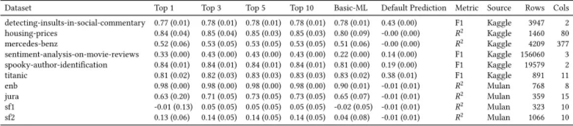
Table 4. The search space extracted from example programs, paired with a simple execution strategy, allows AL to handle a broader range of datasets.

Dataset Top 1 Top 3 Top 5 Top 10 Basic-ML Default Prediction Metric Source Rows Cols detecting-insults-in-social-commentary 0.77 (0.01) 0.78 (0.01) 0.78 (0.01) 0.78 (0.01) 0.78 (0.01) 0.43 (0.00) F1 Kaggle 3947 2 housing-prices 0.84 (0.04) 0.85 (0.04) 0.85 (0.03) 0.85 (0.03) 0.80 (0.09) -0.00 (0.00) R2 _{Kaggle 1460 80} mercedes-benz 0.52 (0.06) 0.53 (0.05) 0.53 (0.05) 0.53 (0.05) 0.51 (0.06) -0.00 (0.00) R2 _{Kaggle 4209 377} sentiment-analysis-on-movie-reviews 0.33 (0.00) 0.43 (0.00) 0.43 (0.00) 0.43 (0.00) 0.22 (0.00) 0.14 (0.00) F1 Kaggle 156060 3 spooky-author-identification 0.84 (0.01) 0.84 (0.01) 0.84 (0.01) 0.84 (0.01) 0.81 (0.00) 0.19 (0.00) F1 Kaggle 19579 2 titanic 0.81 (0.02) 0.82 (0.03) 0.83 (0.03) 0.83 (0.03) 0.83 (0.02) 0.38 (0.01) F1 Kaggle 891 11 enb 0.98 (0.00) 0.98 (0.00) 0.98 (0.00) 0.98 (0.00) 0.90 (0.01) -0.01 (0.01) R2 _{Mulan 768 8} jura 0.63 (0.20) 0.71 (0.05) 0.73 (0.05) 0.73 (0.05) 0.65 (0.07) -0.01 (0.01) R2 _{Mulan 359 15} sf1 -0.01 (0.13) 0.05 (0.05) 0.05 (0.05) 0.05 (0.05) -0.02 (0.05) -0.01 (0.01) R2 _{Mulan 323 10} sf2 0.13 (0.06) 0.14 (0.05) 0.14 (0.05) 0.14 (0.05) 0.04 (0.08) -0.01 (0.01) R2 _{Mulan 1066 10}

vector. For other systems to execute, the analyst would have to manually write code that transforms strings to numeric encodings, combines dense and spare matrix representations, and then performs any remaining necessary transformations, such as imputation. AL’s key advantage is it removes the need for this additional code.

AL handles datasets with text fields without manually adding pre-processing because the example programs used to train AL have components that process text fields automatically. Specifically, the set of transforms extracted from its training programs includes a TF-IDF transformation [Salton

and Buckley 1988] and a transform to convert strings to simple token frequency.

Both Autosklearn and TPOT fail out-of-the-box on the Mulan datasets because neither system as currently implemented handles multivariate regression [Autosklearn 2017;TPOT 2018]. An analyst intending to use these systems would have to manually piece together a separate pipeline search for each target variable, making sure that transformations in the pre-processing stage are unified across pipelines after obtaining the resulting pipelines from each tool’s search. AL executes without additional extension.

AL handles multivariate regression without manual extension because some of the example programs used to train AL have components that support multivariate regression and AL is able to construct successful pipelines using these components. By not introducing additional constraints on the search space or the characteristics of expected inputs/outputs, AL is able to produce executable pipelines for these datasets.

For 8 of these 10 datasets AL’s top 10 pipelines include a program that outperforms the Basic-ML baseline. For 2 of these 10 datasets the performance is roughly equal. Recall that the Basic-ML baseline involves manually written code to preprocess inputs and assemble the prediction pipeline. In all cases, AL outperforms the Default Prediction baseline.

Performance on two of the multi-target regression datasets (sf1 and sf2), although better than Basic-ML and Default Prediction, is still poor. We inspected the pipelines produced and found that the component choices were reasonable. For example, for sf1 the top ranked pipeline applies (from the sklearn.preprocessing package) LabelEncoder in a loop over columns to convert single string values to integers, then normalizes column values by applying MinMaxScaler, and finally fits a ridge regression. The poor performance is reflective of the inherent difficulty of the predictive task in both datasets. The target vectors consist of the counts of three different types of solar flares in a 24 hour period. Note that AL’s performance improves slightly for sf2, which has łmuch more error correction applied to it, and has consequently been treated as more reliablež [sol 2017]. 9.5 Conditional Probability Model and Search Space Impact

AL’s pipeline generation depends on the components extracted from training programs and the conditional probability model built from sequences of these components. To better understand

Table 5. Using components extracted from program traces by AL during training (AL-Random) improves average F1 scores for the top 10 pipelines relative to a random search over the entire Scikit-Learn and XGBoost libraries in 19 of the 21 datasets. Adding the conditional probability model (AL) during search produces additional improvements in 19 of the 21 OpenML and PMLB datasets.

Dataset AL AL-Random Sklearn-XGBoost-Random 1049 0.74 (0.04) 0.68 (0.13) 0.64 (0.11) 1120 0.85 (0.00) 0.82 (0.03) 0.70 (0.14) 1128 0.90 (0.12) 0.91 (0.10) 0.94 (0.02) 179 0.65 (0.18) 0.76 (0.02) 0.67 (0.13) 184 0.67 (0.06) 0.65 (0.15) 0.33 (0.23) 293 0.71 (0.28) 0.33 (0.36) 0.24 (0.39) 38 0.89 (0.03) 0.68 (0.25) 0.35 (0.37) 389 0.37 (0.17) 0.36 (0.18) 0.15 (0.21) 46 0.95 (0.01) 0.92 (0.11) 0.84 (0.18) 554 0.94 (0.03) 0.89 (0.06) 0.89 (0.05) 772 0.50 (0.03) 0.48 (0.06) 0.45 (0.09) 917 0.81 (0.06) 0.78 (0.09) 0.65 (0.15) Hill_Valley_with_noise 0.72 (0.06) 0.63 (0.15) 0.58 (0.18) Hill_Valley_without_noise 0.72 (0.10) 0.69 (0.19) 0.60 (0.23) breast-cancer-wisconsin 0.96 (0.02) 0.93 (0.10) 0.85 (0.18) car-evaluation 0.89 (0.08) 0.85 (0.11) 0.66 (0.20) glass 0.66 (0.08) 0.61 (0.12) 0.45 (0.18) ionosphere 0.92 (0.03) 0.90 (0.05) 0.84 (0.13) spambase 0.94 (0.01) 0.89 (0.15) 0.82 (0.20) wine-quality-red 0.35 (0.05) 0.33 (0.05) 0.22 (0.11) wine-quality-white 0.44 (0.05) 0.37 (0.09) 0.28 (0.13)

the impact of this conditional probability model, we compared the pipelines generated by AL on the OpenML and PMLB datasets to two alternative strategies. Sklearn-XGBoost-Random: randomly searches over all classes in Scikit-Learn and XGBoost. AL-Random: searches only over classes extracted by AL but ranks components randomly and prunes pipelines randomly.

Table5shows the average F1 score for the top 10 pipelines generated by AL-Random is higher than Sklearn-XGBoost-Random for 19 of the 21 datasets. This highlights the effectiveness of the extracted component space. AL, which uses the conditional probability model, produces further improvements in 19 of the 21 datasets over AL-Random, showing the benefits of a guiding pipeline generation through likelihood.

9.6 Search Times for Different Models

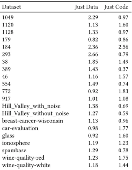
Table6shows the average search time on OpenML datasets across different model configurations relative to the search time when using the AL conditional probability model. Just Data and Just Code show the ratios when using a conditional probability model that just conditions on the data summarization features (output of α ) and the order of library classes, respectively. We found that for 17 of the 21 OpenML and PMLB datasets using the full conditional model resulted in a faster search time than just using data. However, when using just code, the benefit is less apparent, with the full conditional model providing faster search time in 11 of the 21 datasets. On average, Just Data resulted in a search time ratio of 1.38 (s.d. 0.50) and Just Code resulted in a search time ratio of 1.22 (s.d. 0.53), relative to the full conditional model.

9.7 Pipeline Distribution

Figure7summarizes the classes used in the top 1 and top 10 ranked pipelines generated by AL across benchmark datasets. Figures7aand7bshow classes that implement a learning algorithm on the x axis and the fraction of pipelines that used this component as their learning algorithm on the y axis. A taller bar indicates a more popular learning algorithm. The top ranked pipelines have a more diverse set of learning algorithms, while lower ranked pipelines tend to default to use a random forest classifier.

Table 6. Search time under different conditional probability models relative to search time under the AL model. A ratio above 1 indicates longer search time relative to AL.

Dataset Just Data Just Code

1049 2.29 0.97 1120 1.13 1.60 1128 1.33 0.97 179 0.82 0.86 184 2.36 2.56 293 2.66 0.79 38 1.85 1.49 389 1.43 0.37 46 1.16 1.57 554 1.49 0.74 772 0.92 1.83 917 1.01 1.08 Hill_Valley_with_noise 1.38 0.69 Hill_Valley_without_noise 1.27 0.59 breast-cancer-wisconsin 1.13 0.96 car-evaluation 0.98 1.77 glass 0.92 1.60 ionosphere 1.19 1.23 spambase 1.29 0.78 wine-quality-red 1.23 1.75 wine-quality-white 1.18 1.44

Figures7cand7dshows similar data for transformation classes. The generated pipelines tend to scale values before applying a learning algorithm. Lower ranked pipelines show a larger diversity of data transformations.

Approximately 8% of the top 10 pipelines generated contained 4 classes, 27% contained 3 classes, 41% contained 2 classes, and 25% contained a single class. The total number of pipelines possible, given the depth bounds, are on the order of 1e6 (of which on the order of 1e5 are executable without runtime errors). AL’s search procedure explores a fraction (on the order of 1e3) of the possible pipelines.

9.8 Comparing to Kaggle User Programs

Table7shows the performance for the top ranked pipeline produced by AL for 3 Kaggle datasets with open submissions. The first column shows the dataset. The second column shows AL’s submission score, the top user score and the percentile associated with AL’s score. AL outperformed 29%, 51% and 91% of submissions to the housing-prices, spooky-author-identification, and titanic datasets, respectively, as of this writing.

Table 7. Submissions to open Kaggle datasets. The second column should be read as AL’s score, followed by the top user scored, and the percentile associated with AL’s score. AL outperformed 29%, 51% and 91% of existing submissions as of this writing.

Dataset

AL vs Top User

Lower/Higher Better?

housing-prices 0.16 / 0.00 (29.08 percentile) Lower

spooky-author-identification 0.47 / 0.13 (51.55 percentile) Lower