Erratum: “Standing on the Shoulders of Dwarfs: The Kepler Asteroseismic LEGACY Sample. I. Oscillation Mode Parameters” (2017, ApJ, 835, 172)

HAL Id: hal-02355814

https://hal.archives-ouvertes.fr/hal-02355814

Submitted on 12 Oct 2020

HAL is a multi-disciplinary open access

archive for the deposit and dissemination of

sci-entific research documents, whether they are

pub-lished or not. The documents may come from

teaching and research institutions in France or

abroad, or from public or private research centers.

L’archive ouverte pluridisciplinaire HAL, est

destinée au dépôt et à la diffusion de documents

scientifiques de niveau recherche, publiés ou non,

émanant des établissements d’enseignement et de

recherche français ou étrangers, des laboratoires

publics ou privés.

Erratum: “Standing on the Shoulders of Dwarfs: The

Kepler Asteroseismic LEGACY Sample. I. Oscillation

Mode Parameters” (2017, ApJ, 835, 172)

Victor Silva Aguirre, Mikkel Lund, Víctor Aguirre, Guy Davies, William

Chaplin, Jørgen Christensen-Dalsgaard, Günter Houdek, Timothy White,

Timothy Bedding, Warrick Ball, et al.

To cite this version:

Victor Silva Aguirre, Mikkel Lund, Víctor Aguirre, Guy Davies, William Chaplin, et al.. Erratum:

“Standing on the Shoulders of Dwarfs: The Kepler Asteroseismic LEGACY Sample. I. Oscillation

Mode Parameters” (2017, ApJ, 835, 172). The Astrophysical Journal, American Astronomical Society,

2017, 850 (1), pp.110. �10.3847/1538-4357/aa9658�. �hal-02355814�

Erratum:

“Standing on the Shoulders of Dwarfs: The Kepler Asteroseismic LEGACY

Sample. I. Oscillation Mode Parameters

” (

2017, ApJ, 835, 172

)

Mikkel N. Lund1,2 , Víctor Silva Aguirre2 , Guy R. Davies1,2 , William J. Chaplin1,2 , Jørgen Christensen-Dalsgaard2 , Günter Houdek2 , Timothy R. White2 , Timothy R. Bedding2,3 , Warrick H. Ball4,5 , Daniel Huber2,3,6 , H. M. Antia7 ,

Yveline Lebreton8,9, David W. Latham10 , Rasmus Handberg2, Kuldeep Verma2,7 , Sarbani Basu11 , Luca Casagrande12 , Anders B. Justesen2, Hans Kjeldsen2, and Jakob R. Mosumgaard2

1_{School of Physics and Astronomy, University of Birmingham, Edgbaston, Birmingham, B15 2TT, UK;mikkelnl@phys.au.dk} 2

Stellar Astrophysics Centre, Department of Physics and Astronomy, Aarhus University, Ny Munkegade 120, DK-8000 Aarhus C, Denmark

3

Sydney Institute for Astronomy(SIfA), School of Physics, University of Sydney, NSW 2006, Australia

4

Institut für Astrophysik, Georg-August-Universität Göttingen, Friedrich-Hund-Platz 1, 37077, Göttingen, Germany

5

Max-Planck-Institut für Sonnensystemforschung, Justus-von-Liebig-Weg 3, 37077, Göttingen, Germany

6

SETI Institute, 189 Bernardo Avenue, Mountain View, CA 94043, USA

7

Tata Institute of Fundamental Research, Homi Bhabha Road, Mumbai 400005, India

8

Observatoire de Paris, GEPI, CNRS UMR 8111, F-92195 Meudon, France

9

Institut de Physique de Rennes, Université de Rennes 1, CNRS UMR 6251, F-35042 Rennes, France

10

Harvard-Smithsonian Center for Astrophysics, 60 Garden Street Cambridge, MA 02138 USA

11

Department of Astronomy, Yale University, PO Box 208101, New Haven, CT 06520-8101, USA

12_{Research School of Astronomy and Astrophysics, Mount Stromlo Observatory, The Australian National University, ACT 2611, Australia}

Received 2017 August 21; revised 2017 September 28; published 2017 November 21

Supporting material: machine-readable tables

In this erratum, we provide corrected sets of r01,10,02difference ratio values and associated uncertainties, which were overestimated in the original paper(as noted by Roxburgh2017) due to a missing trimming in the post-processing of the Markov chain Monte Carlo (MCMC) chains for these values. The typical reduction in the ratio uncertainties from performing the trimming is a factor of 10 (see Figure 3). Other parameters optimized in the peak-bagging (for instance, individual mode frequencies) are unaffected, as the trimming was performed for these in the original work (Lund et al.2017). We also provide updated values for theD2n values of l=3 modes. We note that the values presented here, as with those presented in the original work, are obtained from a single peak-bagging procedure(see Lund et al.2017for details) and have yet to be verified by independent analyses using the same input power spectra. Examples of the updated tables from the original paper are given in Tables1–3. We note that tables with individual mode parameters(Table2) have been added for completeness, but the parameters in these tables are unchanged compared to the original paper.

In addition to the corrected values mentioned above, we provide covariance matrices for the mode frequencies, frequency difference ratios(r01,10,02), and second differences ( nD2 ) for the LEGACY sample (Lund et al.2017), which were not published with the original work. The values provided by this erratum will be available in the online version of the paper.

© 2017. The American Astronomical Society. All rights reserved.

Figure 1.Comparison between ratio distribution ofr01,n=25(n »3090 Hzm ) for KIC 9139151 from the full (green) and properly thinned MCMC chains (black). The

Figure 2.Left: a comparison between ratios r01,10,02for KIC 9139151 using the full(colored) and properly thinned MCMC chains (black). The ones from the thinned

chains have been shifted 15μHz up in frequency for clarity. Middle: the ratio between the uncertainties on r01,10,02for KIC 9139151 using the original and properly

thinned MCMC chains. Right: the difference between central ratio values(given by the distribution median), asrori-rthin, for KIC 9139151. The uncertainties given

here are the reduced ones obtained using the properly thinned chains.

Figure 3.Top left: the distribution for the change in central ratio values(Dr01,10,02=rori-rnew) over the newly estimated ratio uncertainties for all LEGACY targets.

Top right: the distribution for the ratio of newly estimated ratio uncertainties from the properly thinned chains over the original estimates. Bottom left: the distribution for the ratio between ratio uncertainties calculated using properly thinned chains(sr,new) and those propagated from the frequency uncertainties (sr,freq); as expected

from Figure1, the uncertainty ratios cluster around a value of 1. Bottom right: the distribution for the ratio between the corresponding ratio values.

Corrected ratios. Concerning the updated r01,10,02values that followed the publication of the original paper, it has been suggested that the uncertainties on these were overestimated compared to expectations from the uncertainties on the individual mode frequencies(among others by Roxburgh2017). We have identified the reason for this overestimation as a missing trimming in our post-processing of the MCMC chains, which is otherwise adopted for the parameters optimized in the peak-bagging (e.g., the individual mode frequencies) and in derivingD2n values. The trimming concerns the removal of chains that for reasons unknown remain stationary during the entire MCMC run. By stationary, we mean that they did not move at all during the run (i.e., with an acceptance fraction of zero). Given that the initialization of the chains is done by sampling from the priors, the samples from these stationary chains simply represent a sparsely sampled version of the prior. Combined with the generous priors adopted for the —a 14 μHz wide top-hat prior regardless of the mode signal-to-noise ratio—these stationary chains have the

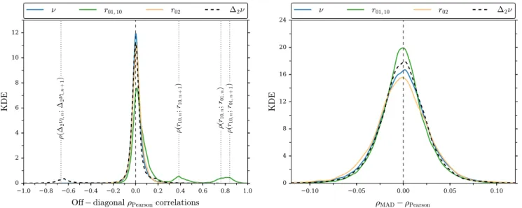
Figure 4.Left: the kernel density estimates of the off-diagonal elements of the correlation matrices for mode frequencies and frequency difference ratios(see the legend). A few of the expected correlations for r01,10ratios(dotted lines) andD2nvalues are indicated. Right: a comparison between correlations calculated using the

robust statistics method described in the original paper(r_MAD) and those estimated using the Pearson product-moment method (r_Pearson).

Figure 5.Left: the correlation matrix for the mode frequencies of 16 Cyg A(KIC 12069424). The marker sizes indicate the absolute value of the correlation (between −1 and 1), and the color indicates the sign, white (black) representing a positive (negative) value. Right: the corresponding inverse covariance matrix, including only values with∣Ci j-,1∣>1and with values above∣Ci j-,1∣=100truncated to this value.

Table 1

Extracted Mode Parameters and Quality Control for KIC 6225718(Saxo2)

n l Frequency Amplitude Line width _lnK

(μ Hz) (ppm) (μ Hz) 11 1 1351.14654-+0.697570.58628 2.2 12 0 1407.22525-+1.176190.95399 0.78512+-0.130820.08601 2.50177-+1.343402.31218 >6 12 1 1454.25081-+0.700810.53443 >6 13 0 1510.10497-+0.476740.70200 0.98745+-0.145080.10646 2.50352-+0.954262.66290 >6 13 1 1558.44725-+0.424600.54365 >6 13 2 1605.68477_-+_0.807430.74438 _1.45 14 0 1615.12079-+0.290090.24304 1.16481+-0.074840.07412 2.60127-+0.507270.67106 >6 14 1 1664.08928_-+_0.225340.20516 _>6 14 2 1711.39720-+0.595570.50377 3.14 15 0 1720.35038-+0.171920.17913 1.46219+-0.071720.06287 2.30075-+0.370500.34793 >6 15 1 1769.65111-+0.144260.14582 >6 15 2 1816.18558-+0.356360.34383 >6 16 0 1825.41345-+0.130410.12475 1.89103+-0.066050.05765 2.19171-+0.223740.33798 >6 16 1 1873.87585-+0.140810.13448 >6 16 2 1919.96748_-+_0.258880.26436 _>6 17 0 1929.04914-+0.138120.12255 2.28689+-0.060480.05624 2.84107-+0.197770.29868 >6 17 1 1977.34771_-+_0.119980.11272 _>6 17 2 2023.79957-+0.207830.21928 >6 18 0 2032.67808_-+_0.106420.11221 -+ 2.76697 0.052940.06538 2.67104-+0.182400.22980 >6 18 1 2081.57391-+0.092090.08960 >6 18 2 2128.61654-+0.157730.15407 >6 19 0 2137.58804-+0.086580.09724 3.14287+-0.061140.06464 2.49656-+0.152480.21005 >6 19 1 2186.89206-+0.089880.08049 >6 19 2 2234.70147_-+_0.158900.16414 _>6 20 0 2243.41560-+0.081410.08455 3.47475+-0.058830.06700 2.22212-+0.117380.15871 >6 19 3 2281.61498_-+_3.361301.96984 _3.01 20 1 2293.05246-+0.088440.08985 >6 20 2 2340.63219_-+_0.156870.16692 _>6 21 0 2349.63870-+0.092050.08380 3.46120+-0.061140.07072 2.61076-+0.170820.16363 >6 20 3 2385.56616-+1.155690.92790 3.94 21 1 2399.38901-+0.095180.08395 >6 21 2 2446.70610-+0.153760.15557 >6 22 0 2455.69156-+0.104610.10544 3.46269+-0.062890.07197 3.03284-+0.227680.18810 >6 21 3 2493.07764-+1.641191.24010 3.66 22 1 2505.34180_-+_0.110430.10474 _>6 22 2 2552.85151-+0.237150.22136 >6 23 0 2561.29123_-+0.140980.14766 3.17720+-0.056470.05833 4.00522-+0.181670.25373 >6 22 3 2598.55372-+1.658371.54860 3.12 23 1 2611.20028_-+0.135370.13497 >6 23 2 2658.62676-+0.319970.32668 >6 24 0 2666.48683-+0.219980.24134 2.72433+-0.044110.05767 5.23120-+0.333580.26223 >6 24 1 2717.47119-+0.171630.18160 >6 24 2 2765.04881-+0.395870.39635 >6 25 0 2773.05505_-+_0.313970.29587 -+ 2.40972 _0.056430.05210 -+ 6.75207 _0.511210.38296 _>6 25 1 2824.15430-+0.263090.26540 >6 25 2 2872.28010_-+_0.544650.54943 _>6 26 0 2879.34263-+0.503160.55896 1.95701+-0.057360.05551 7.60008-+0.814380.62881 >6 26 1 2931.24401_-+_0.340150.35125 _>6 26 2 2978.49401-+0.842890.80099 3.78 27 0 2987.14941-+0.487210.48707 1.69613-+0.061040.04189 7.53133-+0.743840.87149 >6 27 1 3038.66527-+0.526740.51048 >6 27 2 3084.55010-+1.586431.37108 1.45 28 0 3092.79984_-+_0.921020.88165 -+ 1.46461_0.060210.06604 -+ 8.85413_1.109891.43941 _>6 28 1 3145.65332-+0.620700.61323 4.92 28 2 3194.64154_-+_1.266891.68277 _2.18 29 0 3204.41215-+0.928470.88028 0.98137+-0.101040.07515 5.86594-+1.407532.75240 3.81 29 1 3251.95767-+1.470951.70914 4.2 29 2 3302.58742-+2.570392.15797 1.22 30 0 3314.17150-+2.024862.06746 1.11864+-0.079210.07356 11.64170-+1.652221.55473 3.81

Note.The complete table set(66 tables) is available in the online journal. (This table is available in its entirety in machine-readable form.)

effect of increasing the uncertainties on frequency difference ratios r01,10,02. For the updated set of derived parameters, we thus still use the MCMC chains to form distributions for the derived parameters and estimate their value from the distribution median and

Table 2

Example of Calculated Mode Frequency Difference Ratiosr01,10,02( )n (Equation (3.16) in Lund et al.2017) for KIC 6225718 (Saxo2)

Ratio type n Ratio

r02 14 0.08927-+0.007780.00748 r02 15 0.08474-+0.004840.00599 r02 16 0.08850-+0.003320.00354 r02 17 0.08777-+0.002700.00276 r02 18 0.08517-+0.002170.00230 r02 19 0.08519-+0.001650.00169 r02 20 0.08210-+0.001600.00167 r02 21 0.08468-+0.001750.00159 r02 22 0.08484-+0.001710.00173 r02 23 0.07971-+0.002410.00229 r02 24 0.07403-+0.003650.00368 r02 25 0.07500-+0.004150.00447 r02 26 0.06611-+0.006670.00658 r02 27 0.08030-+0.008400.00803 r02 28 0.07675-+0.011790.01314 r02 29 0.09203-+0.014120.01445 r10 12 0.04121-+0.009390.00961 r01 13 0.03821-+0.005450.00794 r10 13 0.03708-+0.004250.00658 r01 14 0.03647-+0.003130.00314 r10 14 0.03483-+0.002170.00225 r01 15 0.03276-+0.001810.00168 r10 15 0.03228-+0.001500.00150 r01 16 0.03325-+0.001380.00137 r10 16 0.03326-+0.001380.00134 r01 17 0.03322-+0.001280.00129 r10 17 0.03303-+0.001200.00125 r01 18 0.03239-+0.001130.00104 r10 18 0.03262-+0.000940.00101 r01 19 0.03293-+0.000940.00088 r10 19 0.03311-+0.000900.00082 r01 20 0.03288-+0.000790.00085 r10 20 0.03251-+0.000850.00087 r01 21 0.03196-+0.000860.00091 r10 21 0.03136-+0.000870.00092 r01 22 0.03086-+0.000970.00104 r10 22 0.02992-+0.001190.00118 r01 23 0.02804-+0.001500.00134 r10 23 0.02506-+0.001580.00157 r01 24 0.02190-+0.002020.00183 r10 24 0.02109-+0.002250.00220 r01 25 0.02068-+0.002740.00288 r10 25 0.01877-+0.003430.00338 r01 26 0.01709-+0.004160.00402 r10 26 0.01819-+0.003910.00419 r01 27 0.01781-+0.004860.00461 r10 27 0.01277-+0.006530.00609 r01 28 0.01303-+0.006970.00718 r10 28 0.02730-+0.006570.00658 r01 29 0.05099-+0.012140.01314

Note.The complete table set(66 tables) is available in the online journal. (This table is available in its entirety in machine-readable form.)

Table 3

Example of Calculated Second DifferencesD (2nn l, )(Equation (3.20) in Lund et al.2017) for KIC 6225718 (Saxo2)

n l D2n (μHz) 12 1 1.49165_-+1.868611.43042 13 0 1.64320-+1.652252.97338 13 1 1.19765-+1.230101.49066 14 0 0.36802-+1.089980.82532 14 1 0.13171-+0.910270.53955 14 2 -1.08414-+1.279501.54658 15 0 -0.22732_-+0.413760.51838 15 1 -1.27154-+0.452650.33595 15 2 -0.96308-+0.972060.92238 16 1 -0.76486-+0.322310.34620 16 2 0.13943-+0.780780.60583 16 0 -1.34692-+0.400270.25397 17 0 0.01785-+0.320030.27051 17 2 0.96664-+0.505510.56737 17 1 0.69395-+0.198230.37672 18 2 1.24972-+0.408560.39754 18 1 1.13328-+0.276800.20918 18 0 1.30380-+0.289420.25241 19 2 -0.15373-+0.423600.39145 19 1 0.82087-+0.189540.26296 19 0 0.88559-+0.209600.24790 20 2 0.13226-+0.372830.40859 20 3 2.59020-+2.769084.75113 20 1 0.14657-+0.182420.23765 20 0 0.42375-+0.228660.19144 21 3 -1.67592-+3.513503.17249 21 1 -0.36648-+0.240280.20448 21 2 0.15998-+0.484950.32524 21 0 -0.15729-+0.230490.21404 22 1 -0.09149-+0.271470.27138 22 2 -0.42210-+0.500120.62788 22 0 -0.44749-+0.260790.27197 23 2 0.42624-+0.531871.05611 23 0 -0.44262-+0.345380.42259 23 1 0.38138-+0.300500.37274 24 0 1.38224-+0.613810.53582 24 2 0.71863-+0.959021.08429 24 1 0.39741-+0.405930.46815 25 0 -0.20075-+0.962420.72650 25 2 -1.26870-+1.167451.55549 25 1 0.46562-+0.689340.58511 26 2 -0.14531-+1.955152.12575 26 0 1.50744-+1.263731.17357 26 1 0.35695-+0.898770.85148 27 0 -1.98217-+1.700441.10727 27 1 -0.34683-+1.343961.18152 27 2 4.79796-+4.221002.77046 28 2 -4.33698-+3.400896.79552 28 1 -0.50516-+2.177801.67785 28 0 6.76163-+2.892731.54528 29 0 -1.46290-+2.992692.11596

Note.The complete table set(66 tables) is available in the online journal. (This table is available in its entirety in machine-readable form.)

In Figure1, we give an example of the influence of the stationary chains on a specific ratio distribution for the star KIC 9139151; as seen, the ratio distribution is the result of a wide background (the ratio prior), on top of which sits the main peak from nonstationary chains.

A comparison of the newly estimated r01,10,02values and associated uncertainties to those given in the original paper are given in Figure2for the star KIC 9139151. This particular star has a substantial change in ratio uncertainties(the middle panel), while the central parameter values are insignificantly changed (the right panel). As seen, the reduction in ratio uncertainty depends on the signal-to-noise ratio of the modes involved. Comparing the r01,10,02values from the original paper to those from the properly thinned chains for all targets, we find that these have not changed significantly (see Figure3, top left). The bottom left panel of Figure3 compares the r01,10,02 uncertainties from the properly thinned chains with those obtained by sampling from the individual mode frequencies, assuming normal errors and no correlation between individual modes; the latter uncertainties thereby do not directly use the MCMC chains to calculate ratios and uncertainties, and would be the typical approach taken if only frequency values were given. From slight asymmetries that might occur in the mode frequency distributions the ratio values obtained directly from such central tendency frequency values will naturally differ to some extent from those obtained from the chains of the modes. Typically, the difference will be largest for the values that have the largest uncertainties. The bottom right panel of Figure3compares the r01,10,02 values as estimated from the properly thinned chains with those obtained by sampling from the individual mode frequencies.

UpdatedD2nl=3. In the original paper, theD2n values for l=3 modes were incorrectly estimated; in total, theD2nl=3values of 12 stars are affected by this. For convenience, we provide this erratum with the full updated lists ofD2n values for all stars.

Additional. We note that the tick labels in Figure 6 of Lund et al.(2017) are given in the incorrect order; rather than giving all r01

labels, followed by all r10 labels, these should be mixed and given as a function of increasing central radial order.

We also note that the“a” and “b” column labels in Table 4 of Lund et al. (2017) should be swapped.

Correlations and covariances. We provide the covariance matrices for the individual mode frequencies r01,10,02andD2nvalues of the sample. The original paper did not provide these, it only gave a visual representation of the r01,10,02covariance matrix for a specific star. Instead of calculating the covariance matrices using the robust statistics method described in the original paper (r_MAD), we have now opted for using the more standard Pearson product-moment correlation estimation. A reason for switching to the Pearson’s method is that the robust statistics method was found to not always result in positive-definite covariance matrices.

In the left panel of Figure4, we show the distributions for the off-diagonal elements of the correlation matrices, and also indicate a few of the expected correlations for the derived parameters. The right panel of Figure4shows the distribution for the difference in correlation value from the Pearson product-moment correlation estimation instead of the r_MADmeasure. As seen, the method adopted for estimating the correlation has an influence at the level of r = 0.05, hence correlation values with r <∣ ∣ 0.05 should be adopted cautiously. We note that the relatively large correlations between some neighboring elements of the correlation matrix, and the overall small uncertainties on the ratios, results in an inverse covariance matrix with very large values varying in sign between positive and negative—the absolute value of

c2 _{derived from comparison with another set of ratios should therefore be interpreted with care.}

In Figure 5, we provide a representation of the frequency correlation matrix (the left panel) and the corresponding inverse covariance matrix (C-1_{, the right panel) for 16 Cyg A (KIC 12069424). All points along the diagonals of theC}-1 _{matrices are} positive, and all covariance matrices(and their inverse) are positive-definite in that all eigenvalues are positive. A further check of the latter was made by testing that a Cholesky decomposition could be performed, which requires the matrix to be positive-definite. We note that the correlation matrices displayed in Roxburgh(2017), which regrettably included the stationary chains from the MCMC analysis, were shared as part of a private communication and have never been used in an analysis or appeared in the public domain. We are grateful to Ian Roxburgh for pointing out the larger than expected ratio uncertainties (Roxburgh2017), which made us aware of the missing MCMC post-processing for the estimation of frequency difference ratios. We thank the referee for comments that helped improve the erratum.

ORCID iDs Mikkel N. Lund https://orcid.org/0000-0001-9214-5642

Víctor Silva Aguirre https://orcid.org/0000-0002-6137-903X Guy R. Davies https://orcid.org/0000-0002-4290-7351 William J. Chaplin https://orcid.org/0000-0002-5714-8618 Jørgen Christensen-Dalsgaard https: //orcid.org/0000-0001-5137-0966

Günter Houdek https://orcid.org/0000-0003-1819-810X Timothy R. White https://orcid.org/0000-0002-6980-3392 Timothy R. Bedding https://orcid.org/0000-0001-5943-1460 Warrick H. Ball https://orcid.org/0000-0002-4773-1017

Daniel Huber https://orcid.org/0000-0001-8832-4488 H. M. Antia https://orcid.org/0000-0001-7549-9684 David W. Latham https://orcid.org/0000-0001-9911-7388 Kuldeep Verma https://orcid.org/0000-0003-0970-6440 Sarbani Basu https://orcid.org/0000-0002-6163-3472 Luca Casagrande https://orcid.org/0000-0003-2688-7511

References

Lund, M. N., Silva Aguirre, V., Davies, G. R., et al. 2017,ApJ,835, 172