HAL Id: hal-00295386
https://hal.archives-ouvertes.fr/hal-00295386
Submitted on 23 Jan 2004
HAL is a multi-disciplinary open access
archive for the deposit and dissemination of
sci-entific research documents, whether they are
pub-lished or not. The documents may come from
teaching and research institutions in France or
abroad, or from public or private research centers.
L’archive ouverte pluridisciplinaire HAL, est
destinée au dépôt et à la diffusion de documents
scientifiques de niveau recherche, publiés ou non,
émanant des établissements d’enseignement et de
recherche français ou étrangers, des laboratoires
publics ou privés.
comparison of nudged GCM runs with observations
M. K. van Aalst, M. M. P. van den Broek, A. Bregman, C. Brühl, B. Steil, G.
C. Toon, S. Garcelon, G. M. Hansford, R. L. Jones, T. D. Gardiner, et al.
To cite this version:
M. K. van Aalst, M. M. P. van den Broek, A. Bregman, C. Brühl, B. Steil, et al.. Trace gas transport
in the 1999/2000 Arctic winter: comparison of nudged GCM runs with observations. Atmospheric
Chemistry and Physics, European Geosciences Union, 2004, 4 (1), pp.81-93. �hal-00295386�
www.atmos-chem-phys.org/acp/4/81/
SRef-ID: 1680-7324/acp/2004-4-81
Chemistry
and Physics
Trace gas transport in the 1999/2000 Arctic winter: comparison of
nudged GCM runs with observations
M. K. van Aalst1, M. M. P. van den Broek2, A. Bregman3, C. Br ¨uhl4, B. Steil4, G. C. Toon5, S. Garcelon6, G. M. Hansford6, R. L. Jones6, T. D. Gardiner7, G. J. Roelofs1, J. Lelieveld4, and P. J. Crutzen4
1Institute for Marine and Atmospheric Research (IMAU), Utrecht, The Netherlands 2Space Research Organisation of the Netherlands (SRON), Utrecht, The Netherlands 3Royal Netherlands Meteorological Institute (KNMI), De Bilt, The Netherlands 4Max Planck Institut f¨ur Chemie (MPI), Mainz, Germany
5Jet Propulsion Laboratory (JPL), Pasadena, CA, USA 6Cambridge University, Cambridge, UK
7National Physical Laboratory (NPL), Teddington, UK
Received: 4 March 2003 – Published in Atmos. Chem. Phys. Discuss.: 15 May 2003 Revised: 13 January 2004 – Accepted: 19 January 2004 – Published: 23 January 2004
Abstract. We have compared satellite and balloon
obser-vations of methane (CH4) and hydrogen fluoride (HF) dur-ing the Arctic winter 1999/2000 with results from the MA-ECHAM4 middle atmospheric general circulation model (GCM). For this purpose, the meteorology in the model was nudged towards ECMWF analyses. This nudging technique is shown to work well for this middle atmospheric model, and offers good opportunities for the simulation of chemistry and transport processes. However, caution must be used inside the polar vortex, particularly late in the winter. The current study focuses on transport of HF and CH4, initialized with satellite measurements from the HALOE instrument aboard the UARS satellite. We have compared the model results with HALOE data and balloon measurements throughout the winter, and analyzed the uncertainties associated with tracer initialization, boundary conditions and the passive tracer as-sumption. This comparison shows that the model represents some aspects of the Arctic vortex well, including relatively small-scale features. However, while profiles outside the vor-tex match observations well, the model underestimates HF and overestimates CH4concentrations inside the vortex, par-ticularly in the middle stratosphere. This problem is also evi-dent in a comparison of vortex descent rates based upon vor-tex average tracer profiles from MA-ECHAM4, and various observations. This could be due to an underestimate of dia-batic subsidence in the model, or due to too much mixing between vortex and non-vortex air.
Correspondence to: M. K. van Aalst
1 Introduction
The Arctic winter stratosphere is one of the main areas of interest regarding the effects of increasing greenhouse gas concentrations on the middle atmosphere. The northern po-lar vortex is generally less stable and more disturbed than its southern counterpart. Consequently, the low temperatures that are necessary for the formation of polar stratospheric clouds and activation of chlorine that leads to ozone loss in spring occur less frequently, and a large-scale ozone hole is restricted to the Antarctic stratosphere. However, in the 1990s, there have been several very cold Arctic winters, in-cluding 1994–1995, 1995–1996, and 1996–1997. The 1999– 2000 winter studied here exhibited the lowest average tem-peratures on record (Manney and Sabutis, 2000), and ex-tensive denitrification and ozone destruction took place (e.g. Rex et al., 2002). At the same time, some model studies have shown that increasing greenhouse gas concentrations may in-deed cause an increase in the stability of the vortex, and a de-crease of polar middle atmospheric temperatures, resulting in enhanced ozone loss (e.g. Shindell et al., 1998, 1999; Austin et al., 2003).
To improve our understanding of these phenomena and the reliability of predictions for future ozone loss, it is crucial that climate models represent the polar vortex, and the trans-port of reactive species inside it, realistically. In particular, we want to test our middle atmospheric general circulation models (GCMs), so that they can be used, with fully coupled chemistry, to simulate the future composition and climate of the middle atmosphere. However, by their very nature, these climate models do not reproduce the weather in any particu-lar period of which we may have detailed measurements.
Hence, we can only validate their performance by assessing mean state and variability over a reasonably long time pe-riod in which sufficient observations are available. Many of the processes in climate models however, such as some of the middle atmospheric chemistry-climate interactions that are at play in polar ozone destruction, occur on much shorter time scales. Moreover, we often lack the observational record for proper validation.
To overcome some of these difficulties, we have applied, for the first time, a relaxation technique (“nudging”) to a middle-atmospheric GCM. By adding small additional ten-dencies, which hardly disturb the model’s inherent physi-cal consistency, we continuously adjust the model towards actual meteorological conditions (Jeuken et al., 1996). In this way, the model can be compared with instantaneous observations that depend on the actual meteorological situ-ation. Once tested with respect to processes on relatively short timescales, the GCM can be left free again to study longer-term changes associated with different atmospheric conditions. Such nudging techniques have been used exten-sively for tropospheric studies (e.g. de Laat et al., 1999), but not for the middle atmosphere. Until recently, the observa-tional data to be assimilated into the model, provided by the ECMWF, were only available up to 10 hPa. Since March 1999 however, a new version of the ECMWF model is oper-ational, with a new vertical resolution, and extended upwards to 0.2 hPa, equivalent to about 70 km. Using these meteoro-logical data, which are referred to as operational data (OD), we have applied this same technique in our middle atmo-spheric GCM. Once they are available, we will also be able to employ data from the ERA-40 reanalysis, which will provide data with the same model top for the entire period from 1957 to 2001 (see http://wms.ecmwf.int/research/era/index.html).
In this study, we have applied the nudging technique to test tracer transport in our MA-ECHAM4 model during the Arctic winter 1999/2000. Related transport studies with the same model include a report by Manzini and Feichter (1999), who evaluated the large-scale transport in MA-ECHAM4 by examining sulphur hexafluoride (SF6) concentrations in a 15-year integration. They showed that the model reproduced an appropriate evolution and distribution of this passive tracer, and that the mean age of air and transport barriers in the model compared favorably to observations and theory. In ad-dition, results from the MA-ECHAM4 model have been in-cluded in several stratospheric model intercomparisons, e.g. by Koshyk et al. (1999) and Pawson et al. (2000). The MA-ECHAM4 model has also been used for coupled climate-chemistry studies (Steil et al., 1998, 2003; Manzini et al., 2003), including investigations of the effect of changing at-mospheric conditions on polar dynamics and chemistry. That model version, which includes the CHEM chemical mod-ule, has also been evaluated in a model intercomparison by Austin et al. (2003).
In addition, many studies have discussed stratospheric transport of trace gases in middle atmospheric chemistry
transport models (CTMs), and show than substantial chal-lenges remain. For instance, Hall et al. (1999) showed that two- and three-dimensional chemistry transport models dif-fered markedly in their performance in relation to the age of air and the propagation of annual oscillations in tracer mix-ing ratios at the tropical tropopause (the tape recorder ef-fect). Some of these problems may be related to advection schemes, the horizontal and vertical resolution, or the mete-orological input data for the transport schemes, including the processing of those data for use in transport schemes (e.g. Bregman et al., 2003). Another possible cause for discrep-ancies, first recognized by Chipperfield et al. (1997), could be the formulation of the vertical coordinate. Recently, Ma-howald et al. (2002) presented results from IMATCH, a new version of the MATCH model that uses hybrid-isentropic co-ordinates, which are terrain following near the surface (like most models), but switch to isentropic levels from the up-per troposphere on. They show that this model version is better able to capture the observed age of air distribution and water vapor transport than the regular hybrid-pressure MATCH model, apparently due to the lower numerical verti-cal diffusion in IMATCH in the lower tropiverti-cal stratosphere region. Looking more specifically at the Arctic vortex in 1999–2000, Ray et al. (2002) showed that both descent and mixing are required to properly reproduce observed long-lived tracer-tracer correlations. Based on simple calcula-tions of changing correlacalcula-tions under different assumpcalcula-tions of the mixing processes occurring within the vortex or be-tween vortex and midlatitude air, they conclude that differ-ential descent and subsequent mixing within the vortex best reproduces the observed correlations. Plumb et al. (2002) found, based on comparisons of modeled N2O with observa-tions throughout the winter, that their model (MATCH) over-estimated N2O in the lower stratospheric vortex, due to an excess of inner-vortex mixing or an overestimate of transport across the vortex boundary. Greenblatt et al. (2002) however, found that vortex descent rates calculated by SLIMCAT and REPROBUS agreed reasonably well with observations.
To assess how our GCM is performing with respect to these transport challenges, we have compared model out-put with observations in that same Arctic winter 1999/2000, which was well studied by the Third European spheric Experiment on Ozone (THESEO) and the Strato-spheric Aerosol and Gas Experiment III (SAGE III) Ozone loss and Validation Experiment (SOLVE) campaigns. We have compared model results with satellite and balloon mea-surements of hydrogen fluoride (HF) and methane (CH4), two tracers with relatively long chemical lifetimes that can be used as passive tracers of motion, particularly in the lower stratosphere (e.g. Brasseur and Solomon, 1986). The reverse distribution of sources and sinks of HF and CH4implies that they have roughly opposite vertical profiles, HF monoton-ically increasing with altitude, and CH4 monotonically de-creasing. CH4 is emitted at the surface, and broken down mainly at higher altitudes by reaction with OH, O1D and Cl
radicals, and, above the stratopause, by photolysis. Its av-erage lifetime is more than 30 years at an altitude of 20 km, decreases to about three months at 45 km, rises again to a few years at 65 km, and then decreases to a few days above 80 km (Brasseur and Solomon, 1986). The use of HF as a tracer of stratospheric motion has been discussed extensively by Chipperfield et al. (1997). It originates in the middle and upper stratosphere as an end product of the fluorine that is re-leased in the dissociation of CFCs. Once produced, it is very inactive, with tropospheric rainout as the only significant re-moval process. Its production timescale is of the same order as the dissociation timescale of CFCs (a combination of the local photochemical destruction timescale and the overturn-ing timescale that provides “fresh” CFCs). In this study, HF and CH4were initialized with HALOE data in early Septem-ber and then advected throughout the Arctic winter. On this timescale, CH4destruction and HF production may cause the passive tracer assumption to break down, particularly in the upper stratosphere and mesosphere. Moreover, these sources and sinks may also affect concentrations lower down, par-ticularly when downward transport is relatively strong, such as in the winter polar vortex. We have tested the sensi-tivity of our results to these effects by including appropri-ate upper boundary conditions, emissions and rainout, as well as approximate 2-dimensional CH4loss rates, and com-paring these results with purely passive tracer simulations. Based upon the same initialization and constraints as pre-sented in this study, van den Broek et al. (2003), using the TM5 “zoom”-CTM, have assessed the effect of horizontal resolution on the representation of tracer transport.
Section 2 of this paper describes the measurements (satel-lite and balloon data) that we use for this comparison. Sec-tion 3 introduces our model and the nudging procedure, and Sect. 4 the experiment setup. Section 5 presents a brief overview of the conditions in the Arctic winter 1999/2000, as an introduction to Sect. 6 which presents the results of our model runs and a comparison with the data. Section 7 is a discussion of the findings, leading into the conclusion (Sect. 8).
2 Measurements
2.1 HALOE
Data from the Halogen Occultation Experiment (HALOE) were used for both the initialization of the tracer fields in our model, and for comparison with model data later in the winter. HALOE was launched on the Upper Atmosphere Re-search Satellite (UARS) spacecraft in September 1991. It is a solar occultation experiment, which uses wide band and gas cell correlation radiometry techniques in several infrared wavebands to measure vertical profiles of O3, HCl, HF, CH4, H2O, NO, NO2, aerosol extinction, and temperature versus pressure, providing a vertical resolution of about 2 km. More
details about the experiment and its instruments are provided by Russell et al. (1993). HALOE measures a set of 15 sun-set profiles and 15 sunrise profiles every day, each sun-set posi-tioned around the earth along one latitude band (one on the northern and one on the southern hemisphere). HALOE’s line of sight moves from south to north (or vice-versa) in monthly “sweeps”, providing coverage of almost the whole globe, except over the two polar caps. Given the long polar nights, HALOE coverage of the polar vortex is limited to the instances when the vortex is elongated and/or off-center, so that part of it crosses the most poleward latitudes covered by HALOE. In our Arctic winter, such observations were avail-able, among others, in early December (at about 47◦N) and late February (at about 56◦N).
In this study we have used level 2, version 19 data, avail-able at the HALOE website (http://haloedata.larc.nasa.gov). The validation of HALOE HF data is described by Russell et al. (1996). HF measurements were shown to match bal-loon observations to within 7% throughout the stratosphere above 70 mbar, at a precision smaller than 0.04 ppbv between the tropopause and the stratopause. Luo et al. (1994) gave a detailed description of the stratospheric HF distribution, based upon the new global HALOE measurements, compar-isons with previous measurements, and the NCAR 2D model. The validation of HALOE CH4 data is described by Park et al. (1996). The estimated total error in the CH4 concen-trations is about 7% between 12 and 40 km; the precision is about 0.1 ppmv at 16 km, going down to values smaller than 0.05 ppmv between 25 and 75 km. For altitudes be-low 35 km, the HALOE retrieval of chemical data uses pres-sures from NCEP assimilated meteorology. Between 35 and 85 km, pressure is retrieved from the 2.8 µm CO2band (Rus-sell et al., 1993).
2.2 Balloon data
The HALOE measurements described above have the gen-eral advantage of good spatial and temporal coverage and a large altitude range. Moreover, it is relatively straightforward to compare HALOE measurements with our model data, which result from an initialization with data of the same ori-gin. However, HALOE’s coverage is not optimal for observ-ing the polar vortex, and its vertical resolution is limited rela-tive to in-situ instruments. To circumvent these limitations, we have also included comparisons with measurements of the TDLAS and MkIV balloon-borne instruments that were deployed from Esrange (68◦N, 21◦E), near Kiruna, Sweden,
in the framework of THESEO 2000 and SOLVE.
The near-infrared Tunable Diode Laser Absorption Spec-trometer (TDLAS) from the UK National Physical Labora-tory and University of Cambridge performs in-situ measure-ments of CH4, at relatively high frequency (about every 2.3 s) and thus high vertical resolution (which of course depends upon the vertical speed of the balloon, but ranges from about 0.5 hPa in the troposphere to less than 0.1 hPa towards the
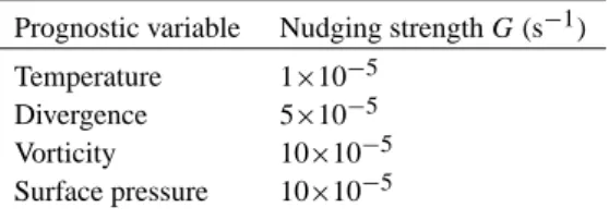
Table 1. Nudging settings, for the four nudged model variables.
Prognostic variable Nudging strength G (s−1) Temperature 1×10⁻⁵
Divergence 5×10⁻⁵ Vorticity 10×10−5 Surface pressure 10×10−5
end of the flight, between 10 and 15 hPa). The instrument is calibrated prior to flights using gas standards, with a concen-tration accuracy of 1%. The estimated absolute accuracy and the detection limit are 10% and a few ppbv, respectively. The TDLAS was deployed aboard the Systme d’Analyses par Ob-servations Z´enitales (SAOZ) platform on several days in the SOLVE/THESEO winter, including 28 January (inside the vortex; the instrument experienced a problem at the begin-ning of this flight, so data below about 78 hPa/407 K should be treated with caution), 9 February (outside the vortex), 13 February (inside the vortex, close to the edge), 27 February (inside the vortex, close to the edge) and 25 March 2000 (af-ter a vortex breakup episode, outside the vortex remnants).
The MkIV Interferometer from the Jet Propulsion Labo-ratory (JPL) is a Fourier Transform Infra-Red (FTIR) Spec-trometer (e.g. Toon, 1991). It is a remote sensing instrument, using solar occultation absorption spectroscopy in the wave-length range of 1.77 to 15.4 µm to measure a number of trace gases, including both HF and CH4, with a vertical resolu-tion of about 2 km (Toon et al., 1999). MkIV has been de-ployed on a number of aircraft and balloon missions since 1984, and has also been used extensively as a ground-based instrument. During the SOLVE/THESEO winter, MkIV was flown as part of the Observations of the Middle Stratosphere (OMS) payload on 3 December, 1999 and 15 March 2000 (both inside the vortex, at the latter date with substantial mid-latitude air mixed in at higher altitudes).
3 Model description
3.1 MA-ECHAM4
MA-ECHAM4 is the middle atmospheric version of the ECHAM4 general circulation model. It has a hybrid-pressure vertical coordinate system with 39 levels and a model top at 0.01 hPa. A description of the ECHAM4 model can be found in Roeckner et al. (1996), and details of MA-ECHAM4 are given by Manzini and McFarlane (1998) and Manzini et al. (1997). Both versions have the same basic model structure and also share most of the physical parameterizations. The main dynamical calculations are performed in spectral space, while tracer transport is calculated with a semi-Lagrangian advection scheme (Rasch and Williamson, 1990; Rasch et
al., 1995). Aside from some modifications in the radiation scheme and horizontal diffusion, MA-ECHAM4’s main dif-ference with ECHAM4 is the gravity wave parameterization. This parameterization is discussed by Manzini and lane (1998), and includes a modified version of the McFar-lane (1987) parameterization for the orographic gravity wave drag and a Doppler spread formulation of Hines (1997a, b) to parameterize the effects of the broadband gravity wave spec-trum. In this study, we have used MA-ECHAM4 at spectral triangular truncation T42, which corresponds to a horizontal resolution of about 2.8◦×2.8◦. The time step was 900 s; full radiation calculations were performed every 8 timesteps. 3.2 Nudging procedure
To ensure that the model represents actual meteorological conditions during the period under investigation, we have used a four-dimensional assimilation technique (nudging), based upon simple Newtonian relaxation. A more detailed description of this “nudging” procedure, applied in the reg-ular version of the ECHAM4 model, is given by Jeuken et al. (1996). Essentially, the model is nudged toward the ob-served state by adding a nonphysical tendency to the overall tendency of a prognostic model variable:
dX/dt =Fm(X)+G(X)×[Xobs−X]. (1) X can be any prognostic model variable (in this study we nudge surface pressure, divergence, vorticity, and tempera-ture). Fm(X) is the model forcing for variable X, G(X) the relaxation coefficient (s−1), and [Xobs−X] the
differ-ence between model and the observations. To some extent, the relaxation coefficient G can be chosen freely. However, if G is too small, the model will not be influenced by the observations. On the other hand, if G is chosen too large, the model may deviate too far from its own balanced state, leading to artificial responses to these unbalanced tenden-cies. We have adopted the optimal nudging settings from Jeuken et al. (1996) (see Table 1), who performed sensitiv-ity tests on the nudging strength of these four variables and showed that the model output depends only very weakly on the exact choice of G, particularly in the extratropics. We have checked that the nudging tendencies are generally sig-nificantly smaller than the model’s own physical tendencies, in both the lower and middle atmosphere.
The prognostic variables are relaxed toward the 6-hourly operational ECMWF data, which are produced for weather forecasting purposes. We note that we thus do not nudge towards actual observations (such as data from meteorolog-ical stations across the world, as well as satellites) but to-wards the ECMWF output, in effect an interpolation of a manifold of observations through an advanced data assimi-lation process that takes into account, for instance, the ac-curacy of the various observations. On 9 March 1999, the ECMWF deterministic forecasts switched to a 50 level model version extending to 0.2 hPa. From 12 October 1999 on, the
HF (ppb), 1 September HF (ppb), 1 December HF (ppb), 1 March CH4 (ppm), 1 September CH4 (ppm), 1 December CH4 (ppm), 1 March
0.00 0.00 1.80. 2.00. 0.23 0.45 0.68 0.90 1.13 1.35 0.58 0.25 0.50 0.75 1.00 1.25 1.50 1.75 100 200 100 200 20 10 2 1 10 20 2 1 50 50 5 5 0 0 0 0 0 0 - 90 90 - 90 90 - 90 90 - 90 90 - 90 90 - 90 90 latitude latitude latitude latitude latitude latitude pressure (hP a) pressure (hP a)
Fig. 1. Latitude versus pressure (from 200 to 1 hPa) zonal mean cross-sections of MA-ECHAM4 CH4and HF fields on 1 September (initialization), 1 December and 1 March.
vertical resolution was increased to 60 levels. To match MA-ECHAM’s vertical coordinate system and orography, a so-phisticated vertical interpolation of nudging data was per-formed by the INTERA package (Ingo Kirchner, personal communication). In this study, no nudging was applied to the top three MA-ECHAM4 levels, which lie at or above the highest ECMWF pressure level. Some caution is also required regarding the highest altitudes represented in the ECMWF model, in the upper stratosphere and lower meso-sphere. Although ECMWF analyses are readily available for these altitudes, observations to assimilate into the ECMWF model are relatively scarce. Hence, to some extent we are nudging toward the ECMWF model rather than real interpo-lated observations. Given this limitation, our analysis mainly concentrates on the lower stratosphere. Horizontally, we truncated the data from ECMWF from its original resolution of T319 to the T42 resolution of our MA-ECHAM4 runs. Fi-nally, the ECMWF data, which were available on a 6-hourly basis, were interpolated in time to match MA-ECHAM4’s time step (900 s). The spin-up time for the nudged model to reach a balanced state corresponding to a particular meteo-rological episode has been shown to be at most a few days (Jeuken et al., 1996; de Laat et al., 1999).
4 Experiment setup
The HF and CH4 tracer fields in MA-ECHAM4 were ini-tialized on 1 September, 1999, but we started our model run one month earlier to spin-up the nudging procedure, allow-ing all dynamical and physical processes, includallow-ing wave
interactions between the troposphere and the middle atmo-sphere, to reach a balanced state. The tracer initialization was based upon the zonally averaged data from the HALOE sun-set sweep of 7 August to 22 September 1999, which ranged from 73.9◦N to 63.5◦S. The HALOE data did not fill the full model domain. Vertically, we filled the top layers by extend-ing the highest HALOE data upwards, and the troposphere by prescribing tropospheric values for both species: zero for HF, 1.76 ppmv for CH4, distributed slightly over the two hemi-spheres by adding a 0.02 ppmv sine function. Between the tropospheric values and the lowest available HALOE data, we performed a straightforward log-pressure interpolation. Horizontally, we interpolated between about 43 and 62◦
lati-tude to fill a data gap in the HALOE sweep, and extrapo-lated the data from the highest available latitudes towards each pole.
These two tracer fields were then advected from 1 Septem-ber 1999 to 30 April, 2000. In the troposphere, we accounted for methane emissions by fixing the surface values, and for rainout of HF by including a two-week decay, similar to (Chipperfield et al., 1997). We simulated CH4 loss in the stratosphere and mesosphere with zonally averaged CH4loss rates from the Mainz 2D model, which includes reactions with OH, O1D and Cl as well as photolysis (Bergamaschi et al., 1996). Finally, we fixed the highest model values to the top values of the monthly zonally averaged UARS data (Ran-del et al., 1998), to account for missing chemistry and trans-port terms at the top of our model. While we included all of these processes and boundary conditions for completeness and to verify whether the passive tracer assumption would hold, sensitivity checks indicated that none of them have a
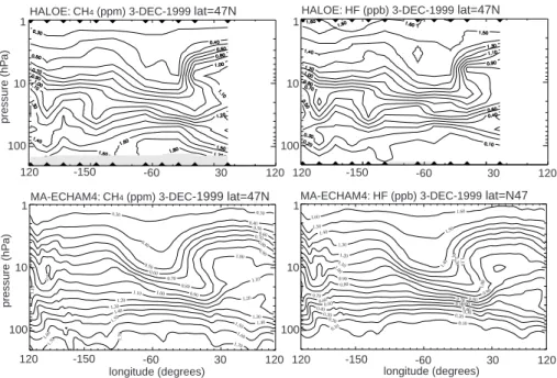
MA-ECHAM4: CH4 (ppm) 3-DEC-1999 lat=47N MA-ECHAM4: HF (ppb) 3-DEC-1999 lat=N47 HALOE: CH4 (ppm) 3-DEC-1999 lat=47N HALOE: HF (ppb) 3-DEC-1999 lat=47N 1 100 10 pressure (hP a) 1 100 10 pressure (hP a) 1 100 10 1 100 10 120 -150 -60 30 120 120 -150 -60 30 120 120 -150 -60 30 120 longitude (degrees) 120 -150 -60 30 120 longitude (degrees)
Fig. 2. Longitude versus pressure (from 200 to 1 hPa) cross-sections of HALOE observations (top) and MA-ECHAM4 fields (bottom) for
CH4(left) and HF (right) on 3 December, at 47◦latitude.
major impact on the model validation below 20 hPa, as will be shown in Fig. 8.
5 The Arctic winter 1999–2000
In 1999–2000, the vortex was already apparent in the upper and mid-stratosphere in early November. It retained a com-plex structure but became stronger and colder during Novem-ber and DecemNovem-ber, and by the end of DecemNovem-ber it also ex-tended downward into the lower stratosphere, to remain con-tinuously strong and stable during January. In February and over the course of March, upper stratospheric warmings in-fluenced the lower stratospheric circulation, and secondary cold centers developed. Nevertheless, the lower stratospheric vortex remained stable until the end of March, with cold core temperatures. Since the vortex was relatively stable through-out the winter, transport of polar air towards mid-latitudes was less intense than in many other years. However, there were several observations of polar filaments and weak trans-port, and likely stronger mixing of polar and midlatitude air during the split of the vortex related to the final warming in March. (Manney and Sabutis, 2000; European Ozone Re-search Coordinating Unit, 2000).
6 Model results
Figure 1 shows the zonally averaged CH4 and HF fields at initialization on 1 September 1999, on 1 December 1999, and on 1 March 2000. The development of the northern
win-ter vortex, indicated by a downward movement of the tracer isopleths, can be clearly identified in both HF and methane.
By comparing model data to HALOE profiles in October and November (not shown) we confirmed that the initial ini-tialization was satisfactory. On 3 December, HALOE mea-sured a longitude-altitude cross-section at about 47◦N. These
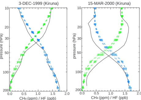
cross-sections, for CH4and HF, are compared to model data in Fig. 2. This comparison clearly shows that relatively small-scale features, including an intrusion of polar air into the midlatitudes, are well reproduced, both qualitatively and quantitatively. Nevertheless, the model does exhibit some smoothing, probably related to the numerical diffusion of the advection scheme. At that same day, MkIV balloon measure-ments were performed from Esrange, penetrating the vortex. The left frame of Fig. 3 presents a comparison of these bal-loon measurements with our model data. The fit is generally good, although there is, already this early in winter, a slight model overestimate of CH4and underestimate of HF at about 30 hPa.
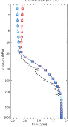
Furthermore, the model results are generally in good agreement with the profiles that were taken outside of the vortex later in the winter. For instance, the TDLAS-model comparisons in Fig. 4 show that the model fields match the CH4 measurements on 9 February very well. The same agreement was obtained for a number of high latitude HALOE profiles outside of the vortex (not shown). The agreement between the model and the measured profiles was poorer inside the vortex. For 28 January, MA-ECHAM4 overestimates CH4 relative to the TDLAS profile by 0.1– 0.3 ppmv, with the maximum displacement at 80 hPa. Simi-larly, the MkIV measurements inside the vortex on 15 March
15-MAR-2000 (Kiruna) 0.0 0.5 0.0 3-DEC-1999 (Kiruna) 0.5 2.0 2.0 1.5 1.0 1.0 1.5 50 30 20 100 100 10 10 20 30 50 200 200 CH4 (ppm) / HF (ppb) CH4 (ppm) / HF (ppb) pressure (hP a) pressure (hP a)
Fig. 3. Concentration versus pressure (from 200 to 10 hPa) plots of MA-ECHAM4 fields of HF (blue) and CH4(green) compared to MkIV observations taken from Kiruna (solid) on 3 December and 15 March. Squares represent data at model levels. Model fields were sampled at the four grid boxes surrounding the measurements.
0.0 50 30 20 100 10 200 pressure (hP a) 2.00.0 1.0 2.00.0 2.00.0 2.00.0 1.0 2.0 1.0 1.0 1.0 CH4 (ppm) CH4 (ppm) CH4 (ppm) CH4 (ppm) CH4 (ppm)
28-JAN-2000 9-FEB-2000 13-FEB-2000 27-FEB-2000 25-MAR-2000 (inside vortex) (outside vortex) (vortex edge) (vortex edge) (outside vortex)
Fig. 4. Concentration versus pressure (from 200 to 10 hPa) plots of MA-ECHAM4 CH4results (blue) compared to TDLAS observations
taken from Kiruna (solid), on 28 January (inside the vortex), 9 February (outside the vortex), 13 February (inside the vortex, close to the edge), 27 February (inside the vortex, close to the edge), and 25 March (outside the vortex). Squares represent data at model levels. Model fields were sampled at the four grid boxes surrounding the measurements.
show a model underestimate of HF everywhere in the strato-sphere up to around 12 hPa, with the largest difference of about 0.3 ppb around 25 hPa. Interestingly, there is good agreement again around 10 hPa. For CH4, there is good agreement up to about 100 hPa. At lower pressure levels, the model overestimates the concentrations (by up to 0.3 ppmv at 25 hPa). As in the case of the HF profiles, the agree-ment improves again around 10 hPa. Potential vorticity maps show that at this altitude (starting around 15 hPa), the ob-servations were no longer taken inside the vortex but at the
mixed edge or even outside it, so that we are really inter-comparing midlatitude data. The TDLAS measurements on 13 and 27 February sampled profiles inside the vortex, but close to the edge. Similar to the measurements inside the vortex, the shape of the modeled profiles is realistic, although the model tends to overestimate CH4in the stratosphere, by about 0.2 ppmv on 13 February and 0.1 ppmv on 27 Febru-ary.
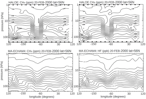
MA-ECHAM4: CH4 (ppm) 20-FEB-2000 lat=56N MA-ECHAM4: HF (ppb) 20-FEB-2000 lat=56N
HALOE: CH4 (ppm) 20-FEB-2000 lat=56N HALOE CH4 (ppm) 20-FEB-2000 lat=56N
120 -150 -60 30 120 longitude (degrees) 120 -150 -60 30 120 longitude (degrees) 120 -150 -60 30 120 120 -150 -60 30 120 1 100 10 1 100 10 1 100 10 1 100 10 pressure (hP a) pressure (hP a)
Fig. 5. Longitude versus pressure (from 200 to 1 hPa) cross-sections of HALOE observations (top) and MA-ECHAM4 fields (bottom) for
CH4(left) and HF (right) on 20 February, at 56◦latitude.
The difference between the model performance in- and outside the vortex seems to be confirmed by comparing the model results to HALOE data on 20 February. Figure 5 shows a comparison of longitude-altitude profiles at 56◦ lat-itude, cutting through the edge of the vortex at about 80◦W. At this longitude, HALOE clearly sampled vortex air (al-beit at the edge of it). Inside the vortex, a similar disagree-ment appears as in the model-balloon comparisons discussed above. For instance, at 68◦W, we obtain a good match of model and measured CH4concentrations at 100 hPa. How-ever, a difference that increases with altitude appears, up to a substantial model overestimate by about 0.6 ppmv at 20 hPa, which decreases again to a small remaining overestimate at 5 hPa. For HF, the pattern is roughly reversed, and thus con-sistent: good fit below 70 hPa, a substantial model underes-timate above this level that increases with altitude to about 0.4 ppb at 20 hPa and decreases again above 6 hPa. Outside the vortex on the other hand, the model tends to overestimate HF and underestimate CH4. While the discrepancies inside the vortex could be caused by a lack of large-scale descent, which would also be reflected at the edge of the vortex, it is also quite plausible that the model overestimates mixing be-tween vortex and midlatitude air, a phenomenon that would affect vortex edge concentrations relatively strongly. Hence, we have plotted, in Fig. 6, similar longitude-altitude profiles, but now with 3◦increments in latitude, starting at 53◦ and ending at 62◦(only HF is shown, CH4shows a similar
pat-tern). These plots clearly show that at 56◦, the model does
not yet sample “pure” vortex air, since concentration show much steeper gradients at 59◦and 62◦(all at the same longi-tude of about 80◦W). The agreement between vortex profiles from the HALOE measurements at 56◦and the model at 62◦ is much better, particularly at higher altitudes. Unfortunately, we can only speculate about what HALOE would have seen at 62◦, but these results could indicate that excessive mix-ing across the vortex edge plays a role in the discrepancies between the model and observations.
Given these anomalies, we have also assessed the model performance with respect to descent during the winter. On each first day of the month, we selected areas in the vor-tex (using the maximum PV gradients, checked by examin-ing the horizontal wind maximum) and calculated the aver-age vertical profile of the tracer concentrations versus poten-tial temperature. By tracking particular concentration lev-els as they descended to lower potential temperatures (and ascended again towards the end of the winter), we calcu-lated the descent of the air inside the vortex. These results, based on CH4profiles, are presented in Table 2 and plotted in Fig. 7. We calculated statistical errors based on the variabil-ity in the sample, and found them to be at most a few percent (note that this is the statistical error for the average profile; the variability between individual profiles is of course con-siderably larger). Very similar results were obtained when we repeated our calculations based on the HF concentrations
1 100 10 pressure (hP a) 1 100 10 pressure (hP a) 1 100 10 1 100 10 120 -150 -60 30 120 120 -150 -60 30 120 120 -150 -60 30 120 longitude (degrees) 120 -150 -60 30 120 longitude (degrees)
MA-ECHAM4: CH4 (ppm) 20-FEB-2000 lat=62N
MA-ECHAM4: CH4 (ppm) 20-FEB-2000 lat=59N
MA-ECHAM4: CH4 (ppm) 20-FEB-2000 lat=56N
MA-ECHAM4: CH4 (ppm) 20-FEB-2000 lat=53N
Fig. 6. Longitude versus pressure (from 200 to 1 hPa) cross-sections of MA-ECHAM4 HF fields on 20 February, at 53, 56, 59, and 62◦
latitude (to be compared to the HALOE observations in the top right panel of Fig. 5).
Table 2. Descent calculations, based upon MA-ECHAM results for CH4. Descent rates are given in Kelvin per day.
CH4 Initial Tpot Tpot Average Descent Descent Descent Descent
(ppmv) (1 Dec) (1 Mar) descent rate rate Dec rate Jan rate Feb rate Mar (DJF) 0.8 619 496 1.35 2.00 1.21 0.79 –0.88 1.0 557 466 0.99 1.30 1.11 0.53 –0.44 1.2 498 438 0.66 0.73 0.94 0.27 –0.26 1.4 435 409 0.28 0.36 0.62 –0.16 –0.15 1.6 370 372 –0.03 0.10 0.08 –0.29 –0.03
in our model. In Fig. 7, we compare our results to simi-lar analyses of CH4and N2O observations by Greenblatt et al. (2002). The match is quite good at higher altitudes (e.g. at early-winter potential temperatures of 500–550 K). Lower in the vortex however, the model descent rate appears to be much lower than observed, consistent with the mismatch in the earlier comparisons between observations and model out-put.
We have verified that the discrepancies cannot be caused by the lack of full chemistry, or the choice of boundary condi-tions. First of all, we note that the discrepancies do not occur outside of the vortex. Secondly, we have checked the sensi-tivity of the model concentrations to changes in the bound-ary conditions and simplified loss chemistry, and found that at the altitudes of our comparisons, there is very little
influ-ence of either the boundary conditions or the chemistry that we included in our sensitivity runs, even for the late winter. A clear example is provided in Fig. 8, where we display the same CH4balloon-model comparison of 28 January, but now with the passive tracer values (the curve that bends towards the right) and the one used above, which includes methane emissions, a top fixed to the UARS methane climatology, and 2D methane loss rates to account for reactions with Cl, O1D and OH as well as photodissociation. The calculated concentrations only start to diverge above 15 hPa. Similar graphs were obtained at other dates and places, indicating that difference between the close match of the two calcu-lated methane tracers at lower altitudes and their divergence at higher altitudes cannot be explained by a temporary and location-specific altitude-related difference in the amount of
vortex descent curves 550 400 350 450 500 -60 -40 -20 0 20 40 60
days (relative to 1-JAN-2000)
potential temper
ature (K)
black = observations red = MA-ECHAM4
Fig. 7. Vortex descent curves, showing the potential temperature
at which various fixed methane concentrations are found through the winter (horizontal: date, relative to 1 January 2000; vertical: potential temperature at which a particular concentration is found at a given date). Solid red: vortex average MA-ECHAM4. Dashed black: individual balloon measurements (Greenblatt et al., 2002). The latter were derived from individual CH4balloon observations (LACE on 19 November and 5 March, MkIV on 3 December, and BONBON on 27 January and 1 March, respectively).
mixing between inner- and outer-vortex air. Instead, it must be due to the varying influence of chemistry – negligible at lower altitudes, but more important higher up. Given that the differences are negligible below 20 hPa, uncertainties with respect to the representation of the chemistry do not affect our model-balloon comparisons.
7 Discussion
The general picture emerging from the comparison of our model results with the observations is that the model re-produces relatively small-scale features related to the polar vortex, showing that the nudging procedure enables detailed comparisons between our GCM and individual balloon or satellite measurements. Early in the winter, and later in the winter outside the vortex, the model also exhibits good quan-titative agreement with the measurements. However, there is a consistent problem later in the winter inside the vortex, where the model overestimates CH4and underestimates HF. In comparable experiments with the TM5 chemistry trans-port “zoom”-model, which was run with the same experi-mental setup and using the same ECMWF meteorology, Van den Broek et al. (2003) found very similar results. They also showed that a different initialization of the HF and CH4fields may lead to better agreement between the model and obser-vations within the vortex, but at the cost of a worse agreement at midlatitudes. Consequently, errors in the HALOE initial-ization may account for some of the offsets seen in the com-parisons, but they cannot explain the discrepancies found in the vertical gradient and over time. Hence, there are only two
0.0 0.5 1.0 1.5 2.0 CH4 (ppm) 50 500 20 100 10 200 pressure (hP a) 5 2 1 1000 28-JAN-2000 (Kiruna)
Fig. 8. Concentration versus pressure (from 200 to 10 hPa) of
MA-ECHAM4 fields of a passive CH4tracer run (red), and a similar run with methane emissions, chemistry (using 2D loss rates) and top constraints from the UARS climatology (blue), compared to TD-LAS balloon measurements (black) on 28 January 2000, inside the vortex.
main options to explain the discrepancies: a lack of descent of air from higher altitudes within the vortex, or an excess of mixing of air across the vortex edge. We note that both of these problems might cause a GCM to overestimate tempera-tures within the vortex, with potential implications for ozone chemistry.
A lack of descent of air from higher altitudes within the vortex could suggest that such descent is underestimated in the ECMWF fields that we use as input for our nudging pro-cedure. ECMWF’s temperatures in the 1999–2000 winter have been shown to be quite close to (both independent and assimilated) observations (Knudsen, 2002; Knudsen et al. 2002). However, the ECMWF may be underestimating the vertical velocity, possibly even while trying to assimilate the correct observed temperatures in a model that may not prop-erly represent all the key processes controlling those temper-atures. Then again, the vorticity and divergence should be
more robust, and these are the variables used in the nudg-ing procedure (along with the temperature and the surface pressure); MA-ECHAM4 itself calculates the vertical veloc-ity and the advection. Another possibilveloc-ity is that the nudging does create a realistic instantaneous meteorology, but also has a small but systematic effect on the descent in the vor-tex. Given that the vertical velocity is not nudged directly, we have no separate tendency for this effect. Hence, our cur-rent experiments did not allow us to test this hypothesis (the best way to test it might be to compare a climate run of sev-eral decades with and without nudging). However, we note that the experiments with the TM5 chemistry transport model showed similar problems (van den Broek et al., 2003). In that case, the advection was driven directly by the ECWMF winds, so that the nudging cannot be to blame in their results. Finally, Bregman et al. (2003) point out that errors may arise in the processing of vertical winds from spectral data for ad-vection schemes.
The second possible cause of the discrepancies is an ex-cess of mixing of air across the vortex edge, diluting the air that has descended from higher up. This option seems to be supported by the HALOE-model comparison on 20 Febru-ary. The TM5 “zoom” model was used to investigate whether such excessive mixing might be caused by the horizontal res-olution, which could be too coarse to properly represent the vortex edge (see Van den Broek et al., 2003). Those results show that at 2◦×3◦and even 1◦×1◦horizontal resolution, the descent does not improve. Some of the discrepancies might instead be related to the vertical resolution and coordinate system. In a model with isobaric coordinates, the regular “horizontal” isentropic transport in the stratosphere occurs partly across different isobaric levels. This can cause spu-rious vertical mixing between levels, particularly when the resolution is too coarse (e.g. Chipperfield et al., 1997, Ma-howald et al. 2002). This spurious vertical mixing could also affect mixing across the vortex edge, particularly when the vortex edge is not positioned exactly upright (as is of-ten the case). Finally, Steil et al. (2003) have suggested that the semi-Lagrangian advection scheme employed here also tends to lead to relatively weak downward transport inside the vortex and weak gradients across the vortex edge. In general, this advection scheme results in a relatively high numerical diffusion. In their experiments, Van den Broek et al. (2003) used a mass-flux advection scheme using first-order slopes (Russell and Lerner, 1993). While it is known that this first-order slopes scheme may also be insufficient to preserve strong gradients (Prather, 1986), the problems should decrease with a higher horizontal resolution. How-ever, their results did not improve when the horizontal reso-lution was raised, even up to 1◦by 1◦.
Future work could include longer runs to study the po-tential effects of the nudging routine on vertical transport, and tests at higher vertical resolution, or with other advec-tion schemes, such as the Spitfire advecadvec-tion scheme (Rasch and Lawrence, 1998), which is also employed by Steil et
al. (2003), or the Lin and Rood advection scheme (Lin and Rood, 1996), which will be incorporated in (MA-)ECHAM5.
8 Conclusions
We have nudged the meteorology in our MA-ECHAM4 model towards ECMWF analyses to compare model runs of HF and CH4, initialized with HALOE data, to balloon and satellite measurements in the SOLVE/THESEO winter 1999/2000. Overall, we find that the nudging procedure, which had not previously been applied in the middle atmo-sphere, is applicable and allows for a detailed comparison between model output and individual balloon and satellite measurements. It appears that the overall transport patterns around the Arctic vortex are reasonably well modeled. The model reproduces small-scale vortex features, and through-out the winter there is generally good quantitative agree-ment between the model and the observations, except late in the winter inside the vortex. This may be due to either an underestimate of subsidence in the vortex, or spurious mixing of mid-latitude air into the vortex. An underesti-mate of subsidence in the vortex could relate to the quality of the ECMWF data or the possibility of small but system-atic effects of the nudging on the vertical transport. Spurious mixing could be related to the choice of advection scheme, the current coordinate system, which applies pressure levels in the middle atmosphere, or the processing of the vertical wind field for tracer transport. In any case, these results sug-gest that care must be taken when studying sensitive chem-istry/transport processes in the Arctic vortex with GCMs like MA-ECHAM4.
Acknowledgement. We thank the UARS and HALOE teams for the
use of their data, as well as the other members of the TDLAS and MkIV teams, in particular I. H. Howieson, N. R. Swann, and P. T. Woods. We are very grateful to H. Cuijpers (CKO/KNMI) for his excellent ECHAM support, and to I. Kirchner from the Max Plank Institute for Meteorology in Hamburg, who provided the IN-TERA interpolation package and assisted in setting up the nudging procedure. Finally, we thank the Netherlands Computing Facilities (NCF) Foundation and computing center SARA for use of comput-ing resources.
References
Austin, J., Shindell, D., Beagley, S. R., et al.: Uncertainties and as-sessments of chemistry-climate models of the stratosphere, At-mos. Chem. Phys., 3, 1–27, 2003.
Beaver, G. M. and Russell III, J. M.: The Climatology of HCl and HF Observed by HALOE, Adv. Space Res., 21, 1373–1382, 1998.
Bergamaschi, P., Br¨uhl, C., Brenninkmeijer, C. A. M., Saueressig, G., Crowley, J. N., Grooss, J. U., Fischer, H., and Crutzen, P. J.: Implications of the large carbon kinetic isotope effect in the reaction of CH4+Cl for the 13C/12C ratio of stratospheric CH4, Geophys. Res. Lett., 23, 2227–2230, 1996.
Bregman, A., Segers, A., Krol, M., Meijer, E., and van Velthoven, P.: On the use of mass-conserving wind fields in chemistry-transport models, Atmos. Chem. Phys., 3, 447D457, 2003. Chipperfield, M. P., Lutman, E. R., Kettleborough, J. A., Pyle, J.
A., and Roche, A. E.: Model studies of chlorine deactivation and formation of ClONO2collar in the Arctic polar vortex, J.
Geophys. Res., 102, 1467–1478, 1997.
Chipperfield, M. P., Burton, M., Bell, W., et al.: On the use of HF as a reference for the comparison of stratospheric observations and models, J. Geophys. Res., 102, 12 901–12 919, 1997.
Considine, G., Deaver, L., Remsberg, E., and Russell III, J. M.: Analysis of Near-Global Trends and Variability in HALOE HF and HCl Data in the Middle Atmosphere, J. Geophys. Res., 104, 24 297–24 308, 1999.
Considine, G., Deaver, L., Remsberg, E., and Russell III, J. M.: HALOE Observations of a Slowdown in the Rate of Increase of HF in the Lower Mesosphere, Geophys. Res. Lett., 24, 3217– 3220, 1997.
De Laat, A. T. J., Zachariasse, M., Roelofs, G. J., van Velthoven, P., Dickerson, R. R., Rhoads, K. P., Oltmans, S. J., and Lelieveld, J.: Tropospheric O-3 distribution over the Indian Ocean during spring 1995 evaluated with a chemistry-climate model, J. Geo-phys. Res., 104, 13 881–13 893, 1999.
European Ozone Research Coordinating Unit: The Northern Hemi-sphere StratoHemi-sphere in the Winter and Spring of 1999/2000, Cambridge, 2001.
Gettelman, A., Holton, J. R., and Rosenlof, K. H.: Mass Fluxes of O3, CH4, N2O, and CF2Cl2in the Lower Stratosphere calculated from observational Data, J. Geophys. Res. 102, 19 149–19 159, 1997.
Greenblatt, J. B., Jost, H.-J., Loewenstein, M., et al.: Tracer-based determination of vortex descent in the 1999-2000 Arctic winter, J. Geophys. Res., 107, D20, 8279, doi:10.1029/2001JD000937, 2002.
Hall, T. M., Waugh, D. W. , Boering, K. A., and Plumb, R. A.: Evaluation of transport in stratospheric models, J. Geophys. Res., 104 , 18 815–18 840, 1999.
Hines, C. O.: Doppler spread parameterization of gravity wave mo-mentum deposition in the middle atmosphere. Part 1: Basic for-mulation, J. Atmos. Solar Terr. Phys., 59, 371–386, 1997a. Hines, C. O.: Doppler spread parameterization of gravity wave
mo-mentum deposition in the middle atmosphere. Part 2: Broad and quasi monochromatic spectra and implementation, J. Atmos. So-lar Terr. Phys., 59, 387–400, 1997b.
Jeuken, A. B. M., Siegmund, P. C., Heijboer, L. C., Feichter, J., and Bengtson, L.: On the potential of assimilating meteorological analysis in a climate model for the purpose of model validation, J. Geophys. Res., 101, 16 939–16 950, 1996.
Knudsen, B. M.: Updated ECMWF temperature accuracies, poster presentation at the European Ozone Symposium, Gothenburg, 7– 9 September, 2002.
Knudsen, B. M., Pommereau, J.-P., Garnier, A., Nunes-Pnharanda, M., Denis, L., Newman, P., Letrenne, G., and Durand, M.: Accuracy of analyzed stratospheric temperatures in the winter Arctic vortex from infrared Montgolfier long-duration balloon flights. 2. Results, J. Geophys. Res., 107, D20, doi:10.1029/2001JD001329, 2002.
Koshyk, J. N., Boville, B. A., Hamilton, K., Manzini, E., and Shibata, K.: Kinetic energy spectrum of horizontal motions
in middle-atmosphere models, J. Geophys. Res., 104, 27 177– 27 190, 1999.
Lin, S. J. and Rood, R.: Multi-dimensional flux-form semi-Lagrangian transport schemes, Mon. Weather Rev., 124, 2046– 2070, 1996.
Liu, X., Murcray, F. J., Murcray, D. G., and Russell III, J. M.: Comparison of HF and HCl Vertical Profiles from Ground-Based High-Resolution Infrared Solar Spectra with Halogen Occulta-tion Experiment ObservaOcculta-tions, J. Geophys. Res., 101, 10 175– 10 182, 1996.
Luo, M., Cicerone, R. J., and Russell III, J. M.: Analysis of Halo-gen Occultation Experiment HF Versus CH4Correlation Plots: Chemistry and Transport Implications, J. Geophys. Res., 100, 13 927–13 937, 1995.
Mahowald, N. M., Plumb, R. A., Rasch, P. J., del Corral, J., Sassi, F., and Heres, W.: Stratospheric transport in a 3-dimensional isentropic coordinate model, J. Geophys. Res, 107, D15, 2001JD1313, 2002.
Manney, G. L. and Sabutis, J. L.: Development of the polar vortex in the 1999–2000 Arctic winter stratosphere, Geophys. Res. Lett., 27, 2589–2592, 2000.
Manzini, E. and Feichter, J.: Simulation of the SF6 tracer with the middle atmosphere MAECHAM4 model: Aspects of the large-scale transport, J. Geophys. Res., 104, 31 097–31 108, 1999. Manzini, E. and McFarlane, N. A.: The effect of varying the source
spectrum of a gravity wave parameterization in a middle atmo-sphere general circulation model, J. Geophys. Res., 103, 31 523– 31 539, 1998.
Manzini, E., McFarlane, N. A., and McLandress, C.: Impact of the Doppler spread parameterization on the simulation of the middle atmosphere circulation using the MA/ECHAM4 general circula-tion model, J. Geophys. Res., 102, 25 751–25 762, 1997. Manzini, E., Steil, B., Br¨uhl, C., Giorgetta, M. A., and Kr¨uger, K.:
A new interactive chemistry-climate model: 2. Sensitivity of the middle atmosphere to ozone depletion and increase in green-house gases and implications for recent stratospheric cooling, J. Geophys. Res., 108, D14, 4429, doi:10.1029/2002JD002977, 2003.
McFarlane, N. A.: The effect of orographically exited gravity wave drag on the general circulation of the lower stratosphere and tro-posphere, J. Atmos. Sci., 44, 1775–1800, 1987.
M¨uller, R., Grooss, J.-U., McKenna, D. S., Crutzen, P. J., Br¨uhl, C., Russell III, J. M., and Tuck, A. F.: HALOE Observations of the Vertical Structure of Chemical Ozone Depletion in the Arctic Vortex During Winter and Early Spring 1996–1997, Geophys. Res. Lett., 24, 2717–2720, 1997.
Nedoluha, G. E., Siskind, D. E., Bacmeister, J. T., Bevilacqua, R. M., and Russell III, J. M.: Changes in Upper Stratospheric CH4
and NO2as measured by HALOE and Implications for Changes
in Transport, Geophys. Res. Lett., 25, 987–990, 1998.
Park, J. H. , Russell III, J. M., Gordley, L. L., Drayson, S. R., Chris Benner, D., McInerney, J., Gunson, M. R., Toon, G. G., Sen, B., Blavier, J.-F., Webster, C. R., Zipf, E. C., Erdman, P., Schmidt, U., and Schiller, C.: Validation of Halogen Occultation Experi-ment CH4Measurements from the UARS, J. Geophys. Res., 101,
10 183–10 203, 1996.
Pawson, S., Kodera, K., Hamilton, K., et al.: The GCM-Reality Intercomparison Project for SPARC: Scientific Issues and Initial Results, Bull. Am. Meteorol. Soc., 81, 2000.
Plumb, R. A., Heres, W., Neu, J. L., Mahowald, N., del Corral, J., Toon, G. C., Ray, E., Moore, F., and Andrews, A. E.: Global tracer modeling during SOLVE: high latitude descent and mix-ing, J. Geophys. Res., 107, 8309, doi:10.1029/2001JD001023, 2002.
Randel, W. J., Wu, F., Russell III, J. M., Roche, A., and Waters, J. W.: Seasonal Cycles and QBO Variations in Stratospheric CH4
and H2O observed in UARS HALOE Data, J. Atmos. Sci., 55,
163–185, 1998.
Rasch, P. J., Boville, B. A., and Brasseur, G. P.: A three-dimensional general circulation model with coupled chemistry for the middle atmosphere, J. Geophys. Res., 100, 9041–9071, 1995.
Rasch, P. J. and Williamson, D. L.: On shape-preserving interpola-tion and semi-Lagrangian transport, SIAM, J. Sci. Stat. Comput., 11, 656–687, 1990.
Rasch, P. J. and Lawrence, M.: Recent development in transport methods at NCAR. MPI-Report No. 265, Max-Planck-Institut f¨ur Meteorologie, FRG, 65–75, 1998.
Ray, E. A., Moore, F. L., Elkins, J. W., Hurst, D. F., Romashkin, P. A., Dutton, G. S., and Fahey, D. W.: Descent and mixing in the 1999–2000 northern polar vortex inferred from in situ tracer measurements, J. Geophys. Res., 107, D20, 2001JD000961, 2002.
Rex, M., Salawitch, R. J., Harris, N. R. P., et al.: Chemical depletion of Arctic ozone in winter 1999/2000, J. Geophys. Res., 107, D20, 8269, doi:10.1029/2001JD000620, 2002.
Roeckner, E., Arpe, K., Bengtsson, L., Christoph, M., Claussen, M., D¨umenil, L., Esch, M., Giorgetta, M., Schlese, U., and Schulzweida, U.: The atmospheric general circulation model ECHAM4: Model description and simulation of present-day cli-mate. MPI Rep. 218, Hamburg, Germany, 1996.
Russell, G. M. and Lerner, J. A.: A new finite-differencing scheme for the tracer transport equation, J. Appl. Meteorol., 20, 1483– 1498, 1993.
Russell III, J. M., Deaver, L. E., Luo, M., Cicerone, R. J., Park, J. H., Gordley, L. L., Toon, G. C., Gunson, M. R., Traub, W. A., John-son, D. G., Jucks, K. W., Zander, R., and Nolt, I.: Validation of Hydrogen Fluoride Measurements made by the HALOE Exper-iment from the UARS Platform, J. Geophys. Res., 101, 10 163– 10 174, 1996.
Russell III, J. M., Gordley, L. L., Park, J. H., Drayson, S. R., Hes-keth, D. H., Cicerone, R. J., Tuck, A. F., Frederick, J. E., Harries, J. E., and Crutzen, P. J.: The Halogen Occultation Experiment, J. Geophys. Res., 98, 10 777–10 797, 1993.
Shindell, D. T., Miller, R. L., Schmidt, G. A., and Pandolfo, L.: Simulation of recent northern winter climate trends by greenhouse-gas forcing, Nature, 399, 452–455, 1999.
Shindell, D. T., Rind, D., and Lonergan, P.: Increased polar strato-spheric ozone losses and delayed eventual recovery owing to in-creasing greenhouse-gas concentrations, Nature, 392, 589–592, 1998.
Shindell, D. T., Schmidt, G. A., Miller, R. L., and Rind, D.: Northern Hemisphere winter climate response to greenhouse gas, ozone, solar, and volcanic forcing, J. Geophys Res, 106, 7193– 7210, 2001.
Steil, B., Dameris, M., Br¨uhl, C., Crutzen, P. J., Grewe, V., Ponater, M., and Sausen, R.: Development of a chemistry module for GCMs: first results of a multi-annual integration. Ann. Geophys., 16, 205–228, 1998.
Steil, B., Br¨uhl, C., Manzini, E., Crutzen, P. J., Lelieveld, J., Rasch, P. J., Roeckner, E., and Kr¨uger, K.: A new interactive chemistry climate model. I: Present day climatology and interan-nual variability of the middle atmosphere using the model and 9 years of HALOE/UARS data, J. Geophys. Res., 108, D9, 4290, doi:10.1029/2002JD002971, 2003.
Toon, G. C.: The JPL MkIV Interferometer, Optics and Photonics News, 2, 19–21, 1991.
Toon, G. C., Blavier, J.-F., Sen, B., et al.: Comparison of MkIV bal-loon and ER-2 aircraft measurements of atmospheric trace gases, J. Geophys Res., 104, 26 779–26 790, 1999.
Van den Broek, M. M. P., van Aalst, M. K., Bregman, A., Krol, M., Lelieveld, J., Toon, G. C., Garcelon, S., Hansford, G. M., Jones, R. L., and Gardiner, T. D.: : The impact of model grid zooming on tracer transport in the 1999/2000 Arctic polar vortex, Atmos. Chem. Phys., 3, 1833–1847, 2003.