HAL Id: hal-02884321
https://hal.archives-ouvertes.fr/hal-02884321
Submitted on 17 Dec 2020
HAL is a multi-disciplinary open access
archive for the deposit and dissemination of
sci-entific research documents, whether they are
pub-lished or not. The documents may come from
teaching and research institutions in France or
abroad, or from public or private research centers.
L’archive ouverte pluridisciplinaire HAL, est
destinée au dépôt et à la diffusion de documents
scientifiques de niveau recherche, publiés ou non,
émanant des établissements d’enseignement et de
recherche français ou étrangers, des laboratoires
publics ou privés.
Col-OSSOS: Compositional Homogeneity of Three
Kuiper Belt Binaries
Michael Marsset, Wesley Fraser, Michele Bannister, Megan Schwamb,
Rosemary Pike, Susan Benecchi, J. Kavelaars, Mike Alexandersen, Ying-Tung
Chen, Brett Gladman, et al.
To cite this version:
Michael Marsset, Wesley Fraser, Michele Bannister, Megan Schwamb, Rosemary Pike, et al..
Col-OSSOS: Compositional Homogeneity of Three Kuiper Belt Binaries. The Planetary Science Journal,
IOP Science, 2020, 1 (1), pp.16. �10.3847/PSJ/ab8cc0�. �hal-02884321�
Col-OSSOS: Compositional Homogeneity of Three Kuiper Belt Binaries
Michaël Marsset1,2 , Wesley C. Fraser2 , Michele T. Bannister3 , Megan E. Schwamb2,4 , Rosemary E Pike5,6 , Susan Benecchi7 , J. J. Kavelaars8,9 , Mike Alexandersen5,6 , Ying-Tung Chen5 , Brett J. Gladman10 ,
Stephen D. J. Gwyn8 , Jean-Marc Petit11 , and Kathryn Volk12
1
Department of Earth, Atmospheric and Planetary Sciences, MIT, 77 Massachusetts Avenue, Cambridge, MA 02139, USA;michael.marsset@qub.ac.uk 2Astrophysics Research Centre, Queenʼs University Belfast, Belfast BT7 1NN, UK
3
School of Physical and Chemical Sciences—Te Kura Matū, University of Canterbury, Private Bag 4800, Christchurch 8140, New Zealand
4
Gemini Observatory, Northern Operations Center, 670 North A’ohoku Place, Hilo, HI 96720, USA
5
Institute of Astronomy and Astrophysics, Academia Sinica; 11F of AS/NTU Astronomy-Mathematics Building, No.1, Sec. 4, Roosevelt Rd Taipei 10617, Taiwan, R.O.C.
6
Harvard & Smithsonian Center for Astrophysics, 60 Garden Street, Cambridge, MA 02138, USA
7
Planetary Science Institute, 1700 East Fort Lowell, Suite 106, Tucson, AZ 85719, USA
8
NRC-Herzberg Astronomy and Astrophysics, National Research Council of Canada, 5071 West Saanich Road, Victoria, BC V9E 2E7, Canada
9
Department of Physics and Astronomy, University of Victoria, Elliott Building, 3800 Finnerty Road, Victoria, BC V8P 5C2, Canada
10
Department of Physics and Astronomy, University of British Columbia, Vancouver, BC V6T 1Z1, Canada
11
Institut UTINAM UMR6213, CNRS, Univ. Bourgogne Franche-Comté, OSU Theta F-25000 Besançon, France
12Lunar and Planetary Laboratory, The University of Arizona, 1629 East University Boulevard, Tucson, AZ 85721, USA
Received 2020 January 22; revised 2020 April 20; accepted 2020 April 22; published 2020 May 20 Abstract
The surface characterization of Trans-Neptunian binaries(TNBs) is key to understanding the properties of the disk of planetesimals from which these objects formed. In the optical wavelengths, it has been demonstrated that most equal-sized component systems share similar colors, suggesting they have a similar composition. The color homogeneity of binary pairs contrasts with the overall diversity of colors in the Kuiper Belt, which was interpreted as evidence that Trans-Neptunian objects(TNOs) formed from a locally homogeneous and globally heterogeneous protoplanetary disk. In this paradigm, binary pairs must have formed early, before the dynamically hot TNOs were scattered out from their formation location. The latter inferences, however, relied on the assumption that the matching colors of the binary components imply matching composition. Here, we test this assumption by examining the component-resolved photometry of three TNBs found in the Outer Solar System Origins Survey:
505447 (2013SQ99), 511551 (2014UD225), and 506121 (2016BP81), across the visible and J-band
near-infrared wavelength range. We report similar colors within 2σ for the binary pairs, which is suggestive of similar reflectance spectra and hence surface composition. This advocates for gravitational collapse of pebble clouds as a possible TNO formation route. However, we stress that several similarly small TNOs, including at least one binary, have been shown to exhibit substantial spectral variability in the near-infrared, implying color equality of binary pairs is likely to be violated in some cases.
Unified Astronomy Thesaurus concepts: Trans-Neptunian objects(1705);Broad band photometry (184)
1. Introduction
Since the discovery of Plutoʼs moon Charon (Christy & Harrington 1978), more than a hundred binaries have been
detected in the Kuiper Belt,13 the population of planetesimals near and beyond the orbit of Neptune. Several mechanisms have been invoked for the origin of these systems, from mutual gravitational captures (Goldreich et al. 2002; Funato et al.
2004; Schlichting & Sari 2008) to disruptions of fast rotators
(Ortiz et al. 2012) and co-formation through gravitational
collapses of pebble clouds in the primordial turbulent disk (Johansen et al. 2007; Nesvorný et al. 2010). Each formation
mechanism is expected to result in different physical properties, such as size, size ratio, orbit pole orientation, and (dis) similarity in composition, of the Trans-Neptunian binaries’
(TNBs) components. Simulations of co-formation by gravita-tional collapses currently provide the best match to the observed properties of the equal-size TNBs (Nesvorný et al.
2019; Robinson et al.2020), including their prevalence (Noll
et al. 2008; Fraser et al. 2017; although maybe not at small sizes, Hr>7.5; Pike et al. 2020), their broad inclination distribution, and their predominantly prograde orbits(Grundy et al. 2019). This scenario also explains the high fraction of
widely separated binaries in the dynamically quiescent“cold” (low inclination and eccentricity) population of the Kuiper Belt,
compared to the dynamically “hot” component where wide
binaries would have been disrupted by Neptune scattering (Parker & Kavelaars2010; Nesvorný & Vokrouhlický 2019).
In this scenario, the TNBs would share the same composition, having accreted in the same environment.
In the optical wavelengths, Benecchi et al.(2009) found that
the components of similar-sized TNBs share the same colors and interpreted this as evidence that they have similar composition. The similar colors of the pair members further contrast with the variety of colors among the overall population of Trans-Neptunian objects(TNOs; e.g., Tegler & Romanishin
1998, 2000, 2003; Tegler et al. 2003, 2008, 2016; also see
The Planetary Science Journal, 1:16 (9pp), 2020 June https://doi.org/10.3847/PSJ/ab8cc0
© 2020. The Author(s). Published by the American Astronomical Society.
Original content from this work may be used under the terms of theCreative Commons Attribution 4.0 licence. Any further distribution of this work must maintain attribution to the author(s) and the title of the work, journal citation and DOI.
13
http://www2.lowell.edu/users/grundy/tnbs/status.html 106 binary sys-tems as of 2020 April 20.
Peixinho et al. 2003, 2012, 2015; Fraser & Brown 2012; Lacerda et al.2014; Fraser et al.2015; Pike et al.2017; Wong & Brown 2017; Alvarez-Candal et al. 2019; Marsset et al.
2019; Schwamb et al. 2019; Thirouin & Sheppard 2019),
suggesting these objects formed from a locally homogeneous and globally heterogeneous protoplanetary disk. This inference, however, relies on the assumption that matching optical colors imply matching composition. However, optical colors are not sufficient to infer compositional (dis)similarities of the binary components, because different ices and chemical elements in the outer solar system share similar optical colors(e.g., Barucci et al. 2011), and many of these elements only distinctively
reveal themselves outside of optical wavelengths. Measuring composition would normally require measuring albedo and reflectance spectra of the components across the full visible and near-infrared spectral ranges. As most TNOs are too faint for spectroscopy, one must instead rely on what near-simultaneous multiband photometry reveal as a proxy.
In this short paper, we present the colors of three TNBs across the visible and J-band wavelength range and test the assumption of an identical bulk composition for the primary and secondary components of each binary pair. To do so, we reanalyze recent near-simultaneous g-, r-, z-, and J-band photometric data collected with Gemini North through the Colors of the Outer Solar System Origins Survey(Col-OSSOS; Schwamb et al. 2019), in order to search for new TNBs and
explore the spectral(dis)similarities of their components across these spectral bands.
2. Search and Characterization of Candidate Binaries 2.1. Observations
Photometric measurements presented in this paper were collected from the ground through Col-OSSOS(PI: W. Fraser) on the 8.1m Frederick C. Gillett Gemini North Telescope on Maunakea. Col-OSSOS acquires near-simultaneous g, r, and J —and, for a subsample of objects, z (Pike et al. 2017)—
photometry of a magnitude-limited subset of the OSSOS (Bannister et al.2016,2018) sample with r<23.6 (Schwamb
et al. 2019). Measurements were acquired in a rg(z)J(z)gr
sequence to monitor any light-curve effect, using the Gemini
Multi-Object Spectrograph (GMOS; Hook et al. 2004) for
measurements in the optical wavelengths and the Near
InfraRed Imager and Spectrometer (NIRI; Hodapp et al.
2003) for those in the J band. Targets were tracked sidereally,
meaning that stars appear pointlike on the images while the TNO is elongated in the direction of its projected motion on the sky. Exposures were limited to 300s in the optical and 120s in the J band in order to minimize trailing losses and to mitigate the sky background. The telescope was dithered between consecutive exposures in the samefilter to account for pixel-to-pixel sensitivity variations. Observing circumstances for our targets can be found in Pike et al.(2017) and Schwamb et al.
(2019).
2.2. Data Reduction
The data reduction and photometric extraction of the Gemini data were performed as described in Schwamb et al. (2019).
Here, we summarize the main steps. Processing of the GMOS
data was achieved with the Gemini IRAF package. We first
used the bias images acquired as part of the GMOS calibration plan to remove the bias offset from the science frames. Master
skyflats were produced from an average of the science frames with sources masked and were used to flatten these frames. Finally, the GMOS charge-coupled device (CCD) chips were mosaicked into a single extension.
For the NIRI images,flat-fielding was performed with a master flat built from the Gemini facility calibration unit flats. We produced one sky frame for each individual science image from a rolling average of the 15 temporally closest science images with sources masked, in order to account for temporal sky variation. Images acquired at similar dither positions to the image to sky-subtract were not used to compute the average sky frame. Bad pixel maps were created from the individual dark exposures, using the longest exposures toflag dead and low-sensitive pixels, and the shortest ones to identify hot pixels. These maps were then combined with the NIRI static bad pixel map provided in the Gemini IRAF package. Individual sky-subtracted images were aligned sidereally using multiple star centroids in order to create a deep stacked image of pointlike stars that can be used to compute the mean point-spread function(PSF) of the image. A second stack was produced shifting the frames at the TNOʼs on-sky velocity derived from the Minor Planet Center (MPC) Minor Planet and Comet Ephemeris Service.14 Finally, cosmic-ray rejection was performed on the stacked images using the Python implemen-tation of the L.A.Cosmic (Laplacian Cosmic Ray Identifica-tion) algorithm.15
2.3. Trailed PSF Fitting
A binary search was performed using the complete set of GMOS and NIRI images acquired for each target in the Col-OSSOS survey. We calculated and subtracted the trailed PSF (TSF) of each image with the TRIPPy software package (Fraser et al.2016). The TSF is the equivalent of the PSF for a moving
object. The details of the method used to model the TSF are provided in Fraser et al. (2016). We describe it briefly here.
First, the PSF of each GMOS image and the NIRI stack of images was measured byfitting a Moffat profile to each stellar (pointlike) source on the frame. The best-fit solution was derived byfinding the minimum χ2residual between the mean stellar profile and the modeled Moffat profile. Next, the mean Moffat profile was subtracted from each stellar source to create a mean residual image, which was then added to the mean Moffat profile. The resulting Moffat+residual profile was convolved with a line that has the length and angle that best describes the known on-image rate of motion of the TNO to produce the TSF. The TSF was thenfitted to the TNO image using the emcee Python implementation of Foreman-Mackey et al. (2013, 2019)ʼs Markov Chain Monte Carlo (MCMC)
ensemble sampler. A total of 20 walkers with three free parameters, the(x, y) positions and flux of the TNO, were used tofind the minimum χ2residual between the model and the image. Once a solution was found, uncertainties on the parameters were calculated as the 1σ deviation of the walkers across an extra 100 iteration steps. Finally, we built stacks of the residual images acquired in the samefilter for each object in our data set in order to increase the signal-to-noise ratio of the residual and to search for very faint companions.
14http://www.minorplanetcenter.net/iau/MPEph/MPEph.html
. Orbits, and thus on-sky velocities, are those published in Bannister et al.(2018). 15
http://www.astro.yale.edu/dokkum/lacosmic/
2.4. Analysis of the Residuals
Three distinct kinds of residuals are revealed by our analysis. Thefirst kind is consistent with the TNO being a single source. In that case, the residuals are indistinguishable from the background noise, i.e., the pixel values in the region of the subtracted TNO follow a Poisson distribution (Figure 1). In
the case of a double source, two categories of residuals are observed. When the binary has roughly similar-sized compo-nents, a“butterfly” pattern is revealed as a result of subtracting a single TSF from a double-peak signal. When the brightness contrast between the two components is large, the primary is
efficiently fitted and removed by the TSF, and a round,
secondary source is revealed in the residuals. Double-TSF fitting on these double sources result in residuals that are indistinguishable from the background.
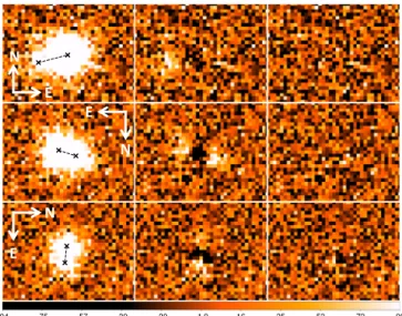
Our analysis allowed the identification of three TNBs
among 75 objects searched in the Col-OSSOS data set: 511551 (2014UD225), 506121 (2016BP81), and 505447 (2013SQ99). Images of the binaries are shown in Figure 216 and their parameters and observing circumstances are provided in Table1. All three objects come from thefirst (2014B) semester of Col-OSSOS observations and their discovery has been previously reported by Fraser et al. (2017). No other TNB
could be identified in the subsequent Col-OSSOS semesters. We attribute this to the worse seeing conditions experienced during later semesters with respect to our first semester of observations, where seeing was between 0 4 and 0 5.
In the case of 511551, the componentsʼs brightness ratio is large and single-TSF fitting efficiently removed the primary and revealed the presence of a smaller companion. In the case of 506121 and 505447, the components have roughly similar brightness, and TSF subtraction produced a“butterfly shaped” residual (Figure 2). The physical properties—angular
separa-tion and componentsʼs brightness ratio—of the three binaries are investigated in the following section.
2.5. Component-resolved Photometry
The angular separation and componentsʼs brightness ratio of the binaries were derived through double-TSF fitting using TRIPPy. We began by estimating the center position and
brightness ratio of the two binary components by eye using both the original images and the single-TSF subtracted ones. The best-fit solution was then derived for each observation through automated MCMCfitting of the sky-subtracted image. We used a total of 30 walkers, each performing a total number of a few hundred steps in the six-parameter space defined by the position and flux of the primary (x1, y1, and f1) and secondary (x2, y2, and f2) components of the binary. At each step, a standardχ2formula was used to evaluate the goodness of the fit between the synthetic double-TSF image and the science image, using an uncertainty map to mitigate the influence of bad pixels when evaluating the χ2. Once the walkers converged toward a stable solution, an additional 100 steps per walker were run and recorded. We adopted x1, y1, f1, x2, y2, and f2as best-fit parameters to the median value of these parameters across the 30×100 steps, and the uncertainty as their 1σ deviation with respect to the median value. Results of our MCMCfitting analysis for individual images are reported in Table 2. Adopted physical properties of the binaries— including their component separation and brightness ratio—are provided in Table3.
Next, we computed the component-resolved colors of the binaries by combining their measured f2/f1component bright-ness ratio with the magnitudes of the binaries converted to the Sloan Digital Sky Survey(SDSS) photometric system reported in Schwamb et al.(2019). In each image, f2/f1was calculated directly from the amplitude coefficients used to scale the TRIPPy TSFs to match image brightnesses. Fluxes were estimated from planted sources in blank images, and from both, mean colors were measured in (g − r), (r − z), and (r − J). Quoted uncertainties include the brightness ratio ranges from the fits, the Poisson statistics uncertainties, the zero-point uncertainties, the background uncertainties, and the aperture correction uncertainties. The derived (g − r), (r − z), and (r − J) colors of the binaries and their associated uncertainties Figure 1.Example of single-TSF subtraction of a non-binary TNO with the
TRIPPy software(Fraser et al. 2016). Left: original NIRI stacked image of
500836(2013 GQ137; OSSOS ID o3e21). Right: single-TSF subtracted image. The residuals are indistinguishable from the background noise. Image scales, contrast, and color bars are the same for the two images.
Figure 2.Left column: GMOS images acquired on Gemini North for 511551 (2014UD225; top), 506121 (2016BP81; middle), and 505447 (2013SQ99; bottom). Black crosses indicate the location of the two componentsʼs centroids as determined by the TSF fitting procedure. The white arrows indicate the equatorial north (N) and east (E) directions. Middle column: single-TSF subtraction reveals the binarity of the three TNOs. Right column: double-TSF subtraction efficiently removes the two binary components, with a residual consistent with the background. Image scale, contrast, and color bar are the same for all images.
16
From top to bottom, those correspond to the r-band image mrgN20140826S0221.fits of 511551 (2014UD225), the r-band image mrgN20140826S0174.fits of 506121 (2016BP81), and the g-band image mrgN20140822S0267.fits of 505447 (2013SQ99; file names listed in the Gemini Observatory Archive).
3
Table 1
Orbital Parameters and Observing Circumstances for the Three Binaries
Target MPC OSSOS a(au) e inc(°) Orbital Mean mr Hr Δ (au) rH(au) α (°) Average Mean
Number Designation ID Classification (SDSS) Air Mass MJD
511551 2014UD225 o4h45 43.36 0.130 3.66 Cold classical 22.98±0.05 6.55 43.68 44.29 1.05 1.03 56 895.554 093
” ” ” ” ” ” ” 23.17±0.04 ” 43.65 ” 1.02 1.38 56 897.438 239
506121 2016BP81 o3l39 43.68 0.076 4.18 7:4 Resonator 22.83±0.11 6.58 41.81 42.54 0.96 1.13 56 895.471 738
505447 2013SQ99 o3l76 44.15 0.093 3.47 Cold classical 23.17±0.04 6.45 46.60 47.34 0.85 1.05 56 891.544 967
Note.Geometric parameters and derived Hrare reported for the time of the Col-OSSOS observation: rH: heliocentric range,Δ: observer range, and α: phase angle. Orbital classifications are from Bannister et al. (2018). 511551(2014UD225) was observed at two distinct epochs in Col-OSSOS. Only one image from the second epoch shows evidence of binarity and was used in our analysis.
4 The Planet ary Science Journal, 1:16 (9pp ), 2020 June Marsset et al.
are reported in Table4 and are compared to the population of singletons in Figure 3.
Next, all color measurements were converted to a spectral slope (s), defined as the percentage increase in reflectance per 103Å change in wavelength normalized to 550nm, using the Synphot tool in the STSDAS software package17 (Lim et al.
2015). Specifically, this was achieved by forward modeling a
Solar spectrum convolved with a set of linear spectra, with the spectral slope varying from neutral (0%/(103Å)) to very red (50%/(103Å)) with steps of 0.1%/(103Å). We used the solar reference spectrum provided by the Hubble Space Telescope as part of the Synphot supplementary files. The array of models was then passed through Synphot to estimate the corresponding
colors in the various combinations of filters relevant for this work.
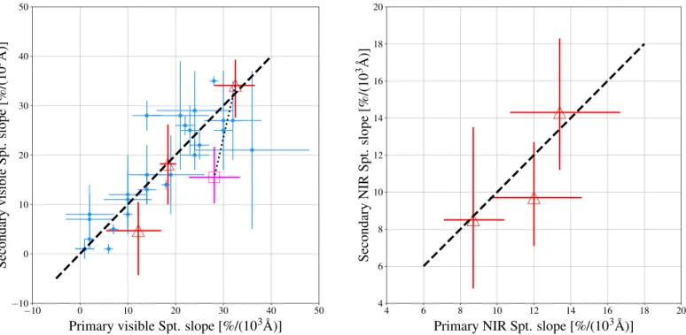
The derived spectral slope values are provided in Table5. In the left panel of Figure 4, we plot the spectral slope of the primary component versus that of the secondary in the optical wavelength range, derived from (g − r) and (r − z) colors. Spectral slope values computed from (V − I) color measure-ments in Benecchi et al. (2009) are shown for comparison
(here, the spectral slopes values were pulled directly from their paper). While these different colors do not probe the exact same wavelength range, the fact that the vast majority of TNOs exhibit linear spectral slopes in optical wavelengths makes it reasonable to compare these data sets. The right panel of Figure4shows a similar plot in the short near-infrared, derived from(r − J) color measurements. Because most TNOs show a Table 2
Results of Double-TSF Fitting
Object Image Filter MJD FWHM Separation(″) Brightness Ratiob
(″) δ R.A. cos(decl.)a δdecl.a
Distance
( )
f f 2 1 505447 N20140822S0260.fits z_G0304 56 891.505 249 5 0.42 −0.41±0.02 0.06±0.02 0.41±0.02 0.65-+0.090.13 ” N20140822S0261.fits z_G0304 56 891.509 676 1 0.33 -0.38-+0.010.02 0.04±0.02 0.38±0.01 0.54-+0.070.06 ” N20140822S0262.fits z_G0304 56 891.514 097 9 0.36 −0.37±0.01 0.02-+0.020.01 0.37-+0.020.01 0.61-+0.050.06 ” N20140822S0263.fits z_G0304 56 891.518 519 5 0.36 −0.37±0.02 0.02-+0.020.01 0.37±0.02 0.60-+0.040.05 ” N20140822S0264.fits r_G0303 56 891.522 989 9 0.39 −0.37±0.01 0.02±0.01 0.37±0.01 0.71±0.06 ” N20140822S0265.fits g_G0301 56 891.527 493 9 0.41 −0.38±0.01 0.03+-0.020.01 0.38±0.01 0.80-+0.080.06 ” N20140822S0266.fits g_G0301 56 891.531 922 0 0.41 −0.38±0.01 0.03±0.02 0.38±0.01 0.59-+0.050.06 ” N20140822S0267.fits g_G0301 56 891.536 366 1 0.45 −0.34±0.02 0.04±0.02 0.35±0.02 0.70-+0.120.10 ” O13BL3TF.fits J 56 891.586 420 4 0.44 -0.37-+0.020.03 0.02±0.02 0.38-+0.020.03 0.66-+0.060.08 511551 N20140826S0184.fits r_G0303 56 895.531 939 2 0.49 0.66-+0.040.05 0.12-+0.040.06 0.69±0.04 0.11±0.02 ” N20140826S0185.fits g_G0301 56 895.536 441 6 0.54 0.72±0.05 0.30±0.04 0.80-+0.050.04 0.12±0.02 ” N20140826S0217.fits g_G0301 56 895.600 471 2 0.53 0.65-+0.040.03 0.15+-0.040.03 0.69-+0.040.03 0.14-+0.010.02 ” N20140826S0218.fits g_G0301 56 895.604 895 8 0.52 0.67-+0.040.03 0.16±0.03 0.71-+0.040.03 0.14±0.01 ” N20140826S0219.fits g_G0301 56 895.609 328 9 0.53 0.71±0.03 0.16±0.02 0.75±0.03 0.15±0.01 ” N20140826S0220.fits r_G0303 56 895.613 824 0 0.53 0.64-+0.030.02 0.14±0.02 0.67-+0.020.03 0.14±0.01 ” N20140826S0221.fits r_G0303 56 895.618 251 1 0.53 0.58±0.02 0.16-+0.020.01 0.62±0.02 0.18±0.01 ” Col3N03.fits J 56 895.576 247 2 0.55 0.61±0.03 0.10±0.04 0.64±0.03 0.14±0.02 ” N20140828S0128.fits r_G0303 56 897.438 239 4 0.50 0.64±0.04 0.12-+0.030.02 0.65±0.04 0.14±0.02 506121 O13BL3RB.fits J 56 895.456 420 7 0.62 0.43±0.03 −0.11±0.02 0.44±0.04 0.79-+0.080.06 ” N20140826S0173.fits g_G0301 56 895.483 717 7 0.59 0.34±0.02 -0.15+-0.020.01 0.37±0.02 0.85-+0.150.09 ” N20140826S0174.fits r_G0303 56 895.487 056 2 0.50 0.36±0.01 −0.11±0.01 0.38±0.01 0.77-+0.060.07 Notes. aMeasured position of the brightest component minus position of the faintest one.
b
Measuredflux of the faintest component divided by the measured flux of the brightest one. Table 3
Mean Physical Properties of the Binaries
Object Filter Number of Separation Separation Brightness Ratio
Images (″) (103km)
( )
f f 2 1 505447 g_G0301 3 0.37-+0.010.02 12.5-+0.30.7 0.70-+0.090.08 ” r_G0303 1 0.37±0.01 12.7±0.3 0.71±0.06 ” z_G0304 4 0.38±0.02 12.9±0.7 0.60-+0.060.08 ” J 1 0.38-+0.020.03 12.9+-0.71.0 0.66-+0.060.08 511551 g_G0301 4 0.74-+0.040.03 23.5+-1.31.0 0.14-+0.010.02 ” r_G0303 4 0.66±0.03 21.0±1.0 0.14±0.01 ” J 1 0.64±0.03 20.4±0.6 0.14±0.02 506121 g_G0301 1 0.37±0.02 11.2±0.6 0.85-+0.150.09 ” r_G0303 1 0.37±0.01 11.2±0.3 0.77-+0.060.07 ” J 1 0.44±0.04 13.1±1.2 0.79-+0.080.06 17 www.stsci.edu/institute/software_hardware/stsdas 5Table 4 Colors of the Binaries
Object Color Hra (g − r) (r − z) (r − J)
Classa Binarya Primary Secondary Binarya Primary Secondary Binarya Primary Secondary
505447 red 6.45 0.98±0.03 0.97±0.07 0.99-+0.110.09 0.56±0.03 0.63±0.07 0.45±0.10 1.51±0.06 1.54-+0.090.08 1.46-+0.110.10
511551 neutral 6.55 0.74±0.02 0.74±0.03 0.74±0.13 L L L 1.42±0.06 1.42±0.06 1.42-+0.160.18
506121 neutral 6.58 0.59±0.03 0.64-+0.100.08 0.53-+0.140.09 L L L 1.60±0.07 1.59-+0.090.10 1.62-+0.100.11 Note.For comparison, solar colors are(g − r)=0.45, (r − z)=0.09, and (r − J)=0.98.
a Schwamb et al.(2019). 6 The Planet ary Science Journal, 1:16 (9pp ), 2020 June Marsset et al.
spectral inflexion close to 1 μm, these measurements are shown in a different panel from the visible data. In both wavelength ranges, none of the three binaries deviates at the >2σ level from the color correlation observed by Benecchi et al.(2009) in
the optical, implying that the binary pairs most likely share similar optical and short near-infrared colors and, therefore, similar reflectance spectra and surface composition.
The largest color difference between two binary components
in our sample is observed for 505447 (2013SQ99) and is
Δ(r − z)=0.18. 505447 is a very red object that belongs to the dynamically quiescent population of cold classical objects (Tegler & Romanishin2000; Brown2001). Compared to the g
and r photometric bands, the z band was shown to probe a distinct spectral feature that is diagnostic of cold classical surfaces(Pike et al.2017). Testing the correlation of colors in
the (r − z) wavelength range would be another useful test of surface homogeneity. Here, the observed (r − z) color differ-ence between the components of 505447 is an inconclusive 2σ result. For comparison, the largest color difference in (g − r) color is found for 506121(2016BP81), Δ(g − r)=0.11, and is contained within the 1σ error bars on the measurements.
Compared to the other two binaries in our data set, 511551 (2014UD225) exhibits a rather large brightness ratio of its components. Specifically, assuming the two components have a similar albedo, the primary would be about seven times more massive than the secondary. The similar colors of the components measured in this system suggests that the color homogeneity of TNO binaries remains valid for systems with such large mass ratios.
3. Discussion
The correlated colors of the TNB pairs across the full optical and near-infrared(J-band) spectral range advocates for similar reflectance spectra and hence surface compositions for these objects. While most TNO binaries studied so far are composed of equal mass components, this feature appears to remain valid for systems with rather large mass ratios, such as 511551 (2014UD225), where the primary is about seven times more massive than the secondary (assuming they have a similar albedo). Considering the hypothesis that TNO surfaces are primordial and indicative of their formation location(Marsset et al.2019), the surface equality of the binary pairs supports the
two key assertions made by Benecchi et al.(2009) about TNO
formation and the early outer solar system—namely, TNOs formed in a locally homogeneous and globally heterogeneous protoplanetary disk, and the formation of binaries must have happened early, before the violent dispersal of the disk that was driven by the migration of the gas giants, in order to explain the similar composition of their components. Taken together with other observed characteristics of the Kuiper Belt binaries— namely, (1) their nearly equal mass components (m2/m1> 10%; Noll et al.2008), (2) their relatively wide mutual orbits
(Parker & Kavelaars 2010), (3) their almost unanimous
prograde orbital distribution(with the exception of the widest systems; Grundy et al.2019), and (4) their predominance in the
TNO population (Fraser et al. 2017)—this finding provides
further support to the hypothesis of binary formation through the early gravitational collapse of pebble clouds in the turbulent gas disk(Nesvorný et al.2010). Only this scenario is currently
able to account simultaneously for all of the abovementioned properties of the TNO binary population. The predominance of binaries in the Kuiper Belt was recently reinforced by the New
Horizons flyby imagery of (486958)Arrokoth (2014MU69;
Stern et al.2019). This clearly showed Arrokoth to be a contact
binary, implying a high binary fraction for systems below the current telescopic limits, at least in the cold classical population.
It should be noted, however, that several small TNOs are known to exhibit substantial color variability in the near-infrared that could relate to surface inhomogeneities induced by large impacts. This is the case, for instance, for the binary 26308 Figure 3.(r − J) vs. (g − r) color–color plot of the Col-OSSOS data set from
Schwamb et al.(2019). The three binaries are marked by yellow crosses and
their individual components by blue(primary component) and cyan (secondary component) stars. The International Astronomical Union number of each binary is indicated next to the corresponding data point. Measurements of two pair members belonging to the same system are linked by a gray line. Colors of the 511551 (2014UD225) system and its components are almost equal, making them hard to distinguish in the figure. Other objects from the Col-OSSOS data set include singletons located on dynamically excited orbits(black dots) and classicals objects with i<5° (red squares). The object 2013UQ15 (magenta triangle) is bluer than the Sun in (r − J) and is dynamically consistent with the Haumea family. The solar color, with (g − r)=0.45 and (r − J)=0.98, is shown with the yellow star.
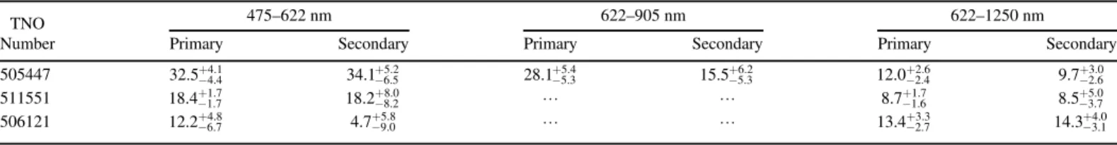
Table 5
Spectral Gradients between Two Wavelengths
TNO 475–622 nm 622–905 nm 622–1250 nm
Number Primary Secondary Primary Secondary Primary Secondary
505447 32.5-+4.44.1 34.1-+6.55.2 28.1-+5.45.3 15.5-+5.36.2 12.0-+2.42.6 9.7-+2.63.0
511551 18.4-+1.71.7 18.2-+8.28.0 L L 8.7-+1.61.7 8.5-+3.75.0
506121 12.2-+6.74.8 4.7-+9.05.8 L L 13.4-+2.73.3 14.3-+3.14.0
Note.Spectral gradients are in units of %/(103Å) and relative to 550 nm. A spectral slope of 0 corresponds to solar colors.
7
(1998SM165) that exhibits 0.2 mag variability in the J–K spectral region(Fraser et al.2015). Two non-binary TNOs in the
Col-OSSOS sample, 505448 (2013SA100) and 2013UN15,
were also found to be spectrally variable in the optical and J band (Pike et al.2017; Schwamb et al.2019). Unless both components
of such a system are rotationally locked and exhibit the same longitudinal color distributions, these highly spectrally variable systems must eventually break the color equality observed thus far. The reason why some systems were not found to have differently colored components over a large range of sizes (HV=4.0–8.1 in Benecchi et al.2009) is likely due to the low spectral variability of TNOs in the optical (Fraser et al. 2015)
with respect to the precision of the observations. It appears more likely that such a signal has merely been hidden, though we note that a few systems presented by Benecchi et al.(2009) exhibit 3σ
deviations in the color difference of the primary and secondary. Like the sample in Benecchi et al.(2009), none of the three
binaries analyzed in this work are known to be spectrally variable in the optical and near-infrared(Schwamb et al.2019).
Although photometric sequences were acquired at a single epoch for each binary, their 1.7–3.0 hr duration allowed us to investigate spectral variability but returned no hint of spectral variability. Moreover, the precision of measurements achieved in this work is insufficient to detect a 0.2 mag near-infrared color variation of the components. The required photometric precision needed to detect such variability will, however, certainly be achievable by future large ground-based facilities equipped with adaptive optics (e.g., the Extremely Large Telescope; Gilmozzi & Spyromilio 2007; the Thirty Meter Telescope; Sanders2013) and large space-based observatories
(e.g., the James-Webb Space Telescope; Gardner et al. 2006).
Future surveys of the Kuiper Belt will observe a small fraction of binary pairs with mismatched near-infrared colors.
4. Conclusion
We report component-resolved photometry for three TNBs across the visible and near-infrared spectral range. These three objects present evidence that their components have similar colors in the visible and the near-infrared, which is in agreement with Benecchi et al. (2009)ʼs finding that the
components of a given TNB always share the same optical
colors. This finding supports the inferences proposed by
Benecchi et al.(2009) that TNB pairs share the same surface
composition, thereby advocating for early binary formation in a locally homogeneous, globally heterogeneous protoplanetary disk. However, considering that several small TNBs are known to exhibit substantial color variability in the near-infrared, we anticipate that the color equality of the binary will break down in some cases as future surveys increase the known binary sample.
The authors acknowledge the sacred nature of Maunakea and appreciate the opportunity to observe from the mountain. This work is based on observations from the Large and Long
Program GN-LP-1 (2014B through 2016B), obtained at the
Gemini Observatory, which is operated by the Association of Universities for Research in Astronomy, Inc., under a cooperative agreement with the NSF on behalf of the Gemini partnership: the National Science Foundation (United States), the National Research Council (Canada), CONICYT (Chile), Ministerio de Ciencia, Tecnología e Innovación Productiva (Argentina), and Ministério da Ciência, Tecnologia e Inovação (Brazil). We thank the staff at Gemini North for their dedicated support of the Col-OSSOS program. Data was processed using the Gemini IRAF package. STSDAS and PyRAF are products of the Space Telescope Science Institute, which is operated by AURA for NASA. This research used the facilities of the Figure 4.Left: secondary vs. primary optical spectral slopes of TNBs. The blue circles correspond to previous(V − I) color measurements from Benecchi et al. (2009), and the red triangles and magenta square correspond to new measurements derived from our (g − r) and (r − z) colors, respectively. Spectral slope values for
505447(2013SQ99) derived from (g − r) and (r − z) colors are shown connected with a dotted line. Right: secondary vs. primary near-infrared (622–1250 nm) spectral slopes from this work. In both panels, the dashed line indicates a 1:1 ratio, corresponding to perfect color equality of the binary components. None of the three binaries deviate from the color correlation in the optical and short near-infrared at the 2σ level, supporting similar spectra and surface composition of their components.
Canadian Astronomy Data Centre operated by the National Research Council of Canada with the support of the Canadian Space Agency. M.M. was supported by the National Aeronautics and Space Administration under grant No. 80NSSC18K0849 issued through the Planetary Astronomy Program. B.J.G. and J.J.K. acknowledge funding from NSERC Canada. J.-M.P. acknowledges funding from PNP-INSU,
France. K.V. acknowledges funding from NASA (grants
NNX15AH59G and 80NSSC19K0785).
Facilities: Gemini:Gillett(GMOSN, NIRI), CFHT (MegaCam). Software: Astropy (Astropy Collaboration et al. 2013),
Matplotlib (Hunter2007), NumPy (van der Walt et al. 2011),
SciPy (van der Walt et al. 2011), Sextractor (Bertin &
Arnouts 1996), pyraf, TRIPPy (Fraser et al. 2016), emcee
(Foreman-Mackey et al.2013), IRAF (Tody1986), and Gemini
IRAF package, STSDAS.
ORCID iDs
Michaël Marsset https://orcid.org/0000-0001-8617-2425
Wesley C. Fraser https://orcid.org/0000-0001-6680-6558
Michele T. Bannister https: //orcid.org/0000-0003-3257-4490
Megan E. Schwamb https:
//orcid.org/0000-0003-4365-1455
Rosemary E Pike https://orcid.org/0000-0003-4797-5262
Susan Benecchi https://orcid.org/0000-0001-8821-5927
J. J. Kavelaars https://orcid.org/0000-0001-7032-5255
Mike Alexandersen https://orcid.org/0000-0003-4143-8589
Ying-Tung Chen https://orcid.org/0000-0001-7244-6069
Brett J. Gladman https://orcid.org/0000-0002-0283-2260
Stephen D. J. Gwyn https://orcid.org/0000-0001-8221-8406
Jean-Marc Petit https://orcid.org/0000-0003-0407-2266
Kathryn Volk https://orcid.org/0000-0001-8736-236X
References
Alvarez-Candal, A., Ayala-Loera, C., Gil-Hutton, R., et al. 2019, MNRAS,
488, 3035
Astropy Collaboration, Robitaille, T. P., Tollerud, E. J., et al. 2013, A&A,
558, A33
Bannister, M. T., Gladman, B. J., Kavelaars, J. J., et al. 2018,ApJS,236, 18
Bannister, M. T., Kavelaars, J. J., Petit, J.-M., et al. 2016,AJ,152, 70
Barucci, M. A., Alvarez-Candal, A., Merlin, F., et al. 2011,Icar,214, 297
Benecchi, S. D., Noll, K. S., Grundy, W. M., et al. 2009,Icar,200, 292
Bertin, E., & Arnouts, S. 1996,A&AS,117, 393
Brown, M. E. 2001,AJ,121, 2804
Christy, J. W., & Harrington, R. S. 1978,AJ,83, 1005
Foreman-Mackey, D., Farr, W., Sinha, M., et al. 2019,JOSS,4, 1864
Foreman-Mackey, D., Hogg, D. W., Lang, D., & Goodman, J. 2013,PASP,
125, 306
Fraser, W., Alexandersen, M., Schwamb, M. E., et al. 2016,AJ,151, 158
Fraser, W. C., Bannister, M. T., Pike, R. E., et al. 2017,NatAs,1, 0088
Fraser, W. C., & Brown, M. E. 2012,ApJ,749, 33
Fraser, W. C., Brown, M. E., & Glass, F. 2015,ApJ,804, 31
Funato, Y., Makino, J., Hut, P., Kokubo, E., & Kinoshita, D. 2004,Natur,
427, 518
Gardner, J. P., Mather, J. C., Clampin, M., et al. 2006,SSRv,123, 485
Gilmozzi, R., & Spyromilio, J. 2007, Msngr,127, 11
Goldreich, P., Lithwick, Y., & Sari, R. 2002,Natur,420, 643
Grundy, W. M., Noll, K. S., Roe, H. G., et al. 2019,Icar,334, 62
Hodapp, K. W., Jensen, J. B., Irwin, E. M., et al. 2003,PASP,115, 1388
Hook, I. M., Jørgensen, I., Allington-Smith, J. R., et al. 2004,PASP, 116, 425
Hunter, J. D. 2007,CSE,9, 90
Johansen, A., Oishi, J. S., Mac Low, M.-M., et al. 2007,Natur,448, 1022
Lacerda, P., Fornasier, S., Lellouch, E., et al. 2014,ApJL,793, L2
Lim, P. L., Diaz, R. I., & Laidler, V. 2015, PySynphot Userʼs Guide (Baltimore, MD: STScI),https://pysynphot.readthedocs.io/en/latest/
Marsset, M., Fraser, W. C., Pike, R. E., et al. 2019,AJ,157, 94
Nesvorný, D., Li, R., Youdin, A. N., Simon, J. B., & Grundy, W. M. 2019, NatAs,3, 808
Nesvorný, D., & Vokrouhlický, D. 2019,Icar,331, 49
Nesvorný, D., Youdin, A. N., & Richardson, D. C. 2010,AJ,140, 785
Noll, K. S., Grundy, W. M., Stephens, D. C., Levison, H. F., & Kern, S. D. 2008,Icar,194, 758
Ortiz, J. L., Thirouin, A., Campo Bagatin, A., et al. 2012,MNRAS,419, 2315
Parker, A. H., & Kavelaars, J. J. 2010,ApJL,722, L204
Peixinho, N., Delsanti, A., & Doressoundiram, A. 2015,A&A,577, A35
Peixinho, N., Delsanti, A., Guilbert-Lepoutre, A., Gafeira, R., & Lacerda, P. 2012,A&A,546, A86
Peixinho, N., Doressoundiram, A., Delsanti, A., et al. 2003,A&A,410, L29
Pike, R. E., Fraser, W. C., Schwamb, M. E., et al. 2017,AJ,154, 101
Pike, R. E., Kanwar, J., Alexandersen, M., Chen, Y.-T., & Schwamb, M. E. 2020, arXiv:2001.10144
Robinson, J. E., Fraser, W. C., Fitzsimmons, A., & Lacerda, P. 2020, A&A, submitted
Sanders, G. H. 2013,JApA,34, 81
Schlichting, H. E., & Sari, R. 2008,ApJ,673, 1218
Schwamb, M. E., Fraser, W. C., Bannister, M. T., et al. 2019, ApJS, 243, 12
Stern, S. A., Weaver, H. A., Spencer, J. R., et al. 2019,Sci,364, aaw9771
Tegler, S. C., Bauer, J. M., Romanishin, W., & Peixinho, N. 2008, in The Solar System Beyond Neptune, ed. M. A. Barucci et al.(Tucson, AZ: Univ. Arizona Press),105
Tegler, S. C., & Romanishin, W. 1998,Natur,392, 49
Tegler, S. C., & Romanishin, W. 2000,Natur,407, 979
Tegler, S. C., & Romanishin, W. 2003,Icar,161, 181
Tegler, S. C., Romanishin, W., & Consolmagno, G. J. 2003,ApJL,599, L49
Tegler, S. C., Romanishin, W., & Consolmagno, G. J. 2016,AJ,152, 210
Thirouin, A., & Sheppard, S. S. 2019,AJ,158, 53
Tody, D. 1986,Proc. SPIE,627, 733
van der Walt, S., Colbert, S. C., & Varoquaux, G. 2011,CSE,13, 22
Wong, I., & Brown, M. E. 2017,AJ,153, 145
9