A simple and fast phase transition relaxation solver for compressible multicomponent two-phase flows

Observed vs Controlled Order Parameters The competence and coverage maps (Figs. 1, 3) sug- gest that C4.5 error might be related to the coverage P c of the underlying target

3.3 Enhancing the Relaxation Riemann Solver by Sub-Iteration Algorithm 2.1 requires values for traces at phase boundaries as they appear in solutions of Riemann problems.. In

Consistent mass and momentum transport for simulating incompressible interfacial flows with large density ratios using the level set method. Contribution à l’étude des

27 (2005), 914–936], we propose a relaxation scheme for the numerical simulation of one-dimensional two-phase multi-component flows governed by a drift-flux model, the main features

We show first that the second sound overdamping leads to much longer relaxation times, as observed by ultrasonic measurements.. We show then that the technique used

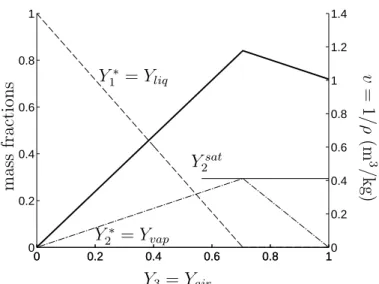
In this paragraph, we present a classical model to describe the thermodynamics behavior of mixtures. With this model, it is possible to predict some characteristics of

2014 A model based on second rank tensor orientational properties of smectic phases is developed.. The model predicts a second order smectic A-smectic C phase transition

Essentially, four flux domains are observed: the first connecting the northernmost part of the positive polarity (i.e., P0) to the negative flux N3 at its south (green field lines