HAL Id: hal-00139607
https://hal.archives-ouvertes.fr/hal-00139607
Submitted on 3 Apr 2007
HAL is a multi-disciplinary open access
archive for the deposit and dissemination of
sci-entific research documents, whether they are
pub-lished or not. The documents may come from
teaching and research institutions in France or
abroad, or from public or private research centers.
L’archive ouverte pluridisciplinaire HAL, est
destinée au dépôt et à la diffusion de documents
scientifiques de niveau recherche, publiés ou non,
émanant des établissements d’enseignement et de
recherche français ou étrangers, des laboratoires
publics ou privés.
Philippe Helluy, Nicolas Seguin
To cite this version:
Philippe Helluy, Nicolas Seguin. Relaxation models of phase transition flows. ESAIM: Mathematical
Modelling and Numerical Analysis, EDP Sciences, 2006, 40 (2), pp.331-352. �hal-00139607�
Mod´elisation Math´ematique et Analyse Num´erique
RELAXATION MODELS OF PHASE TRANSITION FLOWS
Philippe HELLUY
1and Nicolas SEGUIN
2Abstract. In this work, we propose a general framework for the construction of pressure law for
phase transition. These equations of state are particularly suitable for a use in a relaxation finite volume scheme. The approach is based on a constrained convex optimization problem on the mixture entropy. It is valid for both miscible and immiscible mixtures. We also propose a rough pressure law for modelling a super-critical fluid.
R´esum´e. Dans ce travail, on propose un cadre g´en´eral pour construire des lois de pression pour
les fluides subissant des transitions de phase. Ces lois de pression sont particuli`erement adapt´ees aux sch´emas num´eriques de relaxation. L’approche est bas´ee sur la r´esolution d’un probl`eme d’optimisation convexe avec contraintes sur l’entropie du m´elange. Les m´elanges miscibles ou immiscibles peuvent ˆetre trait´es par cette approche. Nous proposons enfin un mod`ele tr`es simple de fluide super-critique.
1991 Mathematics Subject Classification. 76M12, 65M12.
december 2005.
Introduction
The Euler equations of compressible inviscid flows possess strong non-linearities that lead to the possibility of several discontinuous solutions. It is then necessary to take into account a dissipative mechanism to select a unique solution. The most classical selection criterion is the Lax entropy criterion [21] that expresses, in a weak sense, the growth of the physical entropy. In order to converge towards the entropy solution, numerical methods have also to take into account a discrete version of the entropy criterion. Among the huge quantities of methods that have been proposed to approximate the Euler system, the relaxation approach has proved to be very interesting both on the theoretical and the practical sides [6], [29], [11], [30], [23], [10], [1], [13], [5], [2], [9] etc. The principle is to consider an augmented system, with more unknowns, that is in some sense “more linear” than the original Euler system. Then, appropriate source terms depending on a relaxation parameter λ are added to the augmented system. These source terms have two main features:
• when the parameter λ → ∞, the augmented system tends, at least formally, towards the Euler system; • they are compatible with the growth of the entropy.
Practically, a relaxation model leads to a very natural splitting method to approximate the Euler system. Each time step of the method is made of two stages. In the first stage, the augmented system is numerically solved without the source term. This resolution is simpler than for the Euler system. In the second stage, the source terms are applied.
Keywords and phrases: finite volume, entropy optimization, relaxation, phase transition, reactive flows, critical point. 1 ISITV/MNC, BP 56, 83162 La Valette cedex, France
2 Laboratoire J.-L. Lions, Universit´e Paris VI, France
c
In this paper, we concentrate on a compressible flow with phase transition. For simplicity, but without a loss of generality, we restrict to one-dimensional problems. The considered relaxation model is the following
ρt+ (ρu)x= 0,
(ρu)t+ (ρu2+ p)x= 0,
(ρε + ρu2/2)t+ ((ρε + ρu2/2 + p)u)x= 0,
Yt+ uYx= −λ(Y − Yeq).
(1)
The unknowns are the density ρ > 0, the velocity u, the internal energy ε > 0 and the vector of fractions
Y ∈ [0, 1]3, all depending on the space variable x and the time variable t. The vector of fractions is of the form
Y = (ϕ, α, z)T, where ϕ is the vapor mass fraction, α is the vapor volume fraction and z is the vapor energy
fraction. The pressure p is a function of the specific volume τ = 1/ρ, the internal energy ε and the vector of fractions Y . It is defined via the specific entropy function s : (τ, ε, Y ) → s(τ, ε, Y ). The specific entropy satisfies:
For all Y, (τ, ε) → s(τ, ε, Y ) is strictly concave;
For all (τ, ε), Y → s(τ, ε, Y ) is strictly concave;
For all (τ, ε, Y ), sε(τ, ε, Y ) > 0.
(2) It also gives the form of the pressure law
p := ∂s/∂τ
∂s/∂ε. (3)
The relaxation parameter λ is > 0. More generally, one can also consider that λ is a symmetric ≥ 0 matrix.
The equilibrium vector of fractions Yeq is defined by
s(τ, ε, Yeq(τ, ε)) = max
06Y 61s(τ, ε, Y ). (4)
With the previous conditions and definitions, the relaxation model (1) appears to be hyperbolic. The quantity U = −ρs is a Lax entropy of (1) associated to the entropy flux G = −ρus. The positivity of λ and the concavity of s with respect to Y implies that regular solutions of the system satisfies the second principle of thermodynamics
st+ usx≥ 0. (5)
In a previous paper [2], we have proposed possible forms for the entropy s(τ, ε, Y ). We have presented some numerical experiments and physical applications of the model (1). In the present work we concentrate on a procedure, inspired from the thermodynamics of mixtures, in order to design physically and mathematically coherent specific entropies s(τ, ε, Y ).
Remark 1. For a general theory of relaxation models we refer to [5]. Our relaxation system is not an entropy
extension of the relaxed system in the sense of [11] because the entropy s is generally not concave with respect to all the variables (τ, ε, Y ) (see conditions (2)). But it seems to comply with the reduced stability condition of [5]. The subcharacteristic property and the dissipativity of the leading term in the Chapman-Enskog expansion with respect to 1/λ are thus assured.
The plan of this work is the following.
In Section 1 we first recall the thermodynamics theory for a single fluid. In the classical presentations of thermodynamics (as in [20], [8], [14], [28], [12]) the starting point is the entropy function of the fluid. The pressure and temperature laws are computed from the entropy.
In Section 2 we start to state a mathematical framework for the thermodynamics of mixtures. When two different fluids are mixed and if the entropies are known, it is possible to find the mixture entropy after the resolution of a convex optimization problem. The pressure law resulting from this computation is the well-known
isobaric law: at equilibrium, the pressure law is the common pressure of the two phases. It also appears that the mixture entropy is the sup-convolution of the entropies of the two phases. This fact is not difficult to notice but we have not found it in the classical literature. We then give a simple illustration of the previous theory. We compute the equilibrium of two phases satisfying the perfect gas law.
In Section 3, thanks to several numerical experiments, we will see that it is possible, in some cases, to capture several solutions satisfying an increasing entropy principle. This phenomenon is studied by St´ephane Jaouen in his thesis [19].
In Section 4 we show that the previous theory can also be applied to miscible mixtures. It can be done by only changing the constraints in the optimization problem. The resulting pressure law is then the Dalton law: the pressure of the mixture is the sum of the partial pressures of the two phases. We give a simple example. We also propose a tentative modelling of the critical behavior. The idea is to modify the constraints in such a way that the mixture becomes more and more “miscible” when the energy increases. With this very rough approach, we are able to recover some features of a critical behavior: bounded saturation line, saturation region ending up at a critical temperature.
1.
Thermodynamics of a single fluid
1.1. Entropy
Consider a single fluid of mass M ≥ 0, internal energy E ≥ 0, occupying a volume V ≥ 0. If the fluid is homogeneous and at rest, its behavior is entirely defined by its entropy function
S : (M, V, E) → S(M, V, E). (6)
In the sequel, we note W = (M, V, E). The vector W belongs to a closed convex cone of R3, C = {(M, V, E),
M ≥ 0, V ≥ 0, E ≥ 0}. According to thermodynamics the entropy function must satisfy • The entropy S is positively homogeneous of degree 1 (in short: “S is PH1”)
∀λ > 0, S(λW ) = λS(W ). (7)
• The entropy S(W ) is concave with respect to W .
The chosen axiomatic is justified in [8], [14]. In the sequel, we will sometimes suppose more regularity of W → S(W ) (as the existence and the continuity of the partial derivatives of S). The two above conditions are equivalent to
−S is sub-linear (see [18]).
The inverse of the temperature is defined by
θ = 1 T = ∂S ∂E, (8) the pressure is p = T∂S ∂V , (9)
and the chemical potential (or the Gibbs specific energy) is
µ = −T ∂S
∂M. (10)
In this way, we recover the classical relation
The Euler relation for PH1 functions reads
S(W ) = ∇S(W ) · W, (12)
and this is nothing else than the Gibbs relation
µM = E + pV − T S. (13)
The quantity G = µM is called the Gibbs free energy. Usually, the PH1 functions of W are said extensive. The PH0 functions are said intensive. The gradient of a PH1 function being PH0, the temperature, the pressure and the chemical potential are necessarily intensive. It is also usual to define the specific entropy s by
M s = S(M, V, E). (14)
Because S is PH1, we see that s is PH0 (intensive) and that
s = S(1, V
M,
E
M). (15)
Therefore it is natural to consider the specific entropy s as a function of the specific volume τ = V /M and of the specific energy ε = E/M . The density is the inverse of the specific volume, ρ = 1/τ . According to the context, we shall consider the intensive variables as functions of W or of (τ, ε). Setting M = 1 in the previous formula, we see that we also have
T ds = dε + pdτ. (16)
Gibbs relation (13) can also be written
µ = ε + pτ − T s. (17)
Remark 2. According to the Euler relation (12), the extensive entropy function S cannot be strictly concave.
Indeed, the vector W is always in the kernel of S′′(W ), where S′′is the Hessian matrix of S. If S is the entropy
function of a single phase (a pure gas or a pure liquid for example) it is realistic to suppose that
W 6= 0 ⇒ dim Ker S′′(W ) = 1.
In this way, it can be proved, as in [12], that the specific entropy (τ, ε) → s(τ, ε), defined in (15), of a single phase is strictly concave. On the other hand, the specific entropy of a mixture is no longer strictly concave everywhere, as it will be seen below.
1.2. Hyperbolicity
Euler equations for a single fluid have the eigenvalues u − c, u and u + c, where u is the velocity of the fluid and c the sound speed. The sound speed depends on the pressure p = p(τ, ε)
c2/τ2= pp
ε− pτ. (18)
The sound speed is also expressed with the specific entropy s(τ, ε) by
ρ2c2= −T (p2s
εε− 2psτ ε+ sτ τ). (19)
Because the Hessian of s defines a negative quadratic form, we deduce from (19) that the system is hyperbolic if the temperature T > 0.
Remark 3. The concavity of s implies the hyperbolicity of the Euler system, if the temperature is positive, with
the corresponding pressure law. The concavity of s and the positivity of T are important conditions for a proper modelling. But the positivity of the pressure is absolutely not necessary. An example of a computation with negative pressure is proposed in [3].
2.
Immiscible Mixtures
In this paragraph, we present a classical model to describe the thermodynamics behavior of mixtures. With this model, it is possible to predict some characteristics of immiscible mixtures as the isobaric pressure law, and the existence of a saturation line for phase transition.
We consider two phases of a same pure body. Each phase is characterized by its own concave entropy
function Si, i = 1, 2, depending on the mass, volume and energy Wi = (Mi, Vi, Ei). The two temperatures Ti
are supposed to be always > 0. For simplicity, we will assume that the two resulting pressures piare also always
positive. However, it would be interesting to study in detail the case where one of the two phases can support negative pressure for some specific volumes and energies.
2.1. Optimization problem
According to thermodynamics, the mixture entropy Σ is the sum of the two entropies. Out of equilibrium,
it depends on W1= (M1, V1, E1) and W2= (M2, V2, E2) in the cone C × C
Σ(W1, W2) = S1(W1) + S2(W2). (20)
Let us now fix the mass, the volume and the energy of the mixture W = (M, V, E). The conservations of mass
and energy imply M = M1+ M2 and E = E1+ E2. If the two phases are immiscible, we also have V1+ V2≤ V
(but more generally, for a mixture of gases for example, we only have V1≤ V and V2≤ V . We will study the
miscible case in Section 4).
The second principle of thermodynamics states that the system will evolve until the entropy reaches a maximum. The equilibrium entropy is thus given by
S(W ) = max
(W1,W2)∈Ω
Σ(W1, W2). (21)
In this formula, the set Ω ⊂ C × C is the set of constraints. If the two fluids are perfectly immiscible
(M1, V1, E1, M2, V2, E2) ∈ Ω ⇔ (M1, V1, E1) ∈ C, (M2, V2, E2) ∈ C, M1+ M2= M, V1+ V26V, E1+ E2= E. (22)
The constraint set is a closed bounded convex set, which proves that the optimization problem is generally
well posed (for this, it is sufficient that the opposites of the entropies −Si are lower semi-continuous functions).
If the pressures p1 and p2 are always > 0, the constraint V1+ V2 ≤ V is necessarily saturated and can be
replaced by V1+ V2= V . Therefore, for positive pressure laws, the optimization problem becomes
S(W ) = max
W1∈Q
S1(W1) + S2(W − W1). (23)
The set of constraint is now Q ⊂ C
(M1, V1, E1) ∈ Q ⇔ 0 6 M16M, 0 6 V16V, 0 6 E16E. (24)
The maximum can be reached on the boundary of the constraint set ∂Q or in the interior Q. When the◦
maximum is in the interior Q of the constraints set, which means that the two phases are present and at◦
equilibrium, it corresponds to the physical saturation.
Remark 4. The (mathematical) saturation of constraints should not be confused with the (physical) saturation
that corresponds to the equilibrium of the two phases. Unfortunately, the classical terminology does not help
here: for example, the mass constraint is (mathematically) saturated (M1= M or M1= 0) when only one phase
is stable i.e. when the mixture is not at (physical) saturation !
We first give some generic indications on the computations of the maximum. More rigorous computations will be proposed below for perfect gases laws. When the maximum is in the interior of the constraint set, it is generally possible to compute the equilibrium by successive optimizations with respect to energy, volume and
finally mass. We start with the optimization with respect to E1. Because
∂
∂E1
(S1(M1, V1, E1) + S2(M − M1, V − V1, E − E1)) = 1/T1− 1/T2, (25)
the maximum is reached for T1= T2.
The maximization with respect to V1 leads to
∂Σ ∂V1 = p1 T1 −p2 T2 = 0. (26)
At equilibrium, because T1= T2, the pressure law is thus isobaric
p = p1= p2. (27)
At this point, we have not yet taken into account the mass transfer (phase transition). We now focus on the
optimization with respect to the mass M1.
Proposition 1. If the mixture is perfectly immiscible and if the pressures are >0, then, at equilibrium, the
temperature, pressures and chemical potentials of the two phases are equal.
Proof. We have already shown that for the immiscible model, the pressures and temperatures are equal at equilibrium. The equality of the chemical potentials comes from the cancellation of the derivative of Σ with
respect to M1. ∂Σ ∂M1 = −µ µ1 T1 −µ2 T2 ¶ = 0. (28) ¤
In most cases, the maximum of Σ is attained at a point W1on the boundary of the constraint set (see below).
When the maximum is on the boundary ∂Q of the constraint set, it generally means that only one phase is
stable. The maximum is then (M1, V1, E1) = (0, 0, 0) or (M1, V1, E1) = (M, V, E)
Remark 5. It would be interesting to study in detail models where only one or two constraints are saturated.
For example one could imagine that the maximum is reached at a point (M1, V1, E1) where M > M1> 0, V1=
0, E > E1 > 0 (the phase (1) is present but occupies no volume). The conditions of such an equilibrium are
T1= T2, µ1= µ2 but only p1< p2.
2.2. Remarks on sup-convolution and Legendre transform
In this short paragraph, we relate the equilibrium entropy given in (23) to classical operations in convex analysis, namely the sup-convolution operation and the Legendre transform. Although these links are not exploited in the sequel of the paper they may have an interest in the practical computation of equilibrium state
laws. As for the Fourier transform and the classical convolution, the Legendre transform and the sup-convolution can be computed by fast algorithms [7], [25], [26]. These algorithms could help to approximate the equilibrium pressure law when the analytical computations are not possible.
As explained before, the optimization problem (21), (22) can be restated as (23), (24) when the pressures are >0.
The reformulated problem reads S(W ) = max
W1∈Q
S1(W1) + S2(W − W1),
Q = {(M1, V1, E1), 0 6 M16M, 0 6 V16V, 0 6 E16E} .
(29)
It is classical to extend the entropies Si outside the constraint set by
Si(W ) =
½
Si(W) if W ∈ Q,
−∞ elsewhere. (30)
The equilibrium entropy is now defined by
S(W ) = S1¤S2(W ) := max
W1∈R3
(S1(W1) + S2(W − W1)) , (31)
where the symbol ¤ is a notation for the sup-convolution operation in convex analysis. The sup-convolution operation enjoys many interesting properties ( [17], [18]). There is an important link between the Legendre
transform and the sup-convolution. The Legendre transform of the entropy is a concave function W∗→ S∗(W∗)
(W∗∈ R3) defined by
S∗(W∗) = sup
W
(W∗· W + S(W )) . (32)
The sup-convolution is transformed into an addition by Legendre transform.
(S1¤S2)∗= S1∗+ S2∗. (33)
Moreover, because the Legendre transform is involutive (for concave upper semi-continuous functions), we have
S1¤S2= (S∗1+ S2∗)
∗
. (34)
2.3. Intensive variables
It is often more convenient to solve the optimization problem with intensive variables. For this, let us define the volume fraction α, the mass fraction ϕ and the energy fraction z, between 0 and 1:
α = V1 V , ϕ = M1 M , z = E1 E . (35) We set s(τ, ε, α, ϕ, z) = 1 M(S1(M1, V1, E1) + S2(M2, V2, E2)) = ϕs1(τ α ϕ, ε z ϕ) + (1 − ϕ)s2(τ 1 − α 1 − ϕ, ε 1 − z 1 − ϕ). (36)
The equilibrium specific entropy is obtained after a maximization with respect to the fractions Y = (α, ϕ, z). The gradient of s with respect to the fractions is
sα= τ µ p1 T1 −p2 T2 ¶ , sϕ= − µ µ1 T1 −µ2 T2 ¶ , sz= ε µ 1 T1 − 1 T2 ¶ . (37)
If the maximum is in the interior of the constraint set, i.e. all the fractions Yi satisfy 0 < Yi < 1, the gradient
must be zero. We recover that the equilibrium corresponds to the equality of the pressures, temperatures and chemical potentials of the two phases. The mixture is saturated. But generally, the maximum is attained on the boundary of the constraints set α = ϕ = z = 0 or α = ϕ = z = 1 and only one phase is stable.
The derivatives of the out-of-equilibrium-entropy (36) with respect to τ and ε permits to define, at least formally, a pressure and a temperature of the mixture out of equilibrium. They depend on the volume τ and the energy ε, but also on the fractions (α, ϕ, z). They are given by
p T = α p1 T1 + (1 − α)p2 T2 , 1 T = z 1 T1 + (1 − z) 1 T2 . (38)
2.4. Example
We give now a simple example. We consider two immiscible phases, each satisfying the perfect gas pressure
law. More precisely, we choose as entropies (with γ1> γ2> 1)
si(τ, ε) = ln ε + (γi− 1) ln τ. (39)
Setting
γ = γ(ϕ) = ϕγ1+ (1 − ϕ)γ2, (40)
the mixture entropy is given by (36) that reads
s = ln ε + (γ − 1) ln τ
+(γ1− 1)ϕ ln α + (γ2− 1)(1 − ϕ) ln(1 − α)
−γ1ϕ ln ϕ − γ2(1 − ϕ) ln(1 − ϕ)
+ϕ ln z + (1 − ϕ) ln(1 − z).
(41)
The entropy is first optimized with respect to the energy fraction z. The maximum is always attained for
sz = 0 that implies z = ϕ. In the same way, the maximization with respect to α gives α = (γ1− 1)ϕ/(γ − 1).
Before the maximization with respect to the mass fraction ϕ, the entropy looks like s(τ, ε, ϕ) = ln ε + (γ − 1) ln µ τ γ − 1 ¶ + ϕ(γ1− 1) ln(γ1− 1) + (1 − ϕ)(γ2− 1) ln(γ2− 1). (42)
The maximization with respect to the mass fraction necessitates accounting for the constraint 0 ≤ ϕ ≤ 1. Indeed, sϕ(τ, ε, ϕ) = (γ1− γ2) ln µ τ γ − 1 ¶ + (γ1− 1) ln(γ1− 1) − (γ2− 1) ln(γ2− 1) − (γ1− γ2). (43)
If sϕ(τ, ε, 0) ≤ 0 then the maximum is at the point ϕ = 0, if sϕ(τ, ε, 1) ≥ 0 then the maximum is ϕ = 1. In all
the other cases, the maximum is reached at the unique ϕ0, 0 < ϕ0< 1, such that sϕ(τ, ε, ϕ0) = 0. This latter
situation corresponds to a saturated mixture. The corresponding saturation curve in the (T, p) plane is a line p T = exp µ (γ1− 1) ln(γ1− 1) − (γ2− 1) ln(γ2− 1) γ1− γ2 − 1 ¶ = 1/κ. (44)
The optimal value of ϕ is then defined by
τ1= (γ1− 1)κ, τ2= (γ2− 1)κ, ϕ0= τ − τ2 τ1− τ2 .
Because we have supposed γ1> γ2> 1, the optimized entropy is then
s(τ, ε) = ln ε + (γ2− 1) ln τ if τ 6 τ2 ln ε +τ − τ2 κ + (γ2− 1) ln τ2 = ln ε +τ − τ1 κ + (γ1− 1) ln τ1 if τ26τ 6 τ1 ln ε + (γ1− 1) ln τ if τ > τ1 (45)
The equilibrium pressure law is then
p(τ, ε) = (γ2− 1)ε/τ if τ 6 τ2, ε/κ if τ26τ 6 τ1, (γ1− 1)ε/τ if τ16τ. (46)
Remark 6. Jaouen has established in [19] the pressure law (46), but with a different approach. He has also
studied the Riemann problem for the Euler equations with this pressure law. He has shown that it is possible to find several entropy solutions to the Riemann problem. It is also possible to find several solutions satisfying the Lax characteristic criterion. Another selection criterion must be chosen. It is natural here to keep the Liu criterion [24]. Roughly speaking, the Liu criterion expresses that the good entropy solution is the one for which the production of entropy is maximal and it is equivalent to selecting shock waves that admit a viscous profile. The maximal entropy production criterion is frequent in many works. We refer for example to Mazet [27] for a numerical application.
3.
Numerical application
In this section, we present some numerical experiments. We try to approximate the formal limit when λ → ∞ of the system (1). The limit is made of the Euler system
wt+ f (w)x= 0,
w = (ρ, ρu, ρ(ε + u2/2))T,
f (w) = (ρu, ρu2+ p, (ρ(ε + u2/2) + p)u)T,
(47)
The finite volume scheme is the one of Harten-Lax-van Leer (HLL) [15], of order 1, particularly simple to implement.
Let τ be a time step and h a space step. Let tn = nτ and xi = ih. The cells (or finite volumes) centered on
the points xi are defined by
Ci=]xi−1/2, xi+1/2[. (48)
We look for an approximation wn
i of w(xi, tn) in the cell Ci at the time tn. The approximation is given by the
formula. wn+1i − wni τ + fn i+1/2− fi−1/2n h = 0. (49)
The numerical flux fn
i+1/2 at the interface i + 1/2 is obtained by the HLL procedure. It depends on the left
state wL = wni and the right state wR= wn+1i+1
fi+1/2n = f (wni, wni+1). (50)
First, we define a minimal wave speed a and a maximal wave speed b at the interface between (L) and (R)
a = min (uL− cL, uR− cR) ,
b = max (uL+ cL, uR+ cL) , (51)
where c denotes the sound speed associated to the pressure law (46)
c(1 ρ, ε) = qγ 2p ρ if ρ > 1 τ2, 1 ρ pp κ if 1 τ1 ≤ ρ ≤ 1 τ2, qγ 1p ρ if ρ < 1 τ1. (52)
We observe that the sound speed presents discontinuities at ρ = 1/τ1and ρ = 1/τ2and that it is smaller in the
saturation region than in the pure phases.
Once the interface wave velocities have been defined, the HLL numerical flux is
f (wL, wR) = f (wL) if a ≥ 0, f (wR) if b ≤ 0, bf (wL)−af (wR)+ab(f (wR)−f (wL) b−a else. (53)
Let us now consider the maximal wave speed at time tn
vn max= max i ³¯ ¯ ¯a n i+1/2 ¯ ¯ ¯ , ¯ ¯ ¯b n i+1/2 ¯ ¯ ¯ ´ . (54)
The time step τn is chosen by
τn = δ
h
vn
max
, (55)
where δ is the so-called CFL number.
We consider an initial condition corresponding to a Riemann problem found in [19], also used in [2]. The initial data are summed up in Table 1.
The considered Riemann problem has several entropy solutions (see [19], [28], [2]). The Liu solution, which corresponds to the maximal entropy dissipation, can be computed exactly. We compare the solution given by the HLL scheme with this exact solution.
A first computation whose data are given in Table 2 leads to the results of Figure 1. We observe that the Liu solution is well captured. The numerical production of entropy is ≥ 0.
Variable left state right state
density τL= 0.92 τR= 1.3
velocity uL= 0.4300665497 uR= 0.3
pressure pL= 0.1445192299 pR= 0.1
Table 1. Initial data, phase transition pressure law.
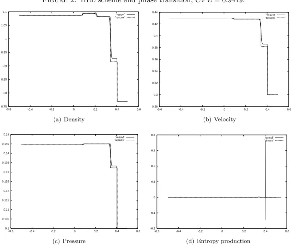
Increasing slightly the CFL number δ leads to the results of Figure 2. This time, the scheme captures another solution. It is possible to affirm that this solution is also an entropy solution by examining the numerical production of entropy in the right shock, where the phase transition holds. This shock is solved on two cells. The entropy production in the right cell is positive. In the left cell, the production is negative. But globally, on the two cells, the production is positive. Thus, at convergence, the solution will be an entropy solution.
CFL δ 0.9418 or 0.9419
number of cells 1000
interval [−1/2, 1/2]
final time t = 0.5
pressure laws (γ1− 1) = 0.6, (γ2− 1) = 0.5
Table 2. computation parameters.
The programs that compute the HLL solution and the exact Liu solution can be downloaded at http://helluy.univ-tln.fr/phasetrans/index.html
To our opinion, it is interesting to note that the construction procedure of the pressure law (46) has an incidence on the exact and numerical solutions of (47). It is also interesting that this behavior is observed with the HLL scheme, known to be highly entropy dissipative.
Intuitively, we explain the existence of several entropy solutions as follows. There are mainly two mechanisms that produce entropy: the admissible shock waves and the phase transition itself. We can imagine that an admissible shock wave, with positive entropy production, is balanced by a non-physical mass transfer between the two phases, with negative entropy production. In this way, we guess that it is possible to construct many entropy solutions to (47), (46).
Of course, it is possible to study directly the Riemann problem for (47), (46), as it is done for example in [19] and [28]. We think however that the underlying entropy optimization that leads to the pressure law (46) helps to understand the behavior of the solutions.
In [2] we have designed a relaxation scheme (different from the HLL scheme) for the approximation of this kind of problems. The main idea is to use a splitting method. Each time step is split into two sub-steps. In the first sub-step, a classical Godunov scheme is employed for a diphasic mixture without phase transition. The mixture variables (the fractions) are convected with the flow. The associated Riemann problem is much easier to solve, as proved in [3], [4]. In a second sub-step, the mixture variables are updated by optimizing the entropy with respect to the mixture variables. The convergence of the solution towards the Liu solution is numerically verified.
We must observe here that other selection criteria have been proposed. For example, with vanishing visco-capillary terms, it can be proved that the relevant solution is made of non-classical shock waves [22], [16]. There is still a debate to know which criterion (Liu’s or visco-capillary) is physically the most relevant.
4.
Miscible mixtures
As it can be checked in (44), the simple model does not present a critical behavior: the saturation curve is infinite in the (T, p) plane. We can wonder if it is possible to obtain a critical behavior (bounded saturation
line) by considering more complex entropies s1 and s2.
We have made such an attempt in [2] to simulate water flows with cavitation. We chose stiffened gas entropies of the form
si= Ciln((εi− Qi− πiτi)τiγi−1) + s0i. (56)
The law is characterized by several physical constants. The parameter Ci is the specific heat of fluid i. The
parameter Qi can be interpreted as a heat of formation. The parameter πi has the dimension of a pressure and
−πi is the minimal pressure for which the sound speed of fluid i vanishes. Although the resulting model can be
made realistic for some ranges of pressures, it appears that it is not possible to get a critical behavior with the stiffened gas entropies. After several attempts with other laws, we now conjecture that our approach has to be slightly modified to model super-critical fluids.
One simple possibility that we will present in Section 4.3 is simply to modify the set of constraints in the optimization problem (22). But before presenting the method, we study the mixture of two miscible fluids.
4.1. Optimization problem
If the two fluids are perfectly miscible, they can both occupy the whole volume. The set of constraints is thus given by (M1, V1, E1, M2, V2, E2) ∈ Q ⇔ (M1, V1, E1) ∈ C, (M2, V2, E2) ∈ C, M1+ M2= M, V16V, V26V, E1+ E2= E. (57)
Consider now the optimization with respect to the volume variables V1and V2in this perfectly miscible case.
The derivatives of Σ with respect to V1and V2are respectively p1/T1and p2/T2. In a model where the pressures
and temperature are >0, the maximum will be reached for a saturated constraint, i.e. for V1= V2= V . As in
the immiscible case, the optimization with respect to the energy E1 implies the temperature equilibrium. After
the optimization with respect to V1, V2, E1, E2, the entropy has thus the form
Σ = S1(M1, V, E1) + S2(M − M1, V, E − E1), (58)
the energy E1depending on the other variables
E1= E1(M, V, E, M1). (59)
The equilibrium pressure is then given by the derivative of the equilibrium entropy p T = ∂Σ ∂V = p1 T1 + 1 T1 ∂E1 ∂V + p2 T2 − 1 T2 ∂E1 ∂V (60)
But at equilibrium, T = T1= T2, and then we recover the Dalton law, which states that the mixture pressure
is the sum of the partial pressures of the two fluids
p = p1+ p2. (61)
Proposition 2. If the mixture is perfectly miscible and if the pressures of the two phases are > 0, then, at
4.2. Example
In this section we study the mixture of two miscible perfect gases. The entropies are
si = ln(ετγi−1). (62)
In the miscible case, the two volume fractions are α1= α2= 1. According to (20) and (15) the mixture entropy
is of the form s(τ, ε, ϕ, z) = ϕs1(τ ϕ, zε ϕ) + (1 − ϕ)s2( τ 1 − ϕ, (1 − z)ε 1 − ϕ ). (63)
A simple computation leads to
s(τ, ε, ϕ, z) = ln ε + (γ − 1) ln τ + ϕ ln z + (1 − ϕ) ln(1 − z)
−γ1ϕ ln ϕ − γ2(1 − ϕ) ln(1 − ϕ),
γ = ϕγ1+ (1 − ϕ)γ2.
(64)
And the optimization with respect to z leads to z = ϕ. Thus s(τ, ε, ϕ) = ln ε + (γ − 1) ln τ
−(γ1− 1)ϕ ln ϕ − (γ2− 1)(1 − ϕ) ln(1 − ϕ),
γ = ϕγ1+ (1 − ϕ)γ2.
(65)
The maximum in ϕ is always reached for the unique solution ϕ0(τ ) of
ϕγ1−1 (1 − ϕ)γ2−1 = µ τ exp(1) ¶γ1−γ2 . (66)
The optimal entropy is s((τ, ε, ϕ0(τ )) and it has no simple expression.
Remark 7. We observe that in this model, there is no saturation curve. Indeed, in contrast with the immiscible
case, it is not possible to define a common pressure to the two components at equilibrium. The transition region from the fluid (1) to the fluid (2) is thus ”diffused” in all the (T, p) plane.
4.3. Critical point
In this section, we propose a simple approach in order to qualitatively model a critical behavior. The idea is to admit progressively a mixture covering of the two components when the energy of the mixture increases. In this way, we will pass from an immiscible model to a miscible one, and we have just seen that in the miscible
model, the saturation zone is ”diffused”. The covering is obtained by altering the volume constraint V1+V26V .
We consider two fluids characterized by their entropy functions, Si(Wi), i = 1, 2. Out of equilibrium, the
mixture entropy is given by (20). However, the volume constraint is intermediate between (22) and (57).
(M1, V1, E1, M2, V2, E2) ∈ Q ⇔ (M1, V1, E1) ∈ C, (M2, V2, E2) ∈ C, M1+ M2= M, E1+ E2= E. V16V, V26V, V1+ V26V + ηE, (67)
The parameter η is small, in such a way that for a small mixture energy E, the mixture behaves like an immiscible one. When the energy increases, the mixture becomes a miscible mixture. More precisely, when
ηE > V , then the constraints Vi≤ V are saturated, and we are exactly in the case of the miscible mixture. We
have pointed out that for a perfectly miscible mixture, there is no more saturation line. We will see that with this model the saturation line is indeed bounded.
Remark 8. It would be interesting to study other volume constraints in (67). For example, we could have
replaced V1+ V26V + ηE by a more general inequality V1+ V26V0(M, V, E) where V0 is a concave and PH1
function. Our choice is based on physical and complexity reasons. We have to study different cases for the optimization problem
S(W ) = max
(W1,W2)∈Q
Σ(W1, W2). (68)
First, the problem can be restated under the form: maximize
Σ = S1(M1, V1, E1) + S2(M − M1, V2, E − E1), (69)
with respect to (M1, V1, V2, E1) under the constraints
V16V, V26V,
V1+ V26V + ηE. (70)
We first study the conditions for equilibrium of the phases. We will consider the case when the two phases exist and are at equilibrium. This means that the maximum of the mixture entropy is reached in the interior of the domain of constraints (at least for the mass and energy: the volume constraint can be saturated, as in the Dalton law).
Proposition 3. If the two phases are present and at equilibrium then
T1= T2= T ,
µ1= µ2= µ.
(71)
Proof. The two phases are present when 0 < M1< M and 0 < E1< E. The result is proved because
∂Σ ∂E1 = 1 T1 − 1 T2 , − ∂Σ ∂M1 = µ1 T1 −µ2 T2 . (72) ¤ We have now to maximize with respect to the volume. Different cases have to be considered. The first
corresponds to ηE ≤ V and the constraint V1+ V26V + ηE alone is saturated. Then, V2= V + ηE − V1.
Proposition 4. If ηE ≤ V and if V2= V + ηE − V1, then at equilibrium, we have also
p1= p2= p.
Proof. Now Σ reads
Σ = S1(M1, V1, E1) + S2(M − M1, V + ηE − V1, E − E1) (73)
The optimality condition reads
∂Σ ∂V1 = p1 T1 −p2 T2 = 0, (74)
A very interesting feature of the proposed simple model is that the temperature, pressure and chemical potential of the equilibrium mixture do not correspond to the common temperatures, pressures and chemical potentials of the two phases. This fact can be stated more precisely thanks to the following proposition.
Proposition 5. If ηE ≤ V and if V2= V +ηE −V1, then at equilibrium, the temperature, pressure and chemical
potential of the mixture are given by
T = T 1 + ηp, p = p 1 + ηp, µ = µ 1 + ηp, (75)
where T , p and µ correspond respectively to the common temperature, pressure and chemical potential of the two components at equilibrium.
Proof. At equilibrium, M1, V1 and E1 depends on M, V, E in such a way that T1 = T2 = T , p1 = p2= p and
µ1= µ2= µ. The mixture equilibrium temperature is then obtained from
1 T = ∂Σ ∂E = ∂ ∂E(S1(M1, V1, E1) + S2(M − M1, V + ηE − V1, E − E1)) M1= M1(M, V, E), V1= V1(M, V, E), E1= E1(M, V, E). (76) It gives 1 T = ∂M1 ∂E µ µ1 T1 −µ2 T2 ¶ +∂V1 ∂E µ p1 T1 −p2 T2 ¶ + ∂E1 ∂E µ 1 T1 − 1 T2 ¶ + ηp2 T2 + 1 T2 (77)
The conditions of equilibrium then give
T = T
1 + ηp.
The other expressions for the pressure and the chemical potential are obtained by similar calculations. ¤
Remark 9. We observe that for the first case, in the “barred” variables, the saturation line is not different from
the saturation line of the immiscible mixture. But the saturation line in the true pressure and temperature is obtained by a transformation (T , p) → (T, p) that maps an unbounded line to a bounded one. For example, the
pressure is bounded by pc= 1/η. This is nothing else than the desired qualitative critical behavior.
We have now to study the transition from an immiscible to a miscible mixture. The next case corresponds
to ηE ≤ V and a maximum reached at a point where V1= V and V2= ηE (and a symmetric case V2= V and
V1= ηE).
Proposition 6. In the case ηE ≤ V , if the maximum is reached for V1= V and V2= ηE then the temperatures
and chemical potentials of the two phases are equal (and noted as before T and µ). The mixture variables at equilibrium are T = T 1 + ηp2 , p = p1 1 + ηp2 , µ = µ 1 + ηp2. (78)
A symmetric formula holds for the case V2= V , V1= ηE.
Proof. Now Σ reads
Σ = S1(M1, V, E1) + S2(M − M1, ηE, E − E1). (79)
At equilibrium, the pressures are not necessarily the same, because the constraint on V1is saturated. The same
kind of computations as in proposition 5 lead to the result. ¤
The last case corresponds to ηE > V . Then necessarily V1= V and V2= V . We are thus in the case of the
perfectly miscible mixture and recover the Dalton law:
Proposition 7. In the case ηE > V , the maximum is reached for V1= V2= V . The temperatures and chemical
potentials of the two phases are equal (and noted as before T and µ). The mixture variables at equilibrium are T = T ,
p = p1+ p2,
µ = µ.
(80)
The computations can be made more precise with particular forms of the entropies and when the optimization problem is stated in intensive variables. The mixture specific entropy is given by
σ = ϕs1( α1 ϕτ, z ϕε) + (1 − ϕ)s2( α2 1 − ϕτ, 1 − z 1 − ϕε). (81)
The specific entropy has to be optimized with the constraints
0 6 z 6 1, 0 6 ϕ 6 1,
0 6 α161, 0 6 α261,
α1+ α261 + ηρε.
(82)
We consider the particular case of two perfect gas laws. The specific entropy is σ = ln ε + (γ − 1) ln τ + ϕ lnz ϕ+ ϕ(γ1− 1) ln α1 ϕ + (1 − ϕ) ln 1 − z 1 − ϕ+ (1 − ϕ)(γ2− 1) ln α2 1 − ϕ, with γ = γ(ϕ) = ϕγ1+ (1 − ϕ)γ2. (83)
We can simplify the expression of the entropy by expressing the temperature equilibrium ∂σ
∂z = 0 ⇔ z = ϕ,
and eliminating the energy fraction z. We find
σ = ln ε + (γ − 1) ln τ
−ϕ(γ1− 1) ln ϕ − (1 − ϕ)(γ2− 1) ln(1 − ϕ)
+ϕ(γ1− 1) ln α1+ (1 − ϕ)(γ2− 1) ln α2,
γ = ϕγ1+ (1 − ϕ)γ2.
This expression has to be optimized for fixed (τ = 1/ρ, ε) with respect to ϕ, α1 and α2. The constraints are
0 6 ϕ 6 1,
0 6 α161, 0 6 α261,
α1+ α261 + ηρε.
(85)
As before, we start to optimize with respect to the volume fractions α1and α2. For this purpose, when ηρε ≤ 1,
we introduce the two mass fractions that will correspond to the saturation of the constraints αi= 0 or αi= 1.
ϕmin= ηρε(γ2− 1) ηρε(γ2− 1) + (γ1− 1) , ϕmax= (γ2− 1) (γ2− 1) + ηρε(γ1− 1) . (86)
If ϕmin6ϕ 6 ϕmax then the maximum in α is
α1= ϕ γ1− 1 γ − 1(1 + ηρε), α2= (1 − ϕ) γ2− 1 γ − 1(1 + ηρε). (87)
If ϕ ≤ ϕminthen the constraint α2≤ 1 is saturated and we have
α1= ηρε,
α2= 1. (88)
If ϕ ≥ ϕmaxthen the constraint α1≤ 1 is saturated and we have
α1= 1,
α2= ηρε. (89)
Finally, when ηρε ≥ 1 the two constraints α1 ≤ 1 and α2 ≤ 1 are saturated and the maximum in α is simply
α1= α2= 1.
The previous computations give the entropy before the optimization with respect to the mass fraction. If ηρε ≤ 1 then:
• If ϕmin6ϕ 6 ϕmax then
σ = ln ε + (γ − 1) lnτ + ηε γ − 1+ ϕ(γ1− 1) ln(γ1− 1) + (1 − ϕ)(γ2− 1) ln(γ2− 1). • If ϕ ≤ ϕminthen σ = ln ε + (γ − 1) ln τ −ϕ(γ1− 1) ln ϕ − (1 − ϕ)(γ2− 1) ln(1 − ϕ) +ϕ(γ1− 1) ln(ηρε). • If ϕ ≥ ϕmaxthen σ = ln ε + (γ − 1) ln τ −ϕ(γ1− 1) ln ϕ − (1 − ϕ)(γ2− 1) ln(1 − ϕ) +(1 − ϕ)(γ2− 1) ln(ηρε).
If ηρε ≥ 1 then
σ = ln ε + (γ − 1) ln τ
−ϕ(γ1− 1) ln ϕ − (1 − ϕ)(γ2− 1) ln(1 − ϕ).
It can be checked that σ is of class C1 with respect to ϕ.
The saturation region is the set of points where the temperature, pressure and chemical equilibriums hold. It implies that its boundary corresponds to the saturation of the volume constraints. It is thus defined by the two equalities ∂σ ∂ϕ(τ2, ε, ϕmin) = 0, ∂σ ∂ϕ(τ1, ε, ϕmax) = 0. (90)
These equalities define two functions τ1(ε) and τ2(ε) and the saturation region in the (τ, ε) plan is defined by
τ1(ε) ≤ τ ≤ τ2(ε). (91)
Defining the same constant κ as in (44) κ = exp µ 1 −(γ1− 1) ln(γ1− 1) − (γ2− 1) ln(γ2− 1) γ1− γ2 ¶ , we find τ2= κ(γ2− 1) − γ2− 1 γ1− 1ηε, τ1= κ(γ1− 1) − γ1− 1 γ2− 1 ηε. (92)
The two curves τ1 and τ2 intersect at the critical point, for which ηε/τ = 1. Then the critical specific volume
τc satisfies κ = τc(γ11−1+γ21−1).
It is more classical to express τ1 and τ2 with respect to the pressure. It is easily done using the equilibrium
of temperatures and pressures in the saturation zone and on its boundary (see Proposition 5)
T1= T2= T = ε1= ε2, ε = ϕε1+ (1 − ϕ)ε2= T , p1= p2= p, T /p = T /p = κ, T = T 1 + ηp, p = p 1 + ηp.
In the saturation region, we thus have
ε = κ p
1 − ηp. (93)
In the (τ, p) plane, the left and right boundaries of the saturation region are
τ1= κ(γ1− 1) − γ2− 1 γ1− 1 ηκ p 1 − ηp, τ2= κ(γ2− 1) − γ1− 1 γ2− 1 ηκ p 1 − ηp. (94)
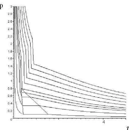
It is not possible to give an explicit form of the pressure law. But by simple numerical computations, it is possible for example to draw the isothermal lines in the (τ, p) plane. They are represented on Figure 3
with γ1= 1.4 and γ2 = 1.1. The Maple worksheet that permits to draw the Figure 3 is also provided on the
above-mentioned web page.
The main qualitative behavior near the critical point is recovered: • bounded saturation region in the (τ, p) plane;
• existence of a bounded saturation line in the (T, p) plane;
• the pressure is constant along the isothermal lines in the saturation region.
However some features, found in the van der Waals model for example [19], [9], are still missing:
• ∂p∂τ 6= 0 at the intersection of the two curves τ1 and τ2;
• p(τ2) is decreasing. For real material is should be increasing (but in practice, it is almost vertical);
• The pressure admits a jump on the line ηε/τ = 1 instead of being continuous.
Let us repeat that our model is very simple. It is certainly possible to add more details to each single fluid entropy law as: heat capacities, heat of formation, reference entropies. Maybe it is then possible to recover the missing features.
Let us also mention that it’s worth it because our model is also valid out of equilibrium unlike the van der Waals model that is a purely equilibrium model.
Conclusion
In this work, we have proposed a review of some results of the thermodynamics of mixtures. The computation of the equilibrium of two phases can be formulated as a constrained optimization problem on the mixture entropy. Many results are classical, but to our opinion, are not so clearly stated in the literature. Some remarks seem to be new:
• it appears that the equilibrium entropy is the sup-convolution of the entropies of the two phases. This can lead to many interesting applications related to fast Legendre transform algorithms;
• the isobaric law and the Dalton law can be rigorously proved by changing the constraints in the entropy optimization problem;
• one can define in a very natural way an entropy, and thus a pressure and a temperature, for a mixture out of equilibrium. We have thus to our disposal models for the dynamics of the phase transition. It would be interesting to compare the physical validity of such models with the classical model of metastability of van der Waals.
We have seen that the optimization problem is much easier to understand, on the theoretical side, when it is stated in extensive variables. However, for CFD applications and the coupling with Euler equations, it is necessary to state it in intensive variables.
Finally, we have given a tentative modelling of a super-critical fluid. We proposed a very simple modification of the constraints in the optimization of the entropy. With this modification, the mixture is more and more miscible when the energy increases. Some qualitative properties of super-critical fluids are recovered: bounded saturation line, horizontal isotherms in the saturation zone, etc. Investigations are still needed to obtain a more precise model for super-critical fluids.
References
[1] Gr´egoire Allaire, S´ebastien Clerc, and Samuel Kokh. A five-equation model for the simulation of interfaces between compressible fluids. J. Comput. Phys., 181(2):577–616, 2002.
[2] T. Barberon and Helluy. Finite volume simulation of cavitating flows. Computers and Fluids, 34(7):832–858, 2005.
[3] T. Barberon, P. Helluy, and S. Rouy. Practical computation of axisymmetrical multifluid flows. International Journal of Finite Volumes http: // averoes. math. univ-paris13. fr/ IJFV , 1(1):1–34, 2003.
[4] Thomas Barberon and Philippe Helluy. Finite volume simulations of cavitating flows. In Finite volumes for complex applica-tions, III (Porquerolles, 2002), pages 441–448 (electronic). Lab. Anal. Topol. Probab. CNRS, Marseille, 2002.
[5] Fran¸cois Bouchut. A reduced stability condition for nonlinear relaxation to conservation laws. J. Hyperbolic Differ. Equ., 1(1):149–170, 2004.
[6] Yann Brenier. Averaged multivalued solutions for scalar conservation laws. SIAM J. Numer. Anal., 21(6):1013–1037, 1984. [7] Yann Brenier. Un algorithme rapide pour le calcul de transform´ees de Legendre-Fenchel discr`etes. C. R. Acad. Sci. Paris S´er.
I Math., 308(20):587–589, 1989.
[8] H. B. Callen. Thermodynamics and an introduction to thermostatistics, second edition. Wiley and Sons, 1985.
[9] F. Caro. Mod´elisation et simulation num´erique des transitions de phase liquide-vapeur. PhD thesis, ´Ecole Polytechnique, Paris, France, november 2004.
[10] G. Chanteperdrix, P. Villedieu, and Vila J.-P. A compressible model for separated two-phase flows computations. In ASME Fluids Engineering Division Summer Meeting. ASME, Montreal, Canada, July 2002.
[11] Gui Qiang Chen, C. David Levermore, and Tai-Ping Liu. Hyperbolic conservation laws with stiff relaxation terms and entropy. Comm. Pure Appl. Math., 47(6):787–830, 1994.
[12] J.-P. Croisille. Contribution `a l’´etude th´eorique et `a l’approximation par ´el´ements finis du syst`eme hyperbolique de la dynamique des gaz multidimensionnelle et multiesp`eces. PhD thesis, Universit´e Paris VI, France, 1991.
[13] St´ephane Dellacherie. Relaxation schemes for the multicomponent Euler system. M2AN Math. Model. Numer. Anal., 37(6):909– 936, 2003.
[14] L. C. Evans. Entropy and partial differential equations.
http://math.berkeley.edu/~evans/entropy.and.PDE.pdf, 2004.
[15] A. Harten, P. D. Lax, and B. Van Leer. On upstream differencing and Godunov-type schemes for hyperbolic conservation laws. SIAM Rev., 25(1):35–61, 1983.
[16] B. T. Hayes and P. G. Lefloch. Nonclassical shocks and kinetic relations: strictly hyperbolic systems. SIAM J. Math. Anal., 31(5):941–991 (electronic), 2000.
[17] Jean-Baptiste Hiriart-Urruty. Optimisation et analyse convexe. Math´ematiques. [Mathematics]. Presses Universitaires de France, Paris, 1998.
[18] Jean-Baptiste Hiriart-Urruty and Claude Lemar´echal. Fundamentals of convex analysis. Grundlehren Text Editions. Springer-Verlag, Berlin, 2001.
[19] S. Jaouen. ´Etude math´ematique et num´erique de stabilit´e pour des mod`eles hydrodynamiques avec transition de phase. PhD thesis, Universit´e Paris VI, November 2001.
[20] L. Landau and Lifchitz E. Physique statistique. Physique th´eorique. Ellipses, Paris, 1994.
[21] P.D. Lax. Hyperbolic systems of conservation laws and the mathematical theory of shock waves. In CBMS Regional Conf. Ser. In Appl. Math. 11, Philadelphia, 1972. SIAM.
[22] P. G. LeFloch and C. Rohde. High-order schemes, entropy inequalities, and nonclassical shocks. SIAM J. Numer. Anal., 37(6):2023–2060, 2000.
[23] Randall J. LeVeque and Marica Pelanti. A class of approximate Riemann solvers and their relation to relaxation schemes. J. Comput. Phys., 172(2):572–591, 2001.
[24] T. P. Liu. The Riemann problem for general systems of conservation laws. J. Diff. Equations., 56:218–234, 1975. [25] Y. Lucet. A fast computational algorithm for the Legendre-Fenchel transform. Comput. Optim. Appl., 6(1):27–57, 1996. [26] Yves Lucet. Faster than the fast Legendre transform, the linear-time Legendre transform. Numer. Algorithms, 16(2):171–185
(1998), 1997.
[27] P.-A. Mazet and F. Bourdel. Multidimensional case of an entropic variational formulation of conservative hyperbolic systems. Rech. A´erospat., (5):369–378, 1984.
[28] R. Menikoff and B. J. Plohr. The Riemann problem for fluid flow of real materials. Rev. Modern Phys., 61(1):75–130, 1989. [29] B. Perthame. Boltzmann type schemes for gas dynamics and the entropy property. SIAM J. Numer. Anal., 27(6):1405–1421,
1990.
[30] R. Saurel and R. Abgrall. A multiphase Godunov method for compressible multifluid and multiphase flows. J. Comput. Phys., 150(2):425–467, 1999.
Figure 1. HLL scheme and phase transition, CF L = 0.9418. 0.75 0.8 0.85 0.9 0.95 1 1.05 1.1 -0.6 -0.4 -0.2 0 0.2 0.4 0.6 ’resuvf’ ’resuex’ (a) Density 0.28 0.3 0.32 0.34 0.36 0.38 0.4 0.42 0.44 -0.6 -0.4 -0.2 0 0.2 0.4 0.6 ’resuvf’ ’resuex’ (b) Velocity 0.1 0.105 0.11 0.115 0.12 0.125 0.13 0.135 0.14 0.145 0.15 -0.6 -0.4 -0.2 0 0.2 0.4 0.6 ’resuvf’ ’resuex’ (c) Pressure -0.02 0 0.02 0.04 0.06 0.08 0.1 0.12 0.14 0.16 0.18 -0.5 -0.4 -0.3 -0.2 -0.1 0 0.1 0.2 0.3 0.4 0.5 ’resuvf’ ’resuex’ (d) Entropy production
Figure 2. HLL scheme and phase transition, CF L = 0.9419. 0.75 0.8 0.85 0.9 0.95 1 1.05 1.1 -0.6 -0.4 -0.2 0 0.2 0.4 0.6 ’resuvf’ ’resuex’ (a) Density 0.28 0.3 0.32 0.34 0.36 0.38 0.4 0.42 0.44 -0.6 -0.4 -0.2 0 0.2 0.4 0.6 ’resuvf’ ’resuex’ (b) Velocity 0.1 0.105 0.11 0.115 0.12 0.125 0.13 0.135 0.14 0.145 0.15 -0.6 -0.4 -0.2 0 0.2 0.4 0.6 ’resuvf’ ’resuex’ (c) Pressure -0.2 -0.1 0 0.1 0.2 0.3 0.4 -0.6 -0.4 -0.2 0 0.2 0.4 0.6 ’stnsvf’ ’stnsex’ (d) Entropy production