INTEGRATING WAVE AND TIDAL CURRENT POWER: Case Studies Through Modelling and Simulation

HAL Id: hal-01265985

https://hal.archives-ouvertes.fr/hal-01265985

HAL is a multi-disciplinary open access archive for the deposit and dissemination of sci-entific research documents, whether they are pub-lished or not. The documents may come from teaching and research institutions in France or abroad, or from public or private research centers.

L’archive ouverte pluridisciplinaire HAL, est destinée au dépôt et à la diffusion de documents scientifiques de niveau recherche, publiés ou non, émanant des établissements d’enseignement et de recherche français ou étrangers, des laboratoires publics ou privés.

INTEGRATING WAVE AND TIDAL CURRENT

POWER: Case Studies Through Modelling and

Simulation

M. Santos, F. Salcedo, D. Ben Haim, J. L. Mendia, P. Ricci, J.L. Villate, J.

Khan, D. Leon, S. Arabi, A. Moshref, et al.

To cite this version:

M. Santos, F. Salcedo, D. Ben Haim, J. L. Mendia, P. Ricci, et al.. INTEGRATING WAVE AND TIDAL CURRENT POWER: Case Studies Through Modelling and Simulation . [Research Report] Document No: T0331, International Energy Agency Implementing Agreement on Ocean Energy Sys-tems 2011. �hal-01265985�

International Energy Agency Implementing Agreement on

Ocean Energy Systems

I

NTEGRATING

W

AVE AND

T

IDAL

C

URRENT

P

OWER

:

Case Studies Through Modelling and Simulation

March 2011

A report prepared by

Tecnalia, Powertech Labs and HMRC

As part of the OES-IA Annex III Collaborative Task on

Integration of Ocean Energy Plants into Electrical Grids

I

W

T

C

P

:

Case Studies Through Modelling and Simulation

OES-IA Document No: T0331

Operating Agent:

Gouri Bhuyan, Powertech Labs, Canada

Authors:

Maider Santos Múgica, Tecnalia, Spain Fernando Salcedo Fernandez, Tecnalia, Spain David Ben Haim, Tecnalia, Spain

Joseba Lopez Mendia, Tecnalia, Spain Pierpaolo Ricci, Tecnalia, Spain

Jose Luis Villate Martínez, Tecnalia, Spain Jahangir Khan, Powertech Labs, Canada Daniel Leon, Powertech Labs, Canada Saeed Arabi, Powertech Labs, Canada Ali Moshref, Powertech Labs, Canada Gouri Bhuyan, Powertech Labs, Canada Anne Blavette, HMRC, Ireland

Dara O’Sullivan, HMRC, Ireland Ray Alcorn, HMRC, Ireland

Availability of the Report:

A PDF file of this report is available at: www.iea-oceans.org Suggested Citation for the Report:

M. Santos, F. Salcedo, D. Ben Haim, J. L. Mendia, P. Ricci, J.L. Villate, J. Khan, D. Leon, S. Arabi, A. Moshref, G. Bhuyan, A. Blavette, D. O’Sullivan, R. Alcorn; (2011). Integrating Wave and Tidal Current Power: Case Studies through Modelling and Simulation, A report prepared jointly by Tecnalia (Spain), Powertech Labs (Canada) and HMRC (Ireland) for the OES-IA. Available: www.iea-oceans.org

DISCLAIMER

The OES-IA, also known as the Implementing Agreement on Ocean Energy Systems, functions within a framework created by the International Energy Agency (IEA). Views, findings and publications of the OES-IA do not necessarily represent the views or policies of the IEA Secretariat or of all its individual member countries.

The reader is encouraged to consult with relevant references and external sources.

Various device names, technologies, software and hardware systems cited in this report may represent trade names and the TM symbol is not used. These trademarks should be treated accordingly.

FOREWARD

The International Energy Agency (IEA) is an autonomous body within the framework of the Organization of Economic Co-operation and Development (OECD), which carries out a comprehensive program of energy co-operation among different countries. The Implementing Agreement on Ocean Energy Systems (OES-IA) is one of the several IEA collaborative agreements within the renewable energy domain.

This report has been prepared under the supervision of the Operating Agent for the OES-IA Annex III on Integration of Ocean Energy Plants into Distribution and Transmission Grids based on cost-shared and task-shared collaborative activities. The report provides valuable information to various stakeholders, including the members of the OES-IA, and presents case studies demonstrating integration of wave and tidal current power generating plants to distribution grids, as well as to a larger power system at the transmission level, considering various long-term scenarios.

Dr. John Huckerby Dr. Gouri Bhuyan

ACKNOWLEDGEMENTS

The OES-IA member countries that are participating in the work program of the Annex are Canada, Ireland, United Kingdom, Spain and New Zealand. Funding for the overall management of the Annex activities was provided by Powertech Labs, the UK Department of Energy and Climate Change (DECC), Tecnalia of Spain and AWATEA of New Zealand.

The participating organisations and the corresponding enabling funding contributors for this Annex are as follows:

Powertech Labs with direct and indirect financial contribution from BC Hydro and Powertech Labs, Canada; Bonneville Power Administration (BPA), USA; Oregon Wave Energy Trust (OWET), USA; and Asia Pacific Partnership (APP) Program of Environment Canada.

Hydraulic Maritime Research Centre (HMRC) with financial contribution from the Sustainable Energy Authority of Ireland (SEAI), and Science Foundation Ireland under the Charles Parsons Initiative.

Tecnalia with direct financial contribution from Ente Vasco de la Energía (EVE). The Tecnalia authors wish to acknowledge Ana Morales from DIgSILENT Iberica, S.L. for her help with the simulation models.

The Powertech authors acknowledge contributions from John Schaad and Sara Sundborg of BPA; Mark Tallman and Dennis Desmarais of PacifiCorp; Pat Ashby of Tillamook PUD; Mike Wilson and Joseph Monsanto of Central Lincoln PUD; Dave Sabala and Todd Sherwood of Douglas Electric Cooperative; Kevin Watkins of PNGC Power; Vickie VanZandt of Ecofys; and Justin Klure and Therese Hampton of Pacific Energy Venture for enabling the case study, reported in section 3.3 of this report. Also, contributions from Kang Won Lee of DAEHWA Power Engineering Co., Ltd., Republic of Korea, and Seung Hee Kim of KEPCO, Republic of Korea, towards providing the required information on the Korean system for the case study discussed in section 3.4 of this report are acknowledged. Technical contributions by Frederic Howell and Xi Lin from Powertech Labs Inc. for providing assistance toward developing and implementing the tidal current and wave energy conversion models into DSATools are greatly appreciated.

Thanks to James Griffiths for his technical help to the HMRC team. Valuable inputs provided by Michael Egan during the program as well as in drafting and producing certain part of this report are acknowledged.

Special thanks to Hannele Holttinen of VTT Technical Research Centre of Finland, and John Pease, John Schaad, Nic Peck and Paul Fiedler of BPA for their expert review of the document. Also, efforts made by Ana Brito Melo of Wave Energy Centre, Portugal, and John Huckerby of AWATEA, New Zealand, in reviewing the report are very much appreciated.

E

XECUTIVE

S

UMMARY

Ocean renewable energy is an emerging resource option. In the long term, ocean renewable energy has the potential to provide a significant share of global energy needs. Currently, some of the conversion technologies for harnessing variable wave and tidal current energy resources are reaching commercial stage. Several pilot projects, having sizes upto 2 MW, are operating in various parts of the world. Also multi-MW wave and tidal current energy farms are being developed. Identification of the near- and longer-term technical potential of wave and tidal current resources that could be integrated to existing and future electricity infrastructure in a region is an important step towards developing integrated long-term energy planning for the region and relevant policy instruments to realize the potential.

During the past three years, a collaborative project related to integration of wave and tidal current energy into electrical systems (known as Annex III) was carried out under the umbrella of the International Energy Agency’s Implementing Agreement on Ocean Energy Systems (OES-IA) (www.iea-oceans.org). Following the completion of the Work Packages 1 and 2 under the Annex III of IEA’s Ocean Energy Implementing Agreement, a number of landmark activities took place within the emerging global ocean energy sector. This report summarizes the work performed through the Work Package 3 activities. The report provides insight into the grid integration of wave and tidal current resources, particularly through case studies spanning a wide range of scenarios. In particular, the following case studies are presented in this report:

Case Study Country Generation Level (MW) Time Horizon Project Type Conversion Device Case Study Focus Integration Level Biscay Marine Energy Platform (bimep) Spain 20 Near-term (2011) Multi-unit pilot Generic

wave Power quality Distribution

Belmullet Wave Test Site Ireland 5 Near-term (2011) Multi-unit pilot Generic wave

Power quality Distribution Oregon

Coasts USA ~500 Long-term

(~2019)

Wave

farm Generic wave System planning and deployment potential, adequacy of on-shore infrastructure Transmission Korean Country-wide Republic

of Korea ~ 2000 Long-term (~2022) Tidal and wave farm Generic tidal and wave System planning and deployment potential Transmission

Prior to discussing these case studies, a number of generic power system related aspects (such as system control, stability, power quality, grid codes, etc.) are highlighted in this report. In addition, brief discussions are presented on wave and tidal resource variability/predictability, offshore farm layout, system control and characteristics, plant location (in contrast to the location of load centers, network topology, etc.).

The following summary can be drawn upon from the studied cases: Distribution Integration (Spain, Ireland):

 The developed case studies for distribution systems indicate that there are no

significant technical barriers to the grid connection of a wave farm, both at Biscay Marine Energy Platform (bimep) (20 MW) and at the Belmullet test site (5 MW). This is a positive outcome, especially as, apart from the study focused on the effect of device aggregation, all the other studies were performed with no phase shift applied between the power output of the different devices’ power output, which represents the worst case scenario for the power fluctuations approach.

 In the case of bimep, the wave farm effects on the connection point are not

significant since the associated distribution grid is strong. With an increasing penetration level of marine renewable energy, the achievement of acceptable power quality issues will be more complex and specific studies on reactive power control and compensation (i.e., flexible AC transmission system or FACTS) will be mandatory.

 Some minor concerns in terms of power quality and voltage variation arise at

Belmullet for the wave farms with power capacity exceeding 3 MW and with extreme power fluctuations (zero to peak value at each cycle). This situation occurs when connecting devices have no energy storage capacity and with minimal smoothing from device aggregation.

 The system power losses were shown to be larger for a system with fluctuating

power output, compared with a non-fluctuating system with the same mean output. This has an impact on component ratings and special attention must be paid to thermal design when considering fluctuating power flows.

 The local network of Belmullet is currently used to distribute power to a small

population from remote power plants. The integration of a wave farm to this grid radically alters the operating envelope of the local circuit breakers, as shown by the fault study.

Transmission Integration (USA, Republic of Korea):

 Considering simultaneous wave energy power generation from selected target areas

along the coast of Oregon, the aggregated capacity transfer limit from west to east is found to be approximately 430 MW. This threshold of capacity addition is a

conservative estimate. A set of twelve points of interconnection (POI)s were evaluated and the capacity levels were found to be highly diverse (from 5 MW to 480 MW, depending on the POI).

 Under the scope of this study, with its underlying assumptions and criteria, it has

been identified that the primary limiting factor is line overloading. Further studies with broader scope may provide more insight considering the Pacific NW coastal region (Washington, British Columbia, California, in addition to Oregon under

longer time horizons), as well as the use of high voltage DC transmission (HVDC), flexible AC transmission system (FACTS) devices, effects of special contingencies and protection schemes.

 With regard to tidal and wave power integration in the Korean electricity network,

voltage security, transient security and small signal stability analyses for the years 2017 and 2022, under both peak and light loading conditions, have been carried out. It was assumed that, before 2017, Jeju Island would be connected to the Korean mainland through two high voltage direct current (HVDC) submarine transmission links, totalling a maximum capacity of 700 MW in either direction.

 Two locations of ocean wave energy generation into Jeju Island and four locations

of tidal current power generation into the Korean mainland were considered. The maximum new generation injections into the island and mainland were 1000 MW and 620 MW, respectively, to be dispatched against forecasted load increases in certain areas of the mainland. The voltage and transient security limitations observed from the case study could be removed by adding a parallel 765 kV circuit.

These case studies provide insights into a broad range of project scenarios, integration challenges, device types, time-horizons and technical aspects. Power system modelling and simulation have been used as vehicles for these assessments.

Based on the knowledge gained through the activities of this Annex, recommendations for subsequent collaboration on relevant topics have been made.

T

ABLE OF

C

ONTENTS

1.3  Variability and Intermittency of Wave and Tidal Current Resources ... 23 

1.4  Present Generation Characteristics of Wave and Tidal Current Conversion Processes ... 26 

1.5  Power System Stability and Control ... 28 

1.5.1  Power System Control ... 31 

1.5.2  Power System Inertia ... 33 

1.5.3  Power System Stability Problem ... 33 

1.5.4  Classification of Stability ... 34 

1.6  Power Quality ... 36 

1.6.1  Local Impact and Power Quality Issues ... 38 

1.7  Grid Connection Codes ... 41 

1.7.1  Voltage and Reactive Power Control ... 43 

1.7.2  Frequency Control ... 44 

1.7.3  Fault Ride-Through Capability ... 47 

1.7.4  Relay Protections ... 48 

1.8  Interconnection Standards and Guidelines ... 49 

1.8.1  IEEE Standard for Interconnecting Distributed Resources with Electric Power Systems (IEEE 1547/2003) ... 49 

1.10  Power System Simulation Tools ... 51 

2  Grid-connected Pilot Plants and Future Grid Integration Issues ... 54 

2.1  Grid-Connected Pilot Plants ... 54 

2.1.1  Predictability, Dispatchability and Capacity Factor ... 59 

2.2  Layout of devices ... 62 

2.2.1  Basic Structures of Ocean Farm Electrical Systems ... 62 

2.2.2  Cluster Array Types ... 64 

2.2.3  Integration Architectures ... 66 

2.2.4  Electrical Transmission Options ... 68 

2.2.5  Generation Units and Conversion Systems ... 73 

2.3  Characteristics of Conversion Systems and control ... 76 

2.3.1  System Modelling Detail Level ... 77 

2.3.2  Control of Oscillating Wave Energy Converters ... 78 

2.3.3  Reactive Power Compensation Technologies for Control of Grid Integration ... 79 

2.4  Site ... 81 

2.4.1  Strong Grid and Weak Grid ... 81 

2.4.2  National Electric Power System Maps ... 83 

2.4.3  Biscay Marine Energy Platform ... 102 

2.4.4  Belmullet Wave Energy Test Site ... 103 

3  Case Study ... 105 

3.1  Distribution System: Basque Country Case Study ... 105 

3.1.1  Electrical Network Modelling ... 106 

3.1.2  WEC Modelling ... 109 

3.1.3  Distribution Code Requirements ... 110 

3.1.4  Load Flow ... 111 

3.1.5  Power Losses ... 114 

3.1.6  Aggregation of Devices ... 114 

3.1.8  Voltage Issues ... 116 

3.1.9  Conclusion ... 116 

3.2  Distribution System: Ireland Case Study ... 118 

3.2.1  Electrical Network Modelling ... 118 

3.2.2  WECs Modelling ... 119 

3.2.3  Distribution Code Requirements ... 120 

3.2.4  Load Flow ... 120 

3.2.5  Power Losses ... 121 

3.2.6  Aggregation of Devices ... 126 

3.2.7  Contingency Analysis ... 127 

3.2.8  Voltage Limits and Voltage Variations ... 127 

3.2.9  Conclusion ... 135 

3.3  Transmission System: Oregon (USA) Case Study ... 136 

3.3.1  Introduction ... 136 

3.3.2  Base Case Description ... 137 

3.3.3  Dynamic Modelling of Wave Energy Converter ... 141 

3.3.4  Scenario Setup ... 145 

3.3.5  Steady-State/Voltage-Security Analysis ... 149 

3.3.6  Time Domain/Transient Security Analysis ... 151 

3.3.7  Conclusion ... 154 

3.4  Transmission System: The Republic of Korea Case Study ... 155 

3.4.1  Introduction ... 155 

3.4.2  Base Case Descriptions ... 156 

3.4.3  Dynamic Modelling of Tidal Current Energy Converter ... 156 

3.4.4  Scenario Setup ... 159 

3.4.5  Steady-State/Voltage-Security Assessments ... 160 

3.4.6  Time Domain/Transient Security Assessment ... 162 

3.4.7  Small Signal Stability Analysis ... 162 

4  Discussion and Recommendations ... 164 

4.1  Summary ... 164 

4.1.1 Predictability of Wave and Tidal Current Resources ... 164 

4.1.2 Dispatchability ... 165 

4.1.3 Capacity Factor of Wave and Tidal Current Power Plants ... 165 

4.1.4 Power quality ... 165 

4.1.5 Interconnection guidelines ... 166 

4.1.6 Integrated system scenario analyses ... 167 

4.1.7 Integration of the Technologies with Storage into NIA/Autonomous Systems ... 168 

4.2  Recommendations for Future Collaboration... 169 

4.2.1 Pilot project information collection and dissemination ... 169 

4.2.2 Power quality impact and system design ... 169 

4.2.3 Dynamic model validation ... 169 

4.2.4 Device and interconnection guidelines ... 169 

4.2.5 Integrated system scenario assessment for a larger power system ... 169 

4.2.6 Development methodology to optimise size of demonstration and storage for NIA/autonomous systems ... 170 

L

IST OF

F

IGURES

Figure 1.1: Ocean Energy Conversion Systems (Tidal and Wave) [1]. ... 26 

Figure 1.2: Subsystems of a power system and associated controls [13] ... 30 

Figure 1.3: Load balance and scheduling [1]. ... 31 

Figure 1.4: Power system operating states [13] ... 32 

Figure 1.5: Classification of power system stability [13]. ... 35 

Figure 1.6: Classical model of the power system [17]. ... 36 

Figure 1.7: Modern model of power system [17]. ... 37 

Figure 1.8: Possible grid impact issues pertaining to ocean energy systems [1]... 38 

Figure 1.9: Typical limiting curve for reactive power [22]. ... 43 

Figure 1.10: Typical frequency controlled regulation of active power [24]. ... 44 

Figure 1.11: Summary of frequency control requirements imposed by several countries grid codes ([21], [22], [23], [31], [32], [33]). ... 46 

Figure 1.12: Curve of the voltage in function of the time at the connection point, defining the voltage dip area [32] ... 47 

Figure 1.13: Operational area (in grey) during fault and recovery periods in function of the voltage at the connection point [33] ... 48 

Figure 2.1: Examples of potential wave farms spatial configurations ... 63 

Figure 2.2: Interaction diagram: Main factors influencing the offshore farm layout design ... 63 

Figure 2.3: Main types of clustering for marine energy farms [64] ... 65 

Figure 2.4: Interconnecting cables routes for AC and DC technology ... 65 

Figure 2.5: DC series cabling ... 66 

Figure 2.6: Integration topologies [65] ... 67 

Figure 2.7: HVAC transmission - small farm (T1). ... 69 

Figure 2.8: HVAC transmission – large farm (T2). ... 69 

Figure 2.9: HVDC transmission – large AC-clustered farm (T3) ... 71 

Figure 2.10: HVDC transmission – large DC-clustered farm 1 (T4) ... 71 

Figure 2.12: HVDC transmission – small DC-clustered farm (T6) ... 72 

Figure 2.13: Generation units configurations used in marine offshore energy ... 74 

Figure 2.14: Typical ocean energy conversion process ... 76 

Figure 2.15: Short-circuit diagram ... 81 

Figure 2.16: X/R ratio [87]. ... 83 

Figure 2.17: Population distribution in England and Wales [88] and in Scotland [89] ... 84 

Figure 2.18: Electric power transmission grid in United Kingdom [90] ... 84 

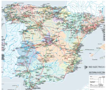
Figure 2.19: Population distribution in Spain [67] ... 85 

Figure 2.20: Electric power transmission grid in Spain [91] ... 85 

Figure 2.21: Population distribution in Portugal [92] ... 86 

Figure 2.22: Electric power transmission grid in Portugal [93] ... 86 

Figure 2.23: Population distribution in Ireland [67] ... 87 

Figure 2.24: Electric power transmission grid in Ireland [94]. ... 87 

Figure 2.25: Population distribution as of July 1, 2007 in Canada [95] ... 88 

Figure 2.26: Canada-USA interconnected electricity network [96] ... 88 

Figure 2.27: Population distribution in United States [97]. ... 89 

Figure 2.28: Electric power transmission grid in the United States [98]. ... 89 

Figure 2.29: Population distribution in the Republic of Korea [99]. ... 90 

Figure 2.30: Electric power transmission grid in the Republic of Korea [100]. ... 90 

Figure 2.31: Population distribution in Denmark [101]. ... 91 

Figure 2.32: Electric power transmission grid in Denmark [98]. ... 91 

Figure 2.33: Population distribution in Japan [67]. ... 92 

Figure 2.34: Electric power transmission grid in Japan [98]. ... 92 

Figure 2.35: Population distribution in Belgium [101]. ... 93 

Figure 2.36: Electric power transmission grid in Belgium [102]. ... 93 

Figure 2.37: Population distribution in Germany [67] ... 94 

Figure 2.38: Electric power transmission grid in Germany [98]. ... 94 

Figure 2.39: Population distribution in Mexico [67]. ... 95 

Figure 2.41: Population distribution in Norway [101] ... 96 

Figure 2.42: Electric power transmission grid in Norway [98] ... 96 

Figure 2.43: Population distribution in Italy [103] ... 97 

Figure 2.44: Electric power transmission grid in Italy [98] ... 97 

Figure 2.45: Population distribution in New Zealand [67] ... 98 

Figure 2.46: Electric power transmission grid in New Zealand [98] ... 98 

Figure 2.47: Population distribution in Sweden [104] ... 99 

Figure 2.48: Electric power transmission grid in Sweden [105] ... 99 

Figure 2.49: Population distribution in Australia [106] ... 100 

Figure 2.50: Electric power transmission grid in Australia [107] ... 100 

Figure 2.51: Population distribution in South Africa [67] ... 101 

Figure 2.52: Electric power transmission grid in South Africa [98] ... 101 

Figure 2.53: Location of bimep ... 102 

Figure 2.54: Aerial view of bimep test zone with planned cable routes [108]. ... 103 

Figure 2.55: Conceptual layout of the facility [109]. ... 104 

Figure 3.1: bimep architecture. ... 106 

Figure 3.2: Simulated grid model ... 108 

Figure 3.3: Fault ride-through capability ... 111 

Figure 3.4: Maximum loading level ... 112 

Figure 3.5: Voltage profile from the WEC 1 to the PCC for SC and SG ... 113 

Figure 3.6: Voltage profile from the WEC 4 to the PCC for SC and SG ... 113 

Figure 3.7: Total losses (MW) and efficiency (%). ... 114 

Figure 3.8: Power and voltage variations ... 115 

Figure 3.9: Voltage profile (pu) when a voltage sag occurs at the PCC for different wave farm power (a) 1.1 MW (b) 6 MW (c) 7.5 MW (d) 12 MW ... 117 

Figure 3.10: Voltage profile (pu) when a voltage sag occurs at the PCC for different wave farm power (a) 1.1 MW (b) 7.5 MW ... 117 

Figure 3.11: Grid model ... 119 

Figure 3.13: Distribution of power loss with respect to the electrical components (load

flow) ... 122 

Figure 3.14: Power output of generator SG 1 ... 123 

Figure 3.15: Efficiency of the network ... 124 

Figure 3.16: Standard deviation of Pin and Pout ... 125 

Figure 3.17: Difference between the standard deviation of Pin and Pout ... 125 

Figure 3.18: Maximum voltage standard deviation ... 127 

Figure 3.19: Voltage at the 10 kV bus versus number of generation units lost... 127 

Figure 3.20: Maximum voltage values at the 10 kV, 20 kV and 38 kV buses ... 128 

Figure 3.21: Minimum voltages ... 129 

Figure 3.22: Maximum allowed power fluctuation amplitude ... 130 

Figure 3.23: Voltage at the PCC for wave farm capacity of 1 MW, 3 MW and 5 MW (Scenario a) ... 131 

Figure 3.24: Voltage at the PCC and at two generator terminals for a wave farm capacity of 3 MW (Scenario a) ... 131 

Figure 3.25: Voltage at the PCC and at two generator terminals with no short-circuit clearance for a wave farm capacity of 3 MW (scenario a) ... 132 

Figure 3.26: Reactive power in MVAR of a single generator and voltage at the PCC in pu ... 133 

Figure 3.27: Speed in pu of Generator 1 ... 133 

Figure 3.28: Voltage at the PCC for wave farm capacity of 1 MW, 3 MW and 5 MW (Scenario b) ... 134 

Figure 3.29: Northwest area and the neighbouring authorities ... 138 

Figure 3.30: Oregon coast and the transmission network (existing) ... 140 

Figure 3.31: Coastal regions and power flow directions (projected, but no wave power generation added) ... 140 

Figure 3.32: Outline of ocean wave energy converter model ... 142 

Figure 3.33 Example power matrix of a hinged contour device ... 144 

Figure 3.34: Transfers and points of interconnection ... 147 

Figure 3.35: WEC implementation in powerflow base cases ... 149 

Figure 3.37: Ocean wave generator speed observed at all POIs ... 152 

Figure 3.38: Generator relative rotor angles for units located near the wave power plants ... 153 

Figure 3.39: A map of the power grid of the Republic of Korea in 2009 ... 155 

Figure 3.40: Diversity of tidal current energy conversion systems ... 157 

Figure 3.41: Tidal current device power conversion subsystems ... 157 

Figure 3.42: Model elements of a tidal current conversion system ... 158 

Figure 3.43: Tidal current device model blocks, as implemented in power system analysis software ... 159 

L

IST OF

T

ABLES

Table 1.1: Timescale of natural cycle of renewable energy processes [4] ... 23 

Table 1.2: Ocean device specific factors affecting the connection configuration ... 40 

Table 1.3: Basic requirements imposed for wind energy generation by grid codes [21], [22], [23] ... 42 

Table 1.4: Farm transmission system frequency and active power targets. ... 45 

Table 1.5: Interconnection system response to abnormal voltage. ... 50 

Table 1.6: Properties of some storage technologies [37]... 51 

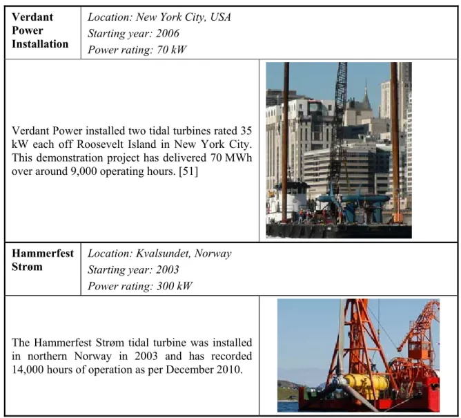
Table 2.1: Examples of grid-connected pilot wave power plants... 56 

Table 2.2: Examples of grid-connected pilot tidal current power plants... 58 

Table 2.3: Selected future grid-connected sites/projects ... 59 

Table 2.4: Response means to power dispatch requests ... 61 

Table 2.5: Capacity factors for some pilot power plants ... 62 

Table 2.6: Typical voltage levels for offshore marine energy applications [64] ... 64 

Table 2.7: Comparison of the different integration configurations [64] ... 67 

Table 2.8: Model types versus analysis type [75]. ... 77 

Table 2.9: Comparison of basic types of compensators [85] ... 80 

Table 3.1: Subsea cables lengths ... 107 

Table 3.2: Power variance ... 115 

Table 3.3: Period of the sinusoidal terms ... 123 

Table 3.4: Amplitude sets for the simulations ... 123 

Table 3.5: Phase shifts ... 124 

Table 3.6: Amplitudes and periods of the sinusoidal terms ... 126 

Table 3.7: Random phase shifts ... 126 

Table 3.8: Summary of summer and winter powerflow base cases (year 2019) ... 138 

Table 3.9: Northwest area interchange summary ... 139 

Table 3.10: Northwest Balancing Authority area loads and resources ... 139 

Table 3.12: Transfer description and sink system plants (units) ... 146 

Table 3.13: Typical relay and circuit breaker interrupting times ... 148 

Table 3.14: POI capacities for added new wave power ... 150 

Table 3.15: Power flow summaries of the combined base cases... 156 

Table 3.16: New renewable generation interconnection ... 159 

Table 3.17: Number of applied contingencies to the four cases in various types of studies ... 160 

Table 3.18: Maximum overloads for 2017 light load case with 700 MW ocean renewable generation ... 161 

Table 3.19: Load models for dynamic simulations ... 162 

Table 3.20: Relevant inter-area mode for the worst contingency before and after renewable resources ... 162 

A

CRONYMS

AC Alternating Current

AGC Automatic Generation Control

ATC Available Transmission Capacity

DC Direct Current

DFIG Doubly Fed Induction Generator

DG Distributed Generation

DSO Distribution System Operator

FACTS Flexible AC Transmission System

FRT Fault Ride-Through

GC Grid Codes

HV High Voltage

HVAC High Voltage Alternating Current

HVDC High Voltage Direct Current

IGBT Insulated Gate Bipolar Transistors

LCC Line Commutated Converter

MPPT Maximum Power Point Tracking

MSC Mechanically Switched Shunt Capacitor

MV Medium Voltage

NIA Non Integrated Area

ODE Ordinary Differential Equation

PCC Point of Common Coupling

PHEV Plug-in Hybrid Electric Vehicle

PM Permanent Magnet

POI Point of Interconnection

PSAT Powerflow and Short circuit Analysis Tool

PSS Power System Stabilisers

PTO Power Take Off

PWM Pulse Width Modulation

SC Squirrel Cage Generator

SG Static Gen

SPS Special Protection System

SSAT Small Signal Assessment Tool

STATCOM Static Synchronous Compensator

SVC Static VAR Compensator

TCR Thyristor Controlled Reactor

THD Total Harmonic Distortion

TSAT Transient Security Assessment Tool

TSC Thyristor Switched Capacitor

TSO Transmission System Operator

VAR Volt-Ampere Reactive

VSAT Voltage Security Assessment Tool

VSC Voltage Source Converter

WEC Wave Energy Converter

1 I

NTRODUCTION

1.1 BACKGROUND

Renewable energy from ocean wave and tidal current resources is an emerging resource option. Potential contribution of this energy resource towards electricity production and for other utilisations is being examined by various organisations in more than 25 countries. Several countries have embarked on research, demonstration and commercial operations to harness wave and tidal current energy resources. To provide a forum for information exchange related to integration of wave and tidal current energy into electrical systems, the International Energy Agency’s Implementing Agreement on Ocean Energy Systems (OES-IA) (www.iea-oceans.org) initiated a task-shared and cost-shared collaborative program in 2007, called Annex III. Task activities through this Annex were carried out in three work packages. This report presents the work performed in Work Package 3. The report also presents some earlier work carried out through this Annex and reported in the following three OES-IA documents:

 Potential opportunities and differences associated with integration of ocean wave

and ocean current energy plants in comparison to wind energy. OES-IA Document No: T0311 [1].

 Key features and identification of needed improvements to existing interconnection

guidelines for facilitating integration of ocean energy pilot projects. OES-IA Document No: T0312 [2].

 Dynamic characteristics of wave and tidal energy converters and a recommended

structure for development of a generic model for grid connection. OES-IA Document No: T0321 [3].

1.2 SCOPE

The variability of wave and tidal current resources as well as present generation characteristics of the wave and tidal current conversion processes are discussed in the following sub-sections of this first section. This section also presents the meaning of grid integration, defines various terms and discusses important grid integration issues (e.g., power quality, active and reactive power, etc.). Finally, grid codes are briefly discussed. Section 2 describes how various potential grid integration issues can be managed considering several factors, including deployment site, conversion systems, layout of devices and system control.

Sub-sections 3.1 and 3.2 show case studies illustrating integration of a wave energy plant into a typical distribution grid, whereas sub-sections 3.3 and 3.4 present case studies illustrating integration of aggregate wave energy and tidal current power plants into a larger power system at transmission levels.

Section 4 of the report presents some observations from this work and recommendations for future collaboration.

1.3 VARIABILITY AND INTERMITTENCY OF WAVE AND TIDAL

CURRENT RESOURCES

Renewable energy systems convert the energy flux from natural sources into useful forms. Therefore, the stochastic and periodic nature of various environmental elements affects the operation, output and availability of such energy converters. The frequency variation of the power produced from the renewable resources depends especially on the variability of the resources. The conversion principle and the mechanism employed can help smoothing this variation [4]. Table 1-1 shows the timescale of natural cycle of renewable energy

processes.

Table 1.1: Timescale of natural cycle of renewable energy processes [4]

Historically, resource intermittency and variability have been considered as the main obstacle to integration of many renewable energy sources. The key aspects in this regard are [1]:

 Lack of dispatchability: In the absence of sufficient prior knowledge (predictions

1 to 40 hours before) on how much generation can be realised from a time-varying generating source and what timeframe of operation can be ensured, the system operators find such variable sources difficult to synchronise with present or predicted load demand.

 Stress on the electrical grid: As the operation of many renewable energy systems

directly depends upon the variations in environmental conditions, a sudden increase in output or an outage from one or more of the surrounding generators may cause the neighbouring grid to reach its threshold of continuous operation. In addition, effects of flicker, harmonics and thermal overload may introduce various operational challenges.

 High penetration effects: With a minimal level of renewable energy integration into

the existing bulk power system, time variations are buried in the overall load generation mix. However, with higher penetration of such generating sources, occasional mismatch between existing load demand and generation level may cause the system to migrate from its equilibrium condition. In some European and North American countries, high penetration of wind energy is a major topic of interest.

Regarding tidal resources, the main characteristic is the predictability. In a tidal farm, the power production can be accurately forecasted. This is a big advantage compared to other renewable resources because the influence of the farm on the grid can be estimated. In economic terms, knowing the efficiency of the current tidal energy converters, the benefits can be estimated with a reasonable margin of error. However, the large variability of the tidal resource will pose challenges to the power systems.

The gravitational and rotational forces between the earth, moon and sun that cause water on the earth’s surface to move in different directions drive tides. The moon is the main cause of the existence of tides; however, the relative influence of the sun and moon varies over the course of a year. This results in variations in the tide height on a number of time scales [5].

 Daily Tides: the change in tide height that occurs each day is the most readily

observable tidal pattern. In many locations around the world, these tides occur on a semi-diurnal basis – roughly two high tides and two low tides each day. Local bathymetry and coastal geography will influence the tidal patterns of individual locations. Some locations may experience only one tide per day (diurnal), or show a mixture of the two depending on the spring-neap tide cycle. The timing of high and low tides is affected by location, particularly in areas where water flow is restricted.

 Spring and Neap Tides: The relative position of the moon and sun in relation to each

other has a significant effect on the daily tidal range.

Tidal currents occur when the tide forces water movement, particularly if that water is constrained by headlands, islands or channels. As tidal currents are a direct result of the action of tides, the pattern of variation is controlled by the pattern of tides.

Wave energy resources, however, depend largely on wind. Wind speed, duration of wind blow and fetch define the amount of energy transferred. Wave energy is subject to cyclic fluctuation dominated by wave periods and wave heights. Power levels vary both on a daily and monthly basis, with seasonal variations being less in more temperate zones. Power levels also vary on a wave-to-wave and wave group basis. A sea-state lasts around 10 to 20 minutes, so variation can be visible on a basis of minutes.

Taking into account wave and tidal current resource characteristics, the lack of dispatchability is not a main problem as both resources are more predictable than other renewable resources, such as wind. In the case of wave and tidal resources, significant variations are mostly limited between hourly and seasonal variations. Nevertheless, in the case of wave energy converters, stress on the electrical grid and high penetration effects may be serious obstacles due to the effect of wave by wave variability in the regulation time domain (seconds).

The Irish meteorological institute states, “The wave model outputs include hourly predictions of significant wave height and direction, mean wave period, peak period, significant height, direction and mean period of primary swell and sea/wind waves; and six-hourly outputs of the wave energy spectra. Waves can be forecast up to two days ahead on the Irish model and up to six days ahead on the European global model.” (http://www.met.ie/marine/marine_forecast.asp).

Waves can be forecasted, but not on the long term (e.g., precisely with significant height, mean period, etc. a week ahead). Existing global and local forecasting models needs to be refined and optimised to match the accuracy requirements demanded by grid operators for the integration of wave energy into the energy mix.

In spite of being highly variable and difficult to predict, wind energy has secured its place alongside other conventional energy sources. The key lessons learned from this technology include:

 The aggregation of wind generation reduces output fluctuations resulting from

resource variations. Aggregation also reduces prediction error.

 Improved forecasting methods allow greater penetration of wind power into the grid.  In order to maintain system stability and to supply the load demand, at higher

penetration levels ( >15% of energy) sufficient reserve capacity may be needed.

 Expansion and reinforcement of transmission and distribution grids plays a key role

in allowing higher levels of wind power integration into the grid.

 Newer technologies and management strategies support the grid and have paved the

path for fast growth of wind power.

Wave and tidal current generation schemes will undoubtedly require similar arrangements in order to be integrated into an electric grid. The good news is large scale wind may inadvertently lead in the management of wave and tidal current resources by forcing utilities to develop operational approaches to manage their variability. Solar energy in established markets may offer a model for the integration of wave and tidal current resources in the regulation time domain where impacts are likely to occur. Tracking the integration of wind and solar in established markets may offer solutions with the impacts of these variable ocean renewables.

Capitalising on the commonly perceived notion that wave and tidal resources are more predictable, development of reliable, effective and accurate forecasting methods will have multi-dimensional effects, such as:

 Resource assessment and prediction of wave/tidal plant output for feasibility/cost

studies.

 Becoming competitive to dispatchable generation units and providing ancillary

services.

 Avoiding scheduling penalties and contributing to reliability enhancement.

In brief, the effects of resource variability can be reduced by accommodating one or more of the following schemes:

 Resource forecasting.

 Intra- and inter-site smoothing.

 Generation and load mix (balancing area management).  Storage (i.e. large hydro, pumped hydro, battery storage).  Load forecasting and demand side management.

 Generation/load flexibility offering could be most cost effective solution. This is the

1.4 PRESENT GENERATION CHARACTERISTICS OF WAVE AND

TIDAL CURRENT CONVERSION PROCESSES

A brief look at the ocean energy conversion schemes reveals that most of the tidal current energy conversion devices are analogous to wind turbines and these units mostly utilise designs, concepts and equipment that originated in the wind industry (Figure 1.1). In sharp contrast to wind and tidal turbines, wave energy converters operate on diverse principles and may require cascaded conversion mechanisms.

Figure 1.1: Ocean Energy Conversion Systems (Tidal and Wave) [1].

Even though tidal turbines can be viewed through established terms and definitions of the wind energy literature, studying wave energy devices poses a unique challenge. Different systems operate on different methods of wave-device interaction (such as heave, pitch or surge) and may need pneumatic, hydraulic or mechanical power take-off (PTO) stages. As in any efficiency calculation, addition of a second energy conversion feature, whether electrical or mechanical, may introduce efficiency degradation since losses are multiplicative in nature (this includes energy storage if included in the design, either at the plant or at the grid level). Wave and tidal technologies with a simple mechanical to electrical conversion are likely to dominate more complicated designs for this reason. Power electronics will likely enable wave and tidal resources to offer transmission support, which may provide a secondary value stream to make respective projects more economic. In addition, placement of these devices (distance from shore, depth from surface and orientation with respect to the wave-front) and subtle structural aspects (resonance, directionality, etc.,) may blur the definition of operating principles. While the front-end stages may have significant diversity in design, the final stages of conversion (i.e. electric machines and equipment) are generally very similar for both wind and ocean (tidal or

wave) power plants, though reactive support for wave conversion will continue to be an issue for weak buses without energy storage.

Tidal current energy systems convert the kinetic energy of a water flow into the motion of a mechanical system, which can then drive a generator. Regarding the type of the rotor, there are two different concepts, axial flow rotors and cross flow rotors. Cross flow rotors are characterised by having the axis of rotation perpendicular to the flow [6].

Most of the devices can be characterised as belonging to one of four types:

 Horizontal axis systems such as SeaGen [7], which has been installed at Strangford

Lough, Northern Ireland.

 Vertical axis systems such as the ENERMAR [8] device, which was tested in the

Strait of Messina between Sicily and the Italian mainland.

 Reciprocating hydrofoil systems such as Stingray [9], which has been tested in Yell

Sound in Shetland, which lies to the north of Scotland and Orkney.

 Venturi effect systems such as the Lunar Energy device [10], which uses pressure

changes induced by flow constriction to drive a secondary hydraulic or pneumatic turbine.

Wave and tidal energy devices currently make use of a very wide range of technologies for primary energy conversion. All of the concepts aiming at generating electricity must include an electrical generator in the design, generally driven by an intermediate mover, but in some cases directly driven by the motion of the device itself. The different PTO systems can be classified in seven different concepts:

 Air turbines

 Hydraulic turbines contained in a closed circuit of pressurised oil

 Direct drive (linear generator using moving or stationary coils and moving or

stationary permanent magnets)

 Low head water turbine  Water pump

 Hydraulic turbine contained in an open circuit of sea water

Most of wave energy converters at an advanced stage of development have considered hydraulic systems for energy conversion. The motion of the device is in this case transferred to a hydraulic motor, which runs a conventional rotary generator. Pelamis [11], for instance, runs a hydraulic motor coupled with an asynchronous generator spinning at 1500 rpm.

Other technologies, mainly heaving point-absorbers, convert the power through directly driven generators, translating at a variable velocity and therefore generating output at variable frequency.

Tidal devices, especially horizontal (parallel to flow) axis turbines, present more similarities with the conventional wind turbine conversion mechanisms, with a gearbox interfacing between the shaft and the rotor of an electrical generator.

The step of electrical conversion consists of a generator and power electronics to adapt the energy generated to the grid, at the point where the energy converter is connected. The choice of the type of generator will influence the rating level of power electronics required as well as the type of grid connection interface and control. A brief summary of the existing technologies applicable to ocean energy devices is given below [12]:

 Synchronous Machines: The field source is provided by DC electromagnets, usually

located on the rotor. Current in field coils can be adjusted to load, so that the power factor can be kept close to unity or within prescribed values. An external electric power source is needed to feed rotating DC coils.

 Permanent Magnet Synchronous Machines: Instead of electromagnets, rare-earth

(usually neodymium [NdFeB]) permanent magnets are implemented. In machines rated up to a few MW, permanent magnets allow for remarkable improvements in terms of power density and design/manufacturing simplicity (no DC power source required).

 Variable Reluctance Synchronous Machines: Magnets are replaced by toothed-iron

in the rotor, magnetised by the armature field windings. These machines are low-cost, have a simple design and a remarkably low power density. Variable-speed Synchronous Machines require fully-rated (MVA) power converters.

 Induction Generators: There is no autonomous field source. Rotor circuits hold

low-frequency AC currents induced by armature field coils in the stator. No-load voltage is therefore zero and the power factor is always lower than unity. Air-gap length is determinant for performance (the smaller the better). Squirrel-cage machines have solid bars of conducting material; rotor-wound machines have windings.

 Doubly-Fed Induction Generators (DFIG): The frequency of the rotor currents is

controlled by a power converter. Since the power electronics converter is rated for only a fraction of maximum machine power capability, it represents a very

convenient solution for applications where the speed is varied within limits (e.g., 30%) of the rated value.

 Linear Generators: A typical wave energy converter with a linear generator consists

of a buoy, floating on the surface of the ocean, connected with a cable to the rotor. The piston, in turn, is moving in a coil where electricity is induced. The tension in the cable is maintained with a spring attached at the bottom of the piston.

Induction machines are cheap and reliable, but encumbrance and efficiency may make them unfit for certain applications. Low speed direct drive energy conversion, for example, requires generators with torque/force density as high as possible. This is the case of linear generators for wave power, where the speed rarely exceeds one to two metres per second. Literature recommends permanent magnet technology for this class of electric machines.

1.5 POWER SYSTEM STABILITY AND CONTROL

The main task of an electric power system is to convert energy from one of the available primary sources to electrical form and to transport it to the points of consumption. Energy is seldom consumed in the electrical form; the advantage of the electrical form of the energy is that it can be transported and controlled with relative ease and with a high degree of efficiency and reliability. A properly designed and operated power system should meet the following fundamental requirements [13].

 The system must be able to meet the continuously varying load demand for active

and reactive power. Since electricity cannot be conveniently stored in sufficient quantities, adequate spinning reserves of active and reactive power should be maintained and appropriately controlled at all times.

 The system should supply energy at minimum cost and with minimum ecological

impact.

 The quality of power supply must meet certain minimum standards with regard to

the following factors:

▬ Constancy of frequency (frequency stability). ▬ Constancy of voltage (voltage stability). ▬ Level of reliability.

In Figure 1.2 various subsystems and associated controls are depicted. In this structure, there are controllers operating directly on individual system elements. In a generating unit, these consist of prime mover controls and excitation controls.

The primary purpose of the system-generation control is to balance the total system generation against system load and losses so that the desired frequency and power interchange with neighbouring systems (tie flows) are maintained.

The transmission controls include power and voltage control devices, such as SVC, synchronous condensers, switched capacitors and reactors, tap-changing transformers, phase-shifting transformers and HVDC controls.

The controls described in Figure 1.2 not only contribute to the satisfactory operation of the power system but also have a profound effect on the dynamic performance of the power system, and on its ability to cope with disturbances.

Major system failures are usually brought about by a combination of circumstances that stress the grid beyond its capability. Severe natural disturbances (such as a tornado, severe storm or freezing rain), equipment malfunction, human error and inadequate design combine to weaken the power system and eventually lead to its breakdown [13].

Figure 1.2: Subsystems of a power system and associated controls [13]

The impact of time varying generation sources, such as wind, wave or tidal, can be studied through three time domains (Figure 1.3):

 Regulation: Short-term (seconds-minutes) balance management using methods such

as automatic generation control (AGC).

 Load-Following: Mid-term (minutes-hours) arrangement to follow the load

variations, such as morning peak-load and evening light-load conditions.

 Scheduling and Unit Commitment: Securing sufficient generation in advance (hours

Figure 1.3: Load balance and scheduling [1].

Before introducing aspects regarding power quality, it is of a very high importance to understand how the power system works and guarantee quality energy supply at any point on the grid. The following sections of this chapter explain how the power system manages to assure reliable service, i.e., remain intact and be capable to withstanding a wide variety of disturbances [13].

1.5.1 Power System Control

A properly designed and operated power system should be able to meet the continually changing load demand for active and reactive power. Since electricity cannot be conveniently stored in sufficient quantities, adequate spinning reserves of active and reactive power should be maintained and appropriately controlled at all times.

At the same time, the system should supply energy at minimum cost and be able to guarantee the quality of power supply. The power supply must follow standards of quality which include the following factors:

 Constancy of frequency (frequency stability).  Constancy of voltage (voltage stability).  Level of reliability.

Operating States of a Power System and Control Strategies

Regarding power system security and the design of appropriate control systems, it is useful to take into account the following figure in order to classify system operating conditions (Figure 1.4):

Figure 1.4: Power system operating states [13]

 Normal state: The system variables are within the normal range and there is no

overloaded equipment.

 Alert state: The security level falls below the normal range or the possibility of a

disturbance increases because of adverse weather conditions. In this state, all the system variables are still within acceptable range and all constraints. To restore the system to the normal state, preventive actions can be taken such as generation shifting (i.e., security dispatch) or increased reserve.

 Emergency state: When the system is in the “alert state” and a severe disturbance

occurs. Voltages at many buses are low and/or equipment loadings exceed short-term emergency ratings. The system is still intact and may be restored to the alert state by the initiating of emergency control action:

▬ Fault cleaning ▬ Excitation control ▬ Fast-valving ▬ Generation tripping ▬ Generation run-back ▬ HVDC modulation ▬ Load curtailment

 In extremis state: If the above-listed measures are not applied or are ineffective, the

result is cascading outages and possibly a shut-down of a major portion of the system. Control actions, such as load shedding and controlled system separation, are aimed at saving as much of the system as possible from a widespread blackout.

 Restorative state: Control action reconnects all the facilities and restores system

load. Depending on the system conditions, the system goes from this state to alert state or normal state.

1.5.2 Power System Inertia

System inertia is the capacity of the power system to oppose changes in frequency [14]. Physically, it is loosely defined by the mass of all the synchronous rotating generators and motors connected to the system. In a power system with high inertia, frequency will fall slowly during a system disturbance, such as a generator tripping off line. On the other hand, in a power system with low inertia, frequency will fall faster during a loss of generation.

Although system inertia does not provide frequency control per se, it does influence in the time it takes for the frequency to recover from a given disturbance or loss of generation. Thus, higher system inertia is better than lower system inertia because it will provide more time for governors to respond to the drop in frequency [15]. Replacing conventional synchronous generators by a large number of DFIG or full converter synchronous generators will reduce the angular momentum of the system. Active power control with an additional loop is needed to tackle this problem.

1.5.3 Power System Stability Problem

Power system stability can be defined as the property of a power system that enables it to remain in a state of operating equilibrium under normal operating conditions and to regain an acceptable state of equilibrium after being subjected to a disturbance. In the evaluation of stability, the behaviour of the power system is analysed when subjected to a transient disturbance.

The following classification of stability into various categories [16] helps provide the understanding of stability problems (Figure 1.5).

 Rotor angle stability: The ability of the interconnected synchronous machines of a

power system to remain in synchronism. This stability problem involves the study of the electromechanical oscillations inherent in power system.

 Small-signal stability: The ability of the power system to maintain synchronism

under small disturbances due to small variations in loads and generation. These disturbances are considered small enough for linearisation of system equations.

 Transient stability: The ability of the power system to maintain synchronism when

subjected to a severe transient disturbance. Stability depends both on the initial conditions and on the severity of the disturbance. The resulting system response involves large excursions of generator rotor angles and is influenced by a nonlinear power-angle relationship.

 Voltage stability: The ability of a power system to maintain steady state acceptable

voltages at all buses in the system under normal operating conditions and after being subjected to a disturbance. When the system condition causes a progressive and uncontrollable drop in voltage, the system enters in to a state of voltage instability. The incapability of the power system to meet the demand for reactive power is the main factor causing voltage instability. Another reason for the progressive drop in bus voltage can be associated with rotor angle going out of step due to the nonlinear power-angle relationship. Even though voltage instability is in essence a local phenomenon, its consequences may have a widespread impact.

 Large-disturbance voltage stability: This form of stability is involved with a

system’s ability to control voltages following large disturbances such as system faults, loss of generation or circuit contingences. This is determined by the system-load characteristics and the interaction of both continuous and discrete controls and protection schemes. Determination of large-disturbance stability requires the

examination of the nonlinear dynamic performance of a system over a period of time (from a few seconds to tens of minutes).

 Small-disturbance voltage stability: This form of stability is involved with a

system’s ability to control voltages following small perturbations, such as incremental changes in system load. This form of stability is determined by the characteristics of the load, both continuous and discrete load changes (controls) at a given instant of time. Static analysis can be used to carry out small-disturbance voltage stability analysis because the basic processes contributing to small-disturbance voltage instability are of a steady state.

 Voltage collapse: This form of stability it is more complex than simple voltage

instability and is usually the result of a sequence of events coupled with voltage instability leading to a low-voltage profile in a significant part of the power system. Usually this is due to the inability of the power system to supply the full amount of reactive power required and consumed by long transmission lines, such as

attempting to carry loads exceeding the Available Transmission Capacity (ATC) of the lines themselves.

 Mid-term and long-term stability problems: These stability problems are associated

with inadequacies in equipment responses, poor coordination of control and protection equipment, or insufficient active/reactive power reserves (i.e., with problems associated with the dynamic response of the power system to severe disturbances). In mid-term stability studies, the focus is on synchronising power oscillations between machines; whereas in the case of long-term stability studies, the focus is on the slower and longer-duration phenomena that accompany large-scale system disturbances and the resulting large, sustained mismatches between generation and consumption of active and reactive power.

1.5.4 Classification of Stability

Instability of the power systems can take different forms and can be influenced by a wide range of factors. Analysis of stability problems, identification of essential factors that contribute to instability, and the formation of methods of improving stable operation are greatly facilitated by classification of stability into appropriate categories. These are based on the following considerations [16]:

 The physical nature of the resulting instability.  The size of the disturbance considered.

 The devices, processes and time span that must be taken into consideration in order

to determine stability.

35

Power System Stability

Angle Stability Voltage Stability

Small-Signal

Stability Transient Stability

Non-oscillatory Instability Oscillatory Instability Local Plant Modes Interarea Modes Torsional Modes Control Modes Long-term Stability* Mid-term Stability* Large-Distrubance Voltage Stability Small-Distrubance Voltage Stability

- Ability to remain in operating equilibrium - Equilibrium between opposing forces

- Ability to maintain synchronism - Torque balance of synchronous machines

- Large distrubance - First-swing aperiodic drift - Study perod up to 10s

- Insufficient synchronizing torque - Insufficient damping torque - Unstable control action

- Severe upsets; large voltage and frequency excursions - Fast and slow dynamics - Study period to several min.

- Uniform system frequency - Slow dynamics - Study period to tens of min.

- Large disturbance - Switching events - Dynamics of UTLC, loads

- Coordination of protections and controls

- Steady-state P/Q – V relations - Stability margins, Q reserve

* With availability of improved analytical techiques providing unified approach for analysis of fast and slow dynamics, distinction between mid-term and long-term stability has become less significant.

1.6 POWER QUALITY

To assure that the energy is transported and controlled with relative ease and with a high degree of efficiency and reliability, a specific level of power quality, must be guaranteed. In this report, the following definitions are considered [17]:

 Voltage quality is concerned with deviations of the voltage from the ideal voltage. The

ideal voltage is a single-frequency sine wave of constant amplitude and frequency.

 Current quality is the complementary term to voltage quality. The ideal current is again

a single-frequency sine wave of constant amplitude and frequency, with the additional requirement that the current sine wave is in phase with the voltage sine wave.

 Quality of supply is a combination of voltage quality and the non-technical aspects of

the interaction from the power grid to its customers.

 Quality of consumption is the complementary term to quality of supply.

Power quality is the combination of voltage quality and current quality and is an issue to be

managed locally at the point of connection (POC). All definitions given above apply to the interface between the grid (electric utility) and the customer. The term power quality is certainly not restricted to the interaction between the power grid and end-user equipment. Depending on the way a characteristic of voltage or current is measured, power quality disturbances can be defined as variations or events.

 Variations are small deviations of voltage or current characteristics from their nominal

or ideal value. Variations are measured at any moment in time.

 Events are larger deviations that only occur occasionally. Events are disturbances that

start and end with a threshold crossing.

The chief difference between variations and events is that variations can be measured at any moment in time whereas events require waiting for a voltage or current characteristic to exceed a pre-defined threshold. As the setting of a threshold is always somewhat arbitrary, there is no clear border between variations and events. Regardless, the difference between them remains useful and is analyzed (implicitly or explicitly) in almost every relevant study. With a limited number of large power stations and an adequate transmission and distribution system, the electrical power system can distribute electrical power with a high power quality, with a fixed frequency, at a fixed voltage level and in a reliable way. The power is then transmitted via high voltage transmission lines and distributed via medium and low voltage distribution systems with good protection systems. The protection systems are sized based on the power flow from the power stations via the transmission lines and the distribution system to the customers (Figure 1.6).

In the classical definition of the power system, the customers are traditionally referred to as loads. However, due to changes in these traditional loads (i.e., becoming more nonlinear) a modern model of power system has developed. Two developments can be highlighted: 1) the deregulation of the electricity industry; and 2) the increased number of smaller units connected at lower voltage levels. Because of this, the power system can no longer be seen as one entity, but as an electricity grid with customers. This new model is shown in Figure 1.7.

Figure 1.7: Modern model of power system [17].

To maintain a fixed voltage and frequency in a reliable way becomes more difficult as the contributions from distributed generation increases, especially in the case of variable renewable energy sources.

This is because these systems:

 Do not always contribute to voltage control, as they often do not vary reactive power

output (especially older systems);

 Can disturb frequency control and cause voltage variations, due to the variability of the

delivery of active power.

 Under voltage disturbances, they may disconnect and lead to significant loss of

generation and thus disturb the power balance.

 May affect the protection system, when they connect to the distribution system and

may change the power flow direction.

For wind energy, these aspects are being investigated and several problems have been solved [18]. Because of the similarities between wind and other renewable energy sources, wave and tidal energy can profit from this knowledge.

A set of possible grid impact issues can be broadly linked with wave and tidal current turbine farm power plant size and area of impact as indicated in Figure 1.8. While many of these factors are interrelated and cannot be viewed separately (such as reactive power and voltage stability), this approach differentiates between the effects of a small project against large future projects and development initiatives [1].

Energy buffering for wave energy converters may represent a serious issue since the raw power produced by a single unit may cause voltage variations at the connection node depending on the grid strength. Due to wave grouping in a given sea state, a large number of devices opportunely deployed can reduce the short-term variations of the output power.

Figure 1.8: Possible grid impact issues pertaining to ocean energy systems [1].

1.6.1 Local Impact and Power Quality Issues

The impact of wave and tidal farms depends on the strength of the grid. A weaker grid will suffer larger voltage variations at the connection point than a strong one; this is because of the impedance of the grid. In a weak grid, this impedance is high and in this scenario a small amount of generation can greatly affect the steady-state voltage. Taking into account that many wave and tidal energy converters and farms will be connected to the distribution system close to shore (i.e., to grids with high impedance), many grid integration aspects should be analysed to assess suitable and secure operation both of the wave farm and of the grid.

A single ocean energy converter connected to the distribution system close to shore does not have a significant impact on entire grid. However, there may be some local effects in the distribution system where the ocean energy converter is connected, such as:

 Voltage variations  Harmonics  Flicker

 Performance during grid disturbances faults

Power electronic converters produce harmonics, but state-of-the-art filtering will usually keep these below a prescribed value. It has to be noted that the most modern electronic converters (based on insulated gate bipolar transistor [IGBT] thyristers) produce harmonics at their pulse wave modulation (PWM) frequency and at some multiple frequencies of the commutation frequency. All these frequencies are between 2 kHz and 9 kHz. Some effects were detected on loads but further studies are still needed in order to examine this issue in detail.