Design of a quasi-passive parallel leg exoskeleton to augment load carrying for walking

Design of a Quasi-Passive Parallel Leg Exoskeleton to

Augment Load Carrying for Walking

by

Andrew Valiente

B.S., LeToumeau University (2003)

Submitted to the Department of Mechanical Engineering in partial fulfillment of the requirements for the degree of

Master's of Science

at the

MASSACHUSETTS INSTITUTE OF TECHNOLOGY August 2005

C Massachusetts Institute of Technology 2005. All rights reserved.

Author ... rr.a 7IA

Departme/f Mechanical Engineering August 5 2005

C ertified by... ...

Hugh Herr Assistant Professor of Media Arts and Sciences, MIT Thesis Supervisor

C e r t i f i e d b y . . . .......

me ,!::sl!]I to Banco Professor of Mechanical Engineering Thesis Supervisor

Accepted by ... ... ...

Professor Lallit Anand Chairman, Departmental Committee on Graduate Students

MASSACHUSETTS INSTITUTE OF TECHNOLOGY

APR 1

3

2006

LIBRARIES

Design of a Quasi-Passive Parallel Leg Exoskeleton to Augment

Load Carrying for Walking

by

Andrew Valiente

Submitted to the Department of Mechanical Engineering on August 5, 2005, in partial fulfillment of the

requirements for the degree of Masters of Science

Abstract

Biomechanical experiments suggest that it may be possible to build a leg exoskeleton to reduce the metabolic cost of walking while carrying a load. A quasi-passive, leg exoskeleton is presented that is designed to assist the human in carrying a 75 lb payload. The exoskeleton structure runs parallel to the legs, transferring payload forces to the ground. In an attempt to make the exoskeleton more efficient, passive hip and ankle springs are employed to store and release energy throughout the gait cycle. To reduce knee muscular effort, a variable damper is implemented at the knee to support body weight throughout early stance. In this thesis, I hypothesize that a quasi-passive leg exoskeleton of this design will improve metabolic walking economy for carrying a 751b backpack compared with a leg exoskeleton without any elastic energy storage or variable-damping capability. I further anticipate that the quasi-passive leg exoskeleton will improve walking economy for carrying a 751b backpack compared with unassisted loaded walking. To test these hypotheses, the rate of oxygen consumption is measured on one human test participant walking on a level surface at a self-selected speed. Pilot experimental data show that the quasi-passive exoskeleton increases the metabolic cost of carrying a 751b backpack by 39% compared to carrying 75 lbs without an exoskeleton. When the variable-damper knees are replaced by simple pin joints, the metabolic cost relative to unassisted load carrying decreases to 34%, suggesting that the dampening advantages of the damper knees did not compensate for their added mass. When the springs are removed from the aforementioned pin knee exoskeleton, the metabolic cost relative to unassisted load carrying increased to 83%. These results indicate that the implementation of springs is beneficial in exoskeleton design.

Thesis Supervisors: Hugh Herr and Ernesto Blanco

Title: Assistant Professor of Media Arts and Sciences, MIT Title: Professor of Mechanical Engineering, MIT

Acknowledgments

I would like to first and foremost thank Jesus Christ my Lord and Savior for endowing me with a talent for engineering, and for the myriad of past blessings that he has given me.

I would like to thank my advisor Professor Hugh Herr for making the Biomechatronics group at the Media Lab an incredible place to work and for his insight in biomechanics. Thanks to my thesis reader, Ernesto Blanco, for his encouragement and insight in mechanics.

Thanks to my coworkers at Biomechatronics Group: Dan Paluska, Dr. Ken Pasch, Conor Walsh, William Grand, and Chi Won for their support and collaboration in building exoskeletons. I extend appreciation to Dan Paluska for his encouragement, for answering my endless questions and for taking time away from his thesis to help me with my research.

I would like to thank Spaulding Rehabilitation Hospital for lending us V0 2 equipment

to conduct metabolic tests.

I would like to thank the Bill and Melinda Gates foundation for their fellowship that enabled me to study at MIT.

This research was done under Defense Advanced Research Projects Agency (DARPA) contract #NBCHC040122, 'Leg Orthoses for Locomotory Endurance Amplification'.

Table of Contents

A bstract ...

3

A cknow ledgm ents...

5

C hapter 1

Introduction...

13

1.1 Antigravity Experim ents ... 13

1.2 Past work... 14

1.3 Biom echatronics Quasi-Passive Exoskeleton ... 18

1.4 Thesis Overview ... 20

1.5 Com pleted Exoskeleton ... 21

1.6 Definitions... 24

Chapter 2 Passive Element Optimization... 25

2.1 Introduction... 25

2.2 M otivation... 26

2.3 Biom echanics Data... 28

2.3.1 Applying Backpack Data for Exoskeleton Analysis ... 28

2.3.2 Sum m ary of Data... 30

2.4 Analytical M ethods ... 34

2.4.1 Optim izing the Hip and Ankle Springs ... 34

2.4.2 Optimization Algorithm for a Knee Damper ... 36

2.4.3 Hip Power... 37

2.4.4 Knee Power ... 38

2.4.5 Ankle Power ... 40

2.5 Analytical Results ... 41

2.5.1 Sum m ary of Results ... 41

2.5.2 Hip Power... 44

2.5.3 Knee Power ... 46

2.5.4 Ankle Power ... 47

2.6 Lim itations and Future W ork ... 50

Chapter 3 M echanical Design ... 51

3.1 Introduction... 51

3.2 Force Transfer ... 51

3 .3 H ip ... 5 2 3.3.1 Hip Kinem atics... 52

3.3.2 Cam Design ... 54

3.3.3 Leg Extension Bearing Analysis ... 60

3.3.4 Abduction Bearing Implem entation ... 68

3.3.5 Hip abduction spring ... 68

3.3.6 Hip extension spring... 70

3.3.6.1 Energy Storage ... 70

3.3.6.2 Anti m om ent ... 71

3.4 Thigh ... 72

3.5 Knee ... 72

3.6 Ankle ... ₇₃

3.7 Sum m ary ... 74

Chapter 4 Experimental M ethods ... 75

4.1 Introduction ... 75

4.2 Study Participant ... 75

4.3 Quantifiable M etric ... 76

4.4 Experim ental Procedure ... 76

Chapter 5 Experimental Results...79

5.1 Quantitative Results ... 79

5.2 Qualitative Results ... 81

C hapter 6 Dc s... sion ... 83

6.1 Introduction... 83

6.2 Discussion of Experim ental Results ... 83

6.2.1 Comparison 1 ... 83 6.2.2 Com parison 2 ... 83 6.2.3 Com parison 3 ... 84 6.2.4 Com parison 4 ... 84 6.2.5 Com parison 5 ... 85 6.3 Design ... 85

6.3.1 Controllability of the Variable-Damping Knee ... 86

6.3.2 The carbon composite foot-ankle bi-directional constraint... 87

6.3.3 Flexion in hip harness ... 87

6.4 Sum m ary ... 88

C hapter 7 Future W ork ... 89

7.1 Introduction ... 89

7.2 Redesign... 89

7.2.1 Alignm ent... 89

7.2.2 Variable-Damping Knee... 89

7.2.3 Uni-directional Ankle Spring ... 90

7.2.4 Hip Harness ... 91

7.3 Exoskeleton Data Set ... 91

7.4 M easuring the Exoskeleton's Kinematic Efficiency ... 92

7.5 Adding Power... 93

C hapter 8 C onclusions... 95

B ibliography ... 97

A ppendix ... 101

A .1 N atick Army Lab Data [Harm an et al. (2000)] ... 103

Figures

Figure 1 Summary of metabolic experiments ... 14

Figure 2 Historic exoskeletons... 16

Figure 3 Present day exoskeletons... 18

Figure 4 Inverted pendulum motion model for walking [Farley et. al. (1998)]... 19

Figure 5 Distribution of exoskeleton mass ... 21

Figure 6 The author in all his glory -wearing the completed exoskeleton... 22

Figure 7 Exoskeleton architecture and major components ... 23

Figure 8 Body plane and axis definitions [Sutherland, et al. (1994)] ... 24

Figure 9 Negative and positive joint power during walking [Rab (1994)]... 27

Figure 10 Gait cycle for normal walking [Inman (1981)]... 30

Figure 11 Joint angles, natural and 47 kg backpack ... 31

Figure 12 Joint velocities, natural and 47 kg backpack ... 32

Figure 13 Joint torques, natural and 47 kg backpack... 33

Figure 14 Joint power, natural and 47 kg backpack... 33

Figure 15 Hip power [Harman et al. (2000)] ... 38

Figure 16 Knee power [Harman et al. (2000)]... 38

Figure 17 Ankle power [Harman et al. (2000)] ... 41

Figure 18 Residual joint powers ... 43

Figure 19 Residual hip power ... 44

Figure 20 Residual hip torque... 44

Figure 21 Hip spring energy... 45

Figure 22 H ip spring ... 45

Figure 23 Residual knee power... 46

Figure 24 Residual knee torque ... 47

Figure 25 Residual ankle power... 48

Figure 26 Graphical representation of ankle spring [Au (2005)]... 48

Figure 27 Residual ankle torque ... 49

Figure 28 Ankle spring energy... 49

Figure 29 A nkle Spring... 50

Figure 30 Human/exoskeleton interface ... 51

Figure 31 Backpack and hip harness... 52

Figure 32 Hip medial/lateral rotation and flexion/extension ... 53

Figure 33 Change in leg length during hip abduction... 54

Figure 34 Vector representation of exoskeleton and human leg kinematics ... 55

Figure 35 Cam profile described by 'r6' in Figure 34 ... 57

Figure 36 C am m echanism ... 57

Figure 37 Instant center of rotation for the exoskeleton leg ... 58

Figure 38 Virtual center of exoskeleton leg and the cam profile ... 59

Figure 39 Virtual exoskeleton hip joint center superimposed on biological hip center of a 50 percentile man [Tilley 1993]... 59

Figure 40 Exoskeleton leg diagram ... 60

Figure 41 Free body diagram of the cam roller... 61

Figure 42 Force balance of the cam roller ... 62

Figure 43 Force amplification on the roller. ... 63

Figure 44 Free body diagram of the full exoskeleton leg. ... 64

Figure 45 Free body diagram of the upper and lower parts of the exoskeleton leg ... 65

Figure 46 Free body diagram of the shaft and bearings... 66

Figure 47 Bearing reaction forces ... 67

Figure 48 Leg length vs hip abduction angle ... 67

Figure 49 Free body diagram of the harness ... 69

Figure 50: Abduction spring ... 70

Figure 51: Hip extension spring... 71

Figure 52: Backpack overturning moment... 72

Figure 53: Frontal view of thigh cuff... 72

Figure 54: Variable-damping knee... 73

Figure 55: Carbon-fiber foot-ankle ... 74

Figure 56 Bi-directional ankle action... 87

Figure 57 Uni-directional ankle action ... 91

Figure 58 College Park Tribute... 91

Figure 59 Average walking metabolic rate: 1084 mL/min ... 107

Figure 60 Average resting metabolic rate: 320 mL/min ... 107

Figure 61 Average walking metabolic rate: 1089 mL/min ... 108

Figure 62 Average resting metabolic rate: 336 mL/min ... 108

Figure 63 Average walking metabolic rate: 1046 mL/min ... 109

Figure 64 Average resting metabolic rate: 418 mL/min ... 109

Figure 65 Average walking metabolic rate: 817 mL/min ... 110

Figure 66 Average resting metabolic rate: 397 mL/min ... 110

Figure 67 Average walking metabolic rate: 807 mL/min ... 111

Figure 68 Average resting metabolic rate: 340 mL/min ... 111

Figure 69 Average walking metabolic rate: 658 mL/min ... 112

Tables

Table 1 H ypotheses stated... 20

Table 2 Summary of results from the passive element optimization... 25

Table 3 Summary of results from Bogert and Paluska/Herr ... 28

Table 4 Summary of data used for analysis ... 29

Table 5: Spring variables for residual energy minimization... 36

Table 6: Damper variables for residual energy minimization... 37

Table 7 Summary of positive/negative energy of joints ... 40

Table 8 Summary of passive elements implemented in the exoskeleton... 42

Table 9 Energy benefit due to passive elements ... 43

Table 10: Dimensions for the four bar linkage in Figure 34... 56

Table 11 Equations from the full exoskeleton leg free body diagram in Figure 44... 64

Table 12 Equations from upper exoskeleton leg free body diagram in Figure 45 ... 65

Table 13 Equations from shaft and bearings free body diagram in Figure 46 ... 66

Table 14: Thompson linear motion parts and specifications ... 68

Table 15 H ypotheses R estated ... 75

Table 16 Experimental Participants for studies done by MIT and Natick Army Labs ... 76

Table 17 Participant guidelines... 77

Table 18 Experim ental Procedure... 78

Table 19 Experimental metabolic results... 79

Table 20 Comparing exoskeleton configurations ... 80

Table 21 Com paring knee joints ... 80

Table 22 Comparing springs and no springs... 81

Table 23 Unloaded exoskeleton baseline... 81

Table 24 Incremental Cost ... 81

Chapter 1 Introduction

1.1 Antigravity Experiments

Exoskeletons can enhance human locomotory performance and can augment human strength, endurance, and speed. Exoskeletons have application for military and service personnel, as well as for patients with muscular impairments. Exoskeletons have the ability to traverse non-paved terrain accessing locations where wheeled vehicles cannot. Exoskeletons promise to allow people to run farther, jump higher, and bear larger loads while expending less energy.

Recent physiological studies suggest that it may be possible to build an orthotic exoskeleton to dramatically increase the locomotory endurance of service personnel. Simulated reduced gravity experiments have demonstrated that the metabolic cost of walking and running can be reduced by 33% and 75% respectively, if gravity is reduced by 75% [Jiping et al. (1991); Farley & McMahon (1992)]. These experiments have shown that if gravity is decreased by at least 50%, then a person can run at a lower metabolic rate than he could have walked. Furthermore, studies by [Griffen et al, (2003)] have shown that a 10% and 30% increase in body mass (BM) will increase the required metabolic energy of walking by 15% and 47% respectively. Studies by Gottschall and Kram, 2003 have shown that a 10% bodyweight forward assist will cause a 47% reduction in metabolic energy, while a 10% drag force will cause a corresponding 150% increase in metabolic cost.

The reduced gravity experiments suggest that the metabolic energy expended by an average 200 lb person bearing a 751b backpack (38% BM), will increase substantially. It can be reasoned that an exoskeleton placed in parallel to the human body can transmit the backpack forces to the ground relieving the human from supporting the load. Thus, it is reasoned that if an exoskeleton is designed correctly, a lower metabolic cost can be achieved for loaded walking. A summary of the metabolic studies is shown in Figure 1.

unweighting force

_vo

50% antigravity

25% reduction

Fodey & MCOohon, 1992

forward

assist force

10% OW assist 47% reduction

drag force

Gotischoll & Krom, 2003

10% BW impeding

_{addifonal mass}

150% Increase _{10% SM addition}

GolischoH & Kram, 2003 _{15% Increase}

Grffin et al, 2003

Figure 1 Summary of metabolic experiments.

Simulated antigravity experiments suggest that it may be possible to build an orthotic exoskeleton to augment human load carrying capabilities while reduce the metabolic cost of locomotion.

1.2

Past work

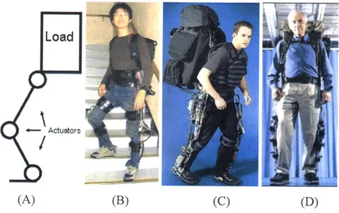
The idea of using exoskeletons to augment human locomotory performance dates back to 1890 when Nicholas Yagn conceptualized an apparatus for facilitating walking, running, and jumping [Yagn (1890)]. _{See Figure 2A. His device consisted of a large} bow spring that was interconnected between a hip belt and a foot attachment. The bow spring stores energy developed by the weight of the body and by the act of walking, running, or jumping. Yagn's bow spring design lacked a degree of freedom at the knee. Therefore, to achieve steady state running the user would hop from one leg to the other. Bending of the knee for normal walking and running would require storing prohibitive amounts energy in the bow spring. Yagn's apparatus was completely passive and human powered.

In 1969, the 'kinematic walker' was developed [Vukobratovid et al. (1990)]. See Figure 2B. Each leg of the 'kinematic walker' consisted of 2 degrees of freedom with an active joint at the hip and a passive joint at the ankle. The knee was locked straight and the hips were actuated via pneumatic pistons mounted on the waist. The resulting gait was of the 'sliding foot type'.

In 1970, the first active exoskeleton with 3 degrees of freedom per leg was developed [Vukobratovid et al. (1990)]. See Figure 2C. This exoskeleton, know as the 'partial

exoskeleton', introduced a degree of freedom at the knee. It employed 7 pneumatic actuators and 14 electromagnetic solenoid valves. The exoskeleton enabled a paraplegic to walk, but was unable to provide dynamic stability. A rolling aid such as other people or crutches was needed to prevent the participant from falling sideways. The exoskeleton mated to the body by means of a phenolic resin corset lined with leather padding. Interfacing to the body proved challenging since prolonged usage of the exoskeleton led to the development of local wounds (decubitus) at various pressure points. Both the

'kinematic walker' and the 'partial exoskeleton' had an air compressor off board.

In 1978, the 'active suit' was developed [Vukobratovid et al. (1990)]. See Figure 2D. The 'active suit' was a self-contained, microcomputer controlled active exoskeleton powered by servoelectric drives. A 100W servoelectric drive was employed for the hip joint, and a 50W servoelectric drive coupled to a worm-gear reducer was implemented for the knee joint. The system was controlled by a chest-mounted microprocessor control system and powered by nickel-cadmium batteries. The exoskeleton corset was manufactured using strong felt and light alloy stiffeners. The exoskeleton was tested by a patient with muscular dystrophy. The patient was able to adapt to the suit quickly and use it without difficulty.

In 1991, the 'Spring Walker' was developed as a passive exoskeleton for running [Dick et al. (1991); Dick et al. (2000)]. See Figure 2E. The 'Spring Walker' was a complex, human powered, kinematic exoskeleton. The exoskeleton consisted of a kinematic linkage whose joints incorporated springs. The legs of the 'Spring Walker' were in series to the human, such that the human feet do not touch the ground. Although very complex, the 'Spring Walker' allowed the human to achieve a moderate running pace.

4/ /

(A) (B) (C) (D) (E)

Figure 2 Historic exoskeletons.

(A) Yagn's apparatus to facilitate walking, running, & jumping [Yagn (1890)]. It implemented a bow

spring interconnecting the hip and ankle which stored energy when compressed. It did not allow for the knee to bend. (B) The 'Kinematic Walker', circa 1969, was an exoskeleton with 2 degrees of freedom at the hip and ankle [Vukobratovi6 et al. (1990)]. It was pneumatically actuated at the hip. The knee remained

locked straight. (C) The 'Partial Exoskeleton,' circa 1970, was the first 3 degree of freedom exoskeleton with a degree of freedom for each the hip, knee, and ankle joints [Vukobratovi6 et al. (1990)]. It had 7 pneumatic actuators and 14 valves. (D) The 'Active Suit,' circa 1978, was a self-contained, microcomputer controlled active exoskeleton powered by servoelectric drives [Vukobratovi6 et al. (1990)]. It had a 100W servoelectric drive for the hip and a 50W servoelectric drive for the knee. (E) The 'Spring Walker', circa

1991, was a complex, human powered, kinematic exoskeleton [Dick et al. (1991)]. The passive spring legs

were in series to the human legs. It allowed the human to achieve a moderate running pace.

In 2002, Tsukuba University in Japan developed an exoskeleton called the 'Hybrid Assistive Leg' (HAL-3) [Kawamoto et al. (2002)]. See Figure 3B. The exoskeleton employed harmonic drive motors at the hip, knee, and ankle joints. Power for the motors was supplied by a battery pack mounted on the backpack. The control strategy was to estimate the human's joint torques and use a feed forward algorithm to command torques to the motors. The human joint torques were estimated by measuring the foot's ground reaction force and activation level of the leg muscles. Muscle activation was achieved by measuring the myoelectricity (EMG) signals on the surface of the skin. The ground reaction force was measured using a load cell embedded beneath the exoskeleton foot. At publication, the EMG based control strategy was not fully solved, and the wearer experienced discomforts due to controller errors. The exoskeleton's mass was 17kg.

In 2004, the 'Berkeley Lower Extremity Exoskeleton' (BLEEX) used linear hydraulic actuators to power the hip, knee, and ankle in the sagital plane [Kazerooni et al. (2005)]. See Figure 3C. The exoskeleton is powered by an internal combustion engine which is

located in the backpack. The hybrid engine delivered hydraulic power for locomotion and electrical power for the electronics. The exoskeleton interfaced to the human by means of a vest, waist belt, and boots that clip into snowboard bindings. The control strategy allowed the human to provide the intelligent control while the actuators provided the necessary strength for locomotion. This control algorithm essentially minimized the interaction forces between the human and the exoskeleton. The complex control algorithm was implemented using only measurements from the exoskeleton and not from the human or the human-machine interface. The Berkeley exoskeleton was able to carry a 751b load at a walking speed of 1.3m/s.

In 2004, Sarcos of Salt Lake City, Utah, created an exoskeleton similar to that of Berkeley [Huang (2004)]. See Figure 3D. Rotary hydraulic actuators were located at the hip and knee with a linear hydraulic actuator for the ankle. Sarcos' control algorithm is similar to that of Berkeley's where the exoskeleton senses what the user's intent is and assists in performing the task. Twenty sensors on each leg are processed by an onboard computer to deliver what Sarcos dubbed, 'Get out of the way control'. Sarcos also has a portable internal combustion engine to deliver the hydraulic power necessary for locomotion. The Sarcos exoskeleton is able to carry a 90kg payload. One drawback for both the Berkeley and Sarcos exoskeletons is that an internal combustion engine may be undesirable for military applications, since the noise from the engine may give away the position of soldiers in a covert operation. At the time of this thesis, none of these three present-day exoskeletons had published metabolic results.

Load

Actuators

(A) (B) (C) (D)

Figure 3 Present day exoskeletons.

(A) Recent exoskeleton developments have implemented three actuators per leg. (B) Tsukuba

University's Hybrid Assistive Leg (HAL-3) implements servoelectric drives at the the hip and knee which are powered by a battery pack [Kawamoto et al. (2002)]. Hal-3's controller is based on

EMG feedback measured from the surface of the leg muscles. (C) The Berkeley Lower Extremity

Exoskeleton (BLEEX) uses linear hydraulic actuators at all three joints [Kazerooni et al. (2005)]. An internal combustion engine provides the necessary electric and mechanical power for the exoskeleton. (D) The Sarcos exoskeleton implements rotary hydraulic actuators at the hip and knee and a linear hydraulic actuator for the ankle [Huang (2004)]. The Sarcos exoskeleton is also

powered by a small internal combustion engine which can be mounted in the backpack. All three of these mentioned exoskeleton implement a variation of 'get out of the way' control in which the controller senses the intention from the human and amplifies the torques needed for locomotion.

Recent trends in exoskeleton development have placed emphasis on powered exoskeletons for load carrying, adding power to the hip and knee joints. Powered exoskeletons for military applications are estimated to require 600 W of steady state power at running speeds when carrying a maximum payload [Jansen et al. (2000)]. Supplying this amount of power cannot be achieved using current battery technology, but can be realized with a small internal combustion engine that can be mounted in the backpack [Kazerooni (1996)].

A powered exoskeleton may be more complex than necessary to achieve a metabolic reduction for load carrying for level ground walking. Is it possible to achieve this goal with a simpler architecture?

1.3 Biomechatronics Quasi-Passive Exoskeleton

The MIT Biomechatronics group approached the exoskeleton load carrying problem via a different paradigm. The exoskeleton described in this thesis is quasi-passive and

non-actuated. The fundamental exoskeleton architecture was inspired by biological design. Humans walk in an inverted pendulum fashion, in which they alternate pivoting over each of their legs as seen in Figure 4 [Farley et. al. (1998)]. Thus, when the human's foot is on the ground, the exoskeleton is designed to act as a rigid column and transfer the forces from the loaded backpack to the ground. When the human foot is off the ground, the exoskeleton is designed to track with the motion of the leg with minimal impedance.

The exoskeleton is also designed with passive elements which help minimize the energy that the human would have to exert for walking. The exoskeleton is quasi-passive since a

minimal amount of power (2W) is required for the electronic damper.

Figure 4 Inverted pendulum motion model for walking [Farley et. al. (1998)]

The exoskeleton is desired to mimic the functionality of the human leg. When the exoskeleton leg is on the ground, it acts as a rigid column allowing the backpack load to pivot over it. When the exoskeleton

leg is off the ground, it does not hinder motion but rather tracks the motion of the leg.

Instead of actuators, the exoskeleton contains springs at the hip and ankle joints that store and release mechanical energy throughout the gait cycle. An electronic damper is implemented to dissipate negative power at the knee joint. The hip and ankle springs store energy during periods of negative joint power causing a torque about the joint. The torque assists locomotion during the subsequent period of positive joint power. The torque required by the human is thus reduced, which minimizes the mechanical power required by the human for locomotion. It is reasoned that the less power the human would have to exert, the lower the metabolic cost. However, the spring and damper elements may or may not lower the metabolic cost for walking. Each passive element added to the exoskeleton leg is an additional distal mass. Distal mass has been shown to increase the metabolic cost of walking [Royer et al. (2005)]. Would the energy advantages of the passive elements merit the additional distal mass on the leg?

The exoskeleton interfaces to the human via shoulder straps, a waist belt, thigh cuffs, and a shoe connection. The intimate fit between the exoskeleton and the human enables the exoskeleton to passively track the human's leg motion. The exoskeleton is implemented with three degrees of freedom at the hip, one for the knee, and one for the ankle. A cam mechanism is implemented at the hip joint to enable hip abduction/adduction. The exoskeleton is human controlled, except for the electronic knee damper which has a microprocessor to vary damping. Power for locomotion is supplied by the human and the regenerative energy elements located at the hip and ankle. A small battery powers the electronic knee damper which is sufficient energy for one day. The electronic damper consumes an average of 2W of power for normal walking.

1.4 Thesis Overview

This thesis postulates the following thesis statements and attempts to answer them. " Hypothesis 1: I hypothesize that a quasi-passive leg exoskeleton implementing

elastic storage elements at the hip and ankle and a dissipative variable damper at the knee will improve metabolic walking economy for carrying a 751b load compared with unassisted loaded walking.

* Hypothesis 2: I hypothesize that a quasi-passive leg exoskeleton implementing elastic storage elements at the hip and a dissipative variable damper at the knee will improve metabolic walking economy for carrying a 751b load compared with a leg exoskeleton without any elastic energy storage or variable-damping capability.

Table 1 Hypotheses stated

This road map of this thesis proceeds as follows:

Chapter 2 presents an analysis of biomechanics data to gain insight in how to implement energy passive elements to minimize the residual energy that the human would need to expend for loaded walking.

Chapter 3 presents the mechanical design of the exoskeleton. Kinematics theory was applied to co-locate the exoskeleton joints to the human joints as best as possible. Mechanical design was done to implement passive elements into the exoskeleton.

Chapter 4 covers the experimental methods and metrics used to measure the effectiveness of the exoskeleton. The metric for determining the exoskeleton benefit was to quantify metabolic cost, which measures the volume of oxygen consumption.

Chapter 5 presents the metabolic results in comparing walking with a 75 lb load with and without the exoskeleton.

Chapter 6 is a discussion on those results and possible explanations.

Chapter 7 presents the next steps and future work that arise from the discussion of the results.

Chapter 8 presents the final conclusions of this thesis.

1.5 Completed Exoskeleton

Figure 6 is a photograph of the completed exoskeleton with both legs fully abducted. The backpack carried a payload of 751b. The exoskeleton weighed 34 lb and had a mass of 15kg. The mass distribution of the exoskeleton is shown in Figure 5.

0.4 kg [14 lbs)

-empty backpack

-hamness

1.7 kg (3.0 lbs)

Thigh

(Tube, shaft, bearings) * CAMS (TQ -Thigh Cuff -Abduction Spring 2.7 kg [6.0 lbs) -Lower Leg ($hoe, RHEO) Total: 16.2 kg [3S lbs)

Figure 5 Distribution of exoskeleton mass

\

'

Figure 6 The author in all his glory -wearing the completed exoskeleton

The exoskeleton interfaced to the human by means of the backpack shoulder straps, a waist belt, thigh cuffs, and cycling shoes. The exoskeleton hip joint has 3 degrees of freedom to mimic the biological ball and socket joint. Hip extension/flexion is realized by a rotary Kaydon bearing, abduction/abduction is realized by the means of a cam mechanism, and the hip yaw is realized by means of a plain Igus bearing located above the knee. Since the exoskeleton hip joint is not co-located to the biological hip center, a discrepancy in leg length between the exoskeleton and biological legs occur when the hip is abducted. The cam mechanism corrects for this leg length discrepancy and projects the exoskeleton hip center near the biological hip center. Springs are implemented in the

design at the hip and ankle to reduce the residual energy that the human would have to expend for walking. The carbon fiber foot-ankle and variable-damping knee are both products manufactured by Ossur of Reykjavik, Iceland.

backpack support brackets waistbelt harness hip extension spring cam thigh cuffs yaw joint variable-damping knee

Carbon fiber foot-ankle

cycling shoes

Figure 7 Exoskeleton architecture and major components

The exoskeleton was designed to track the human leg motion. Three degrees of freedom were implemented at the hip, one at the knee, and one at the ankle. The exoskeleton interfaces to the human

through shoulder straps, a waist belt, thigh cuffs, and a shoe attachment.

1.6 Definitions

This thesis describes various parts of the body and their movements. Figure 8 outlines the definitions for describing the different planes and axis of the body.

Coronal' i -Sagital Traverse P A (Frontal) Yaw itch Roll

Chapter 2 Passive Element

Optimization

2.1 Introduction

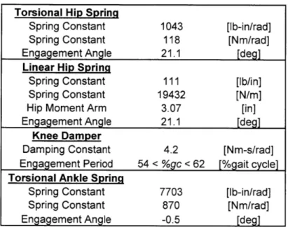
Passive elements were implemented in the exoskeleton to either store or dissipate energy with the objective of reducing the residual energy that the human would have to expend for locomotion. It was found that unidirectional springs should be implemented at the hip and ankle joints and a damper for the knee joint. Biomechanics data of the hip, knee, and ankle joints was analyzed to optimize the spring constants and damper values. The cost function was to minimize the residual power. Microsoft Excel's Solver was used as the optimizing method. The resulting spring constants and damper that were found are tabulated below in Table 2 along with the decrease in energy that they provided.

Torsional Hip Spring

Spring Constant 1043 [lb-in/rad]

Spring Constant 118 [Nm/rad]

Engagement Angle 21.1 [deg]

Energy Decrease 62 [%]

Linear Hip Spring

Spring Constant 111 [lb/in]

Spring Constant 19432 [N/m]

Hip Moment Arm 3 [in]

Engagement Angle 21.1 [deg]

Energy Decrease 62 [%]

Knee Damper

Damping Constant 4.2 [Nm-s/rad]

Engagement Period 54 < %gc < 62 [%gait cycle]

Energy Decrease 23 [%]

Torsional Ankle Spring

Spring Constant 7703 [lb-in/rad]

Spring Constant 870 [Nm/rad]

Engagement Angle -0.5 [deg]

Energy Decrease 50 [%]

Total Energy Decrease 46 [%]

Table 2 Summary of results from the passive element optimization

Several key assumptions were made in conducting this analysis. The data set used for the kinematic analysis was not exoskeleton data, but rather kinematic data from Natick Army Labs based on a participant walking normally and carrying a 47kg backpack [Harman (2000)]. It was decided that this data set could be used to analyze the exoskeleton to a first order approximation. It was also assumed that the gait kinematics remained unchanged despite the addition passive elements. Although, the passive elements may alter the kinematics since the exoskeleton is a dynamic system, the results of the analysis were still implemented as a first order approximation. Chapter 7 suggests acquiring biomechanic data directly from the exoskeleton with the passive springs implemented. This new data set would enable a more accurate kinematic analysis leading to more accurate passive element values.

2.2

Motivation

The power characteristics of the leg throughout the walking cycle suggest that it may be possible to implement passive elements at the hip, knee, and ankle joints to either store or dissipate energy throughout the walking cycle thus reducing the metabolic load on the human. Springs as energy storage elements can be implemented at joints that have a period of negative power followed by a period of positive power. The spring could store energy during the negative power period and release it during the positive power period. I hypothesize that with the introduction of passive elements to the exoskeleton joints, the human muscles would absorb less negative power and produce less positive power, thus providing metabolic advantages. The metabolic cost of absorbing power is 0.3 to 0.5 times that of producing power [De Looze et al. (1994)]. Dampers can be implemented for joints that mainly dissipate energy. These dissipative joints have a negative average joint power. The hip and ankle both have periods of negative power followed by a period of positive power and are candidates for implementing a spring to store and release energy throughout the gait cycle. The knee joint has a negative net average power throughout the gait cycle and is a candidate for implementing a damper.

MAN*

Ininal Contact Lowing Mid

TacclcalPr-wingTeg ative P Swerg

Figure 9 Negative and positive joint power during walking [Rab (1994)]

If a period of negative power precedes a period of positive power than it may be possible to capture the negative power in a spring and release it during the positive power period. This is such the case for the hip and ankle, where a spring may be implemented at these joints. The knee however, mostly dissipates energy

throughout the walking cycle and is best suited with a damper located at this joint.

Biomechanics data was analyzed to find the desired spring and damper values. The springs created a torque about the

joints reducing the torque required by the human. The

spring and damper values were optimized such that the residual power that human needed to exert was minimized.

Adding passive elements to the legs for walking has been studied previously by Antonie Bogert in 2003 and Daniel Paluska and Hugh Herr in 2004. Antonie Bogert developed a simulation of an exoskeleton that comprises of co-located pulleys at the hip, knee, and ankle

joints

and a long elastic cord that would wrap around the pulleys [van der Bogert (2003)]. Bogert optimized the pulley diameters to minimize the residual power that the human would need to exert. One case consisted of two 'exotendons', one for each leg, that span across three pulleys across all three leg joints. Another case used two six-joint 'exotendons' and 12 pulleys, where each 'exotendon' went across both legs. Dan Paluska and Hugh Herr looked at energetics of the ankle. Paluska and Herr analyzed

the ankle using Bogert's data and found that during specific periods of the gait cycle, an ankle could be modeled as a spring. For normal unloaded walking, they calculated a torsional ankle stiffness for a 70 kg person. Motivated by the human body's gastroc and soleus muscles, Paluska modeled a bi-articular clutched tendon that would involve the ankle and knee joints [Paluska (2004)]. His two-clutch, single tendon model was able to produce an energy savings similar to that of Bogert's 12 pulley model. These results from these individuals are summarized in the table below.

Leg Power

Reduction Stiffness

[%]

Bogert 3-joint exotendons, 6-pulleys, 2 tendons 47% Bogert 6-joint exotendons, 12-pulleys, 2 tendons 74% Paluska bi-articular clutched tendon , 4 tendons 75%

Paluska normal ankle stiffness result 300 [Nm/rad] 4.3 [Nm/rad-kg]

Table 3 Summary of results from Bogert and Paluska/Herr

The results from Bogert and Paluska reaffirm that it may be possible to implement springs in the exoskeleton to reduce the residual power required by the human for walking.

2.3 Biomechanics Data

2.3.1 Applying Backpack Data for Exoskeleton Analysis

After a careful literature search, loaded exoskeleton data was not available for analysis and design studies. Biomechanics data from Natick Army Labs [Harman et al. (2000)] comprising of ankle, knee, and hip torque as well as ankle and knee angle for walking carrying a 47 kg backpack was obtained. The Harman data is not exoskeleton data, but rather loaded walking data since the participant only walks with a loaded backpack. For the plots in this thesis, this data will be referred to as 'backpack'. An assumption is made that although walking with an exoskeleton may be significantly different than walking with a backpack, the kinematics and kinetics of the Natick backpack data can be applied to the exoskeleton for a first-order analysis. It was decided

to use the Natick data to analyze the biomechanics of the exoskeleton for optimizing the passive elements.

The Harman data set did not include hip angle data, but provided the maximum and minimum hip angles for walking with a 47 kg backpack. The hip angle from a normal walking data set [Bogert (2003)] was scaled to fit the maximum and minimum angle constraints specified by the Harman data set. The angle data for the knee and ankle for both the Bogert and Harman data sets are reasonably similar. Thus, scaling the Bogert hip data set is a reasonable first-order approximation to that of the actual hip angle for a participant carrying a 47 kg backpack.

The total mass of the exoskeleton is 15.5 kg and it carries a payload of 34kg (751b). The exoskeleton is capable of carrying a larger payload, but 75 lb was chosen as a representative load that a soldier or service personal may carry.

Approximately 6.5 kg of the exoskeleton mass is located around the hips, which would increase the effective backpack load to 40.5kg. An assumption is made that the biomechanics of a 40.5kg effective payload and a 9 kg net exoskeleton mass can be approximated by Harman's biomechanics data of carrying a 47 kg backpack. Table 4 summarizes the participants involved in the MIT and Natick studies.

Leg Walking

Participants Age Sex Payload Mass Length Speed

[n] [yr] [M/F] [kg] [kg] [im] [m/s] 34 load + 1 Participant 1 25 M 15.5exo 91 0.94 0.82 ±0.11 Natick / 16 Harman 30 ±9 16M OF 47 77 ±9 0.96 ±.04 1.33 ±0.18 several Bogert 0 70 0.9 1.2

Table 4 Summary of data used for analysis

The leg length and body mass for the Harman participants were reasonably close to that of the MIT test participant. The walking speed for the Harman data is 1.33 m/s and the MIT participant's speed was 0.82 m/s. Participant l's exoskeleton walking speed was self selected, while the Harman data's speed was matched to an average walking speed for humans carrying no load. The faster walking speed in the Harman data set would lead to higher torques and powers. Participant l's slower walking speed may result in a higher metabolic cost since the springs and dampers were optimized to the Harman data set.

Although the walking speed is different between the physical exoskeleton and the Harman data, the Harman data can be used to give a first-order approximation calculates the passive elements for the exoskeleton. To achieve more accurate results, it would be necessary to have biomechanics data measured directly from the exoskeleton for analysis. Acquiring this data is suggested in Chapter 7.

This thesis contains many plots and the convention for the 'x'-axis for most of them will be '% gait cycle,' which is time normalized. The following figure is a pictorial illustration of the gait cycle. The gait cycle begins with the heel strike.

_Ak_1_

"A

I

AAII

I

AA4kA

Right Left Left Right Right Left

Initial Pre- Initial Pre- Initial

Pre-Contact Swing Contact Swing Contact Swing

Time. pcivent of cycle

Double___ _ R. Single support u b - L. Single support D

Suppor suprtsppr

0"o41"Y 5(y% 9ry"6 100"%

r W Loo 50%tr I 0(s. Figure 10 Gait cycle for normal walking [Inman (1981)]

2.3.2 Summary of Data

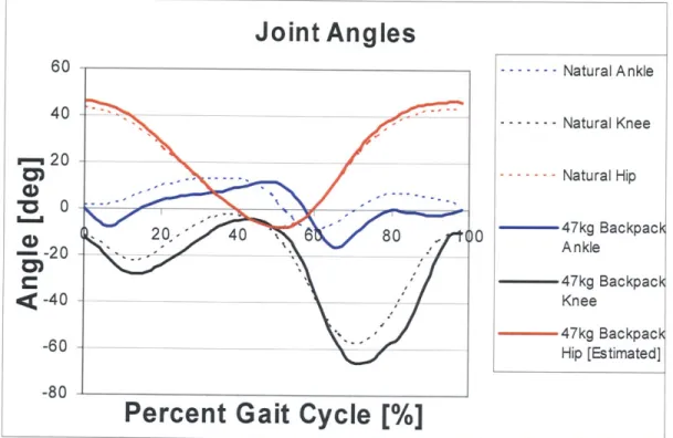
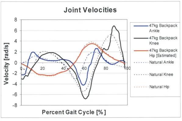
For the plots in this chapter, the data labeled 'Natural' (---) is the Bogert data set, and the data labeled '47 kg Backpack' (-) is the Harman data set from the Natick Army Labs. The Bogert data set is available online at [http://www.biomedical-engineering-online.com/content/2/1/17], and the Natick data is provided in the appendix of this thesis. Referring Figure 11 and Figure 12, it can be seen that the joint angle and velocity look similar to that of both the Bogert data and the Harman data. Based on qualitative experience looking at biomechanics data, the joint angle difference between the Bogert and Harman data sets are not significant. The joint velocities are slightly larger for the Harman data than that of the Bogert data, and this is because the Harman participants

walk at a speed that is 11% greater than that of the Bogert participants. For walking, the human legs act as an inverted pendulum and the body center of mass pivots over them [Farley et al. (1998)]. _{Intuitively, since the fundamental inverted pendulum walking} motion should not change with the addition of a load, it is reasonable to expect that the joint kinematics are similar.

Joint Angles

60 _{--- Natural Ankle} 40 -- _{--- Natural Knee} --- Natural Hip S0 20,- 40 80 . 00 47kgBackpac - -- -Ankle 47kg Backpack -40 _Knee 47kg Backpack -60 -_-_ - - - _{Hip [Estimated]} -80

Percent Gait Cycle

[%]

Figure 11 Joint angles, natural and 47 kg backpack

The joint angles for both normal and loaded walking are similar. The human kinematics are not substantially altered when walking with a loaded backpack.

Joint Velocities

8

_ - 47kg Backpack 6 - - - Ankle --- _47kg Backpack 4 Knee -- 47kg Backpack o Hip [Estimated] ..-..- N a t u r a l A n k le 20 40' 60 80 (C 0 --- ---...--- Natural Knee --- Natural Hip -6 -8

Percent Gait Cycle [%]

Figure 12 Joint velocities, natural and 47 kg backpack

The joint velocities for the Natick data are slightly larger than Bogert's since the participants for the Natick data walked 11% faster. The human kinematics are not substantially altered when walking with a loaded

backpack.

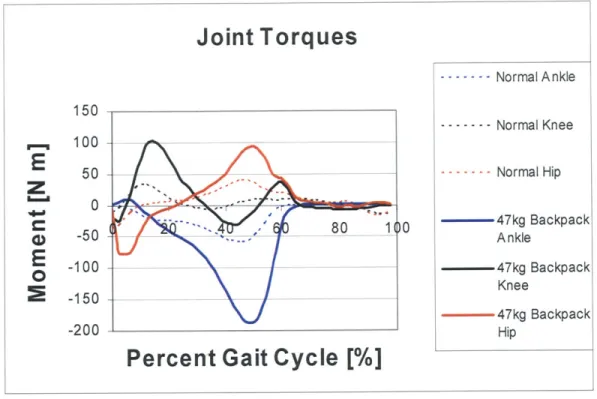
The backpack load did however increase the joint torque and power as compared to the normal unloaded case. This is reasonable since the added load increases the downward force significantly and translates into larger moments. If the walking speed is maintained, then the joint power will also increase since:

Joint Torques

-c---c 80 1

Percent Gait Cycle[%

--- Normal Ankle --- Normal Knee --- Normal Hip 47kg Backpack Ankle -- 47kg Backpack Knee 47kg Backpack Hip

Figure 13 Joint torques, natural and 47 kg backpack

The joint torques were larger for the backpack case compared to normal walking. This is expected since the larger forces are present due to the additional mass on the back.

Joint Power

400 300 200 100 0 0 -100 -200 -300 --- Normal Ankle -- NormalKnee --- _{Normal Hip} 47kg Backpack Ankle __ 47kg Backpack Knee ---- _47kg Backpack Hip

Percent Gait Cycle [%]

Figure 14 Joint power, natural and 47 kg backpack

The joint powers were larger for the backpack case compared to normal walking. This is also expected since larger forces are present due to additional mass on the back.

E

z

E

0 150 100 50 0 -50 -100 -150 -200 20 40- 60' 80 1

2.4 Analytical Methods

2.4.1 Optimizing the Hip and Ankle Springs

The backpack data from Harman was analyzed and optimized to determine how to implement a spring or damper to the exoskeleton to reduce the residual energy that the human would need to exert. Excel and Excel Solver were used to analyze and optimize the data. The optimization function is to minimize residual power that the human had to expend, which is the total joint power minus the passive element power. Optimizing residual power was chosen since the thesis goal is to reduce the human's metabolic cost of carrying a load. Joint torque, T, and joint angle, 0, were given by the Harman data for an average participant carrying a 47 kg backpack. Angular velocity was calculated by taking the derivative of angular position with respect to time. The walking period was not given but inferred from a chart that tabulated walking cadence, step length, and body height [Skinner (1994)]. The gait period was found to be 1.07 seconds.

* dO 0 =

dt _(2.2)

Mechanical power is calculated by:

P = T _(2.3)

A unilateral spring is chosen to be implemented for the exoskeleton hip and ankle. The unilateral spring would store and release energy during compression, but would be disengaged during extension. This one sided spring mechanism can be implemented simply by fixing the spring to only one of the members. Since the spring is unilateral it will only compress when the joint angle exceeds a specific threshold and transmit a torque. If the joint angle is less than the specified threshold angle, then the spring will not compress and energy will not be stored. The force in the spring is given by the following formula where '0' is the joint angle and 'k' is the spring constant.

k -(0 - Othreshold) if 0 > threshold

The spring force can be converted to a torque by multiplying by the moment arm between the location of the spring and the center of rotation of the joint, where 'r' is the moment arm length. If the moment arm is not included, as in the case for the ankle, then the spring constant 'k' is calculated as a torsional spring rather than a linear spring.

r -k -(0 - Othreshold) if 0 > Othreshold

Spring Torque = 0 if 0 < Othreshold (2.5)

The spring would reduce the torque and power required for locomotion. The residual torque and residual power that would be required by the human are given by the following formula where 'T' is the total torque required by the human.

R T -r -k -(0 - threshold) if 9 > Othreshold

Residual Torque = -rk(-TiO<hrsod (2.6)

T if 0 < threshold

Residual Mechanical Power T - r -k -(0 - Othreshold)]. if 0 > threshold

T*- if 0 < threshold

(2.7) It is assumed that adding a spring at the hip and ankle will not alter the leg kinematics. This is a major assumption since the exoskeleton is a dynamic system, and adding spring elements will most certainly affect the leg kinematics. Since modeling how the kinematics change cannot be easily analyzed, it is assumed for a first-order approximation that the kinematics will be approximately the same. For future work, it would be recommended to measure the joint kinematics with the springs implemented using a Vicon camera system, which is available at Spaulding Rehabilitation Center in Boston, MA.

Since the goal is to reduce the metabolic cost of load carrying and increase the endurance of the exoskeleton wearer, the cost function to be minimized is the average residual power that the human would have to expend. It has been shown that the metabolic cost related to negative work is 0.3-0.5 times that of positive work [De Looze (1994)]. As a conservative estimate, 0.5 will be used as a weighting factor on the negative power. Considering this, the residual power cost function to be minimized is:

F

Positive Re sidual + 0.5 -I

|Negative

Re sidual

1

MIN

L

ZTotal Positive + 0.5 -I|Total Negative|

And the percent savings is given by:

Positive Re sidual +0.5 - Negative Re sidual

(2.8)

-- (2.9)

following variables in Table 5 are adjusted in Excel Solver to minimize the power that the human had to exert.

a linear spring constant in [N/m] with a moment arm specified a torsional spring constant in [Nm/rad] with no moment arm

hreshold the spring engagement angle in [deg]

Table 5: Spring variables for residual energy minimization

Excel solver was used for the optimization and k and Otheshold were varied by Excel.

To implement a spring at a joint, it can be intuitively justified by looking at the power plots of the joints. These plots will be show later in this chapter. A spring can be implemented where there is a period of negative power followed by a period of positive power. This way, the spring can store energy during a period of negative power and release it during a period of positive power therefore reducing the power that the human leg would have to absorb or generate.

2.4.2 Optimization Algorithm for a Knee Damper

The exoskeleton knee joint mostly dissipates energy throughout the walking cycle. A damper in parallel with the human knee can dissipate the negative power and lessen the power that the human knee would have to absorb. Again, the optimization function is to minimize residual power that the human would have to expend. A rotary damper was chosen for the exoskeleton knee to provide a torque given by the following formula where 'B' is the dampening constant.

Damper Torque = B ~ 0

if

if

damper enabled damper disabled

It will be assumed that the damper can be enabled and disabled. The residual torque and residual power are therefore:

The residual ek ek .ot (2.10)

Residual Torque T - B -b if damper enabled (2.11)

T if damper disabled

Residual Mechanical Power = - B I damper enabled (2.12)

-T- if damper disabled

The cost function to minimize residual power for the damper case is equivalent to that of the spring case. The variables that can be adjusted to achieve the minimization are shown in Table 6. The gait cycle period was selected manually to match the large power spike in the swing-leg 'K4' region of Figure 16. Excel solver was used to vary the damping constant, 'B', to minimize the residual energy. Adding damping at the 'Ki' region was not considered for reasons that will be discussed in section 2.4.4.

" B the damping constant in [Nm-s/rad]

* %gsstar, %gsend % gait cycle when damper is engaged and disengaged

Table 6: Damper variables for residual energy minimization

Excel solver was used for the optimization and B varied by Excel. %gsstat, %gSend were selected manually and set during the region of largest negative power.

2.4.3 Hip Power

Referring to the 'hip power' plot in Figure 15, a spring can be placed to store the negative energy produced by the region 'H2' and released afterwards during the period 'H3'. It can also be seen that an engagement angle around 20 degrees should be expected.

Hip Power

0 0L 400 300 200 100 0 -100 -200 -300

-

i

-iI1

__Nh

20 .40 60'

Percent Gait Cycle [%] Possible Explanations:

pendulums over the

80 50 40 30 20 10 C 0 . 47kg Backpack Hip ----Hp Angle 1 -10 -20

Figure 15 Hip power [Harman et al. (2000)]

(HI) Positive Power - _{Stabilization during heel strike. (H2) Negative Power - Body} leg and stretches the quadriceps. (H3) Positive Power - Swinging the leg forward

400 300 200 10 0 0 -100 -20 -30 -40 0 0 -50

Knee Power

' - __ '',__- - - -10 K24 K4 0 -47kg Backpack Knee --- _Knee Angle II V20 60'1 KIK-200 - -- 6 -70 Percent Gait Cycle [%]

Figure 16 Knee power [Harman et al. (2000)]

Possible Explanations: (KI) Negative Power - _{Knee braking/bending after heel strike. (K2) Positive Power} - Knee straightening. (K3) Negligible Power - _{Body's inverted pendulum motion over the leg. (K4)} Negative Power - _{Knee bending during pre-swing and swing phase. (K5) Negative Power - Slowing of leg}

in terminal swing.

2.4.4 Knee Power

200 -0 - -60 -300

Referring to the 'knee power' plot in Figure 16, the only candidate period for a spring is in the 'K1-K2' region. This region is the period of walking that is shortly after heel strike when the knee quickly flexes and straightens during early stance. This quick flex and straightening motion is undesirable for the exoskeleton since it is preferred that the exoskeleton leg remain straight during this period. When the exoskeleton leg is completely straight, it acts as a column and all the downward vertical forces from the payload get transmitted through the exoskeleton leg. If the exoskeleton leg flexes after the heel strike impact, then the load bearing column effect is not supporting the load and the human leg has to bear the load. From wearing the exoskeleton, it is quite unpleasant when the exoskeleton is nicely carrying the payload and then for a split second the weight that the human has to support increases by 75 lbs. The 751b force spike may have adverse effects on the human gait and it is expected to not be metabolically efficient. Therefore, it is preferred that once the exoskeleton leg strikes the ground, it remains locked so that it can transfer the load to the ground while the body's center of mass pivots over the leg. If this walking cadence is executed correctly and the knee stays straight when the exoskeleton leg is on the ground then both the negative 'Ki' region and the positive 'K2' region are quite flat and almost non-existent. This leaves regions 'K3', 'K4', and 'K5' to be considered. It can be seen in Figure 16 that an integration of power over these three regions is negative and that a dissipative element is more fitting for these regions than a spring. If a dissipative element such as a damper is tuned correctly to absorb all the energy in the 'K4' region a metabolic advantage could be attained since that is power that the human leg does not have to absorb. Another idea is to still use a spring and store the negative power in the 'K4' region, and then through some mechanism transfer that energy to another joint that could benefit from it. This is exactly what motivated Dan Paluska and Hugh Herr with the bi-articular clutched tendons, which was discussed in section 2.2. Their approach was to transfer the energy from the 'K4' region of the knee to the ankle by means of a spring and two clutches [Paluska (2004)]. Implementing a functioning dual clutch tendon mechanism is not trivial, it was decided that for this thesis to simply use a damper and dissipate the energy. The variable-damping knee that was chosen was

developed by Hugh Herr and the MIT Leg Lab in the 1990's [Herr et al. (2003); Deffenbaugh et al. (2001)].

Integrating the knee power over the gait cycle shows that the overall knee power is largely negative. This observation is consistent for both the Harman and Bogert data sets.

47KG BACKPACK DATA (data from Harman)

Normalized Integrated Power

positive negative total %

energy energy energy positive

hip 0.16 0.13 0.29 0.56

knee 0.12 0.22 0.34 0.36

ankle 0.24 0.13 0.37 0.65

totals 0.53 0.47 1.00 0.53

NORMAL DATA (data from Bogert)

Normalized Integrated Power

positive negative total %

energy energy energy positive

hip 0.16 0.19 0.35 0.45

knee 0.07 0.25 0.32 0.22

ankle 0.26 0.07 0.34 0.78

totals 0.49 0.51 1.00 0.49

Table 7 Summary of positive/negative energy of joints

It can be seen that the knee mostly dominated by negative power. This motivates that a damper be implemented for the exoskeleton knee.

2.4.5 Ankle Power

The ankle has the largest peak power when compared to the other joints, so there is a definite advantage to minimizing residual power at this joint. Similar to the hip, it would be ideal if a spring element could capture the negative power of the 'Al' region and release it during the 'A2' peak. It is not intuitive as to what angle the ankle spring should engage at.

Ankle Power

400 ₁₅ 300 - - - 10 200 --- _-0- 547kg ---5 _Backpac M k A nkle 100 - - _{---- Ankle} A) Angle o 0 -5< 00 a. '' PA2 -100 - - - -10 -200 _-15 0 20 40 60 80 100 -300 -20

Percent Gait Cycle [%]

Figure 17 Ankle power [Harman et al. (2000)]

Possible Explanations: (Al) Negative Power - _{Extending ankle during heel strike. (A2) Positive Power} -Propulsive plantar flexion to thrust body forward and pre-swing the leg

2.5

Analytical Results

2.5.1 Summary of Results

The results from the aforementioned outlined analysis are summarized below. The hip results is given by both a torsional spring constant as well as a linear spring constant with a given moment arm. The hip engagement angle, when the spring starts to be compressed, is defined in front of the body (flexion). The knee result is given by a dampening constant and by a period of gait cycle when the damper should be activated. The ankle result is given by a torsional spring constant with an engagement angle of -0.5 degrees, which for practical purposes is 0.0 degrees, or when the ankle is at a right angle.