HAL Id: tel-01848542
https://tel.archives-ouvertes.fr/tel-01848542v3
Submitted on 14 Aug 2018HAL is a multi-disciplinary open access archive for the deposit and dissemination of sci-entific research documents, whether they are pub-lished or not. The documents may come from teaching and research institutions in France or
L’archive ouverte pluridisciplinaire HAL, est destinée au dépôt et à la diffusion de documents scientifiques de niveau recherche, publiés ou non, émanant des établissements d’enseignement et de recherche français ou étrangers, des laboratoires
Control-State Constraints and Delays
Riccardo Bonalli
To cite this version:
Riccardo Bonalli. Optimal Control of Aerospace Systems with Control-State Constraints and Delays. Optimization and Control [math.OC]. Sorbonne Université, UPMC University of Paris 6, Laboratoire Jacques-Louis Lions; ONERA – The French Aerospace Lab, Département TIS, Unité NGPA; Inria Paris, Equipe CAGE, 2018. English. �tel-01848542v3�
Paris 6 - Ecole Doctorale 386 UPMC - Laboratoire Jacques-Louis Lions
Thèse de Doctorat de Sorbonne Université
Présentée et soutenue publiquement le 13 juillet 2018
pour l’obtention du grade de
Docteur de Sorbonne Université
Spécialité Mathématiques Appliquées
par
Riccardo Bonalli
Optimal Control of Aerospace Systems with
Control-State Constraints and Delays
après avis des rapporteurs
M.
Jean-Baptiste Pomet
M.
Heinz Schättler
devant le jury composé de
M.
Jean-Baptiste Caillau
M.
Jean-Michel Coron
M.
Bruno Hérissé
M.
Romain Pepy
M.
Nicolas Petit
M.
Jean-Baptiste Pomet
M.
Emmanuel Trélat
Mme. Hasnaa Zidani
Examinateur
Examinateur
Encadrant
Membre invité
Examinateur
Rapporteur
Directeur de thèse
Examinateur
.
Talent is cheap; dedication is expensive. It will cost you your life.
Acknowledgements
These last three years have been filled up with many beautiful moments, involving love, work, passion and really important people. Let me devote some words to thank them all, by adopting the appropriate language.
Je souhaite tout d’abord remercier mon directeur de thèse Emmanuel Trélat et mon encadrant Bruno Hérissé. Ce travail n’aurait certainement pas pu être achevé sans leurs immenses supports.
La passion et la dévotion pour la recherche qui m’ont été transmises par Emmanuel sont pour moi une grande inspiration. Je tiens à le remercier encore pour son aide et sa grande disponibilité qui ont été au-delà de la direction de ce travail de thèse. L’aide et le soutien de Bruno ont été décisifs pour l’achèvement de ce travail. Il a su se montrer autant ami qu’encadrant et j’ai passé avec lui des moments très en-richissants aussi bien à l’ONERA qu’à l’extérieur.
Secondly, I would like to thank Mr. Jean-Baptiste Pomet et Mr. Heinz Schättler for their rich and precious reviews, allowing me to consistently improve this manuscript. Je tiens aussi à remercier chaleureusement tous les membres du jury pour avoir con-sacré leur précieux temps à l’écoute de ma soutenance de thèse.
Un remerciement très profond va à Cécile. Sa compréhension de ma passion et ses encouragements fondamentaux ont apporté le soutien décisif pour l’accomplissement de mes recherches. Aussi, elle m’a apporté les valeurs humaines qui composent sa belle personne, contribuant à mon évolution.
Ringrazio tutta la mia famiglia (italiana e "française"), e in particolare mia madre Cinzia, mio padre Marco e i miei fratelli Ursula e Leonardo. Il mio percorso, sia pro-fessionale che personale, è stato possibile grazie all’educazione dei miei genitori e alla fiducia che hanno sempre avuto in me.
Enfin, je veux remercier les doctorants de l’ONERA DTIS et tous mes amis pour les moments mémorables passés ensemble ces derniers trois ans ; en particulier, je re-mercie Aurore, Benjamin, Benoit, Camille, Carlos, David, Elinirina, Emilien, Evrard, Ioannis, Léon, Marlène, Parissay, Sergio, Simone, Sofyan et Vincent.
List of Publications
Journal Papers
• R. Bonalli, B. Hérissé and E. Trélat. Continuity of Pontryagin Extremals with
Respect to Delays in Nonlinear Optimal Control. Preprint, submitted to SIAM
Journal on Control and Optimization. https://arxiv.org/abs/1805.11990.
• R. Bonalli, B.Hérissé and E. Trélat. Optimal Control of Endo-Atmospheric Launch
Vehicle Systems: Geometric and Computational Issues. Preprint, submitted to
IEEE Transactions on Automatic Control. https://arxiv.org/abs/1710.11501.
Conference Papers
• R. Bonalli, B.Hérissé, H. Maurer and E. Trélat. The Dubins Car Problem with
Delay and Applications to Aeronautics Motion Planning Problems. 18th French
- German - Italian Conference on Optimization, 2017, Paderborn (Germany). • R. Bonalli, B.Hérissé and E. Trélat. Analytical Initialization of a
Continuation-Based Indirect Method for Optimal Control of Endo-Atmospheric Launch Vehi-cle Systems. IFAC World Congress, 2017, Toulouse (France).
• R. Bonalli, B.Hérissé and E. Trélat. Solving Optimal Control Problems for
De-layed Control-Affine Systems with Quadratic Cost by Numerical Continuation.
Contents
Introduction Générale 1
General Introduction 9
I Optimal Control Framework and Dynamical Model
17
1 Elements of Optimal Control 19
1.1 Some Tools from Differential Geometry . . . 19
1.1.1 Notations and Properties of Vector Fields . . . 19
1.1.2 Standard Results on Hamiltonian Fields . . . 21
1.2 Classical Optimal Control Problems . . . 23
1.3 Optimality Conditions and Numerical Methods . . . 25
1.3.1 The Maximum Principle . . . 25
1.3.2 Sufficient Optimality Conditions . . . 27
1.3.3 Classical Numerical Methods in Optimal Control . . . 29
1.3.4 Numerical Homotopy Methods . . . 31
1.4 Problems with Control and State Constraints . . . 34
1.4.1 General Control and State Constraints . . . 35
1.4.2 Mixed Control-State Constraints . . . 37
1.4.3 Numerical Difficulties Due to Control and State Constraints . . 40
1.5 Problems with Control and State Delays . . . 40
1.5.1 Maximum Principle for Problems with Delays . . . 40
1.5.2 Numerical Difficulties Due to Control and State Delays . . . 43
2 Rendezvous Problems 45 2.1 Physical Problem and Dynamical Model . . . 45
2.1.1 Fundamental Coordinate Systems . . . 45
2.1.2 Environmental and Dynamical Modeling . . . 48
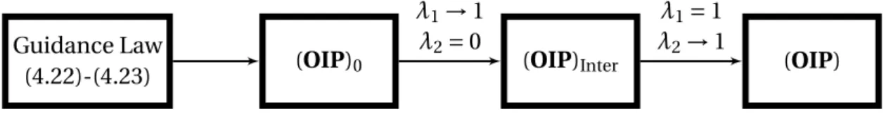
2.2.3 Optimal Interception Problem with Delays (OIP)τ . . . 57
II Structure of Extremals and Numerical Strategies of Guidance 59
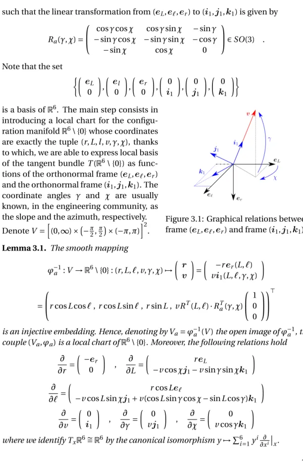
3 Structure of Extremals for Optimal Guidance Problems 61 3.1 Local Change of Problems Under Abstract Framework . . . 623.1.1 Reduction to Local Problems with Pure Control Constraints . . . 63
3.1.2 Sufficient Conditions Under Reduction to Local Problems . . . . 66
3.2 Local Transformations for (GOGP) . . . . 69
3.2.1 Coordinates Under the Trajectory Reference Frame . . . 70
3.2.2 Additional Local Euler Coordinates . . . 74
3.2.3 Global and Local Adjoint Formulations for (GOGP) . . . . 77
3.3 Regular and Nonregular Pontryagin Extremals . . . 80
3.3.1 Regular Pontryagin Extremals . . . 81
3.3.2 Nonregular Pontryagin Extremals . . . 84
3.4 Conclusions . . . 91
4 Numerical Guidance Strategy 93 4.1 General Numerical Homotopy Procedure for (GOGP) . . . . 94
4.1.1 General Optimal Guidance Problem of Order Zero (GOGP)0. . . 94
4.1.2 Parametrized Family of Optimal Control Problems (GOGP)λ . . 96
4.2 Optimal Interception Problem of Order Zero (OIP)0. . . 98
4.2.1 Approximated Local Controllability of (OIP)s0 . . . 101
4.2.2 From a LOS Analysis to a Suboptimal Guidance Law for (OIP)s0 . 103 4.3 Numerical Simulations for (OIP) . . . 105
4.3.1 Mathematical Design of the Mission . . . 105
4.3.2 Homotopy Scheme and Numerical Results . . . 107
4.4 Conclusions . . . 113
5 Numerical Robustness and Interception Software (ONERA) 115 5.1 Increasing the Robustness: Initialization Grids . . . 116
5.1.1 Fast Initialization Grids Design . . . 117
5.1.2 Numerical Time-Robustness Monte Carlo Experiments . . . 119
5.2 Software Design: a Template C++ Library (ONERA) . . . 123
5.2.1 Library Structure (Simplified UML Class Diagram) . . . 123
5.2.2 Details on Classes and User Script Examples . . . 123
III Continuity of Pontryagin Extremals with Respect to Delays 129
6 Solving Optimal Control Problems with Delays 1316.1 Continuity Properties with Respect to Delays . . . 132
6.2 Homotopy Algorithm and Numerical Simulations . . . 137
6.2.1 Solving (OCP)τby Shooting Methods and Homotopy on Delays 139 6.2.2 First Numerical Tests . . . 140
6.3 Numerical Strategy to Solve (OIP)τ . . . 144
6.3.1 Local Initialization Procedure for (OIP)τ . . . 146
6.3.2 Numerical Simulations for (OIP)τ . . . 148
6.4 Conclusions . . . 153
7 Continuity Properties of Pontryagin Extremals 155 7.1 Proof of the PMP Using Needle-Like Variations . . . 156
7.1.1 Preliminary Notations . . . 156
7.1.2 Needle-Like Variations and Pontryagin Cones . . . 157
7.1.3 Proof of The Maximum Principle . . . 160
7.2 Conic Implicit Function Theorem with Parameters . . . 161
7.3 Proof of Theorem 6.1 . . . 163
7.3.1 Controllability for (OCP)τ . . . 164
7.3.2 Existence of Optimal Controls for (OCP)τ . . . 165
7.3.3 Convergence of Optimal Controls and Trajectories for (OCP)τ . 168 7.3.4 Convergence of Optimal Adjoint Vectors for (OCP)τ . . . 172
7.4 Conclusions . . . 177
Conclusion 178 Bibliography 183 A Geometric Maximum Principle with State Constraints 195 A.1 Version of Theorem 1.3 Valid in Euclidean Spaces . . . 195
A.2 Some Useful Geometric Results . . . 198
A.3 Proof of Theorem 1.3 on Manifolds . . . 199
B Controllability Results 203 B.1 Local Controllability of (OIP)s0 . . . 203
B.2 Analysis of the Line Of Sight . . . 204
List of Figures, Tables and Algorithms 207
Résumé 208
Introduction Générale
Contexte Principal
Le guidage optimal des véhicules lanceurs a, au cours des dernières décennies, sus-cité de plus en plus l’attention, à tel point, qu’il est devenu un prérequis pour diverses applications aérospatiales, comme, le transfert orbital (voir, e.g. [1, 2]), la rentrée at-mosphérique (voir, e.g. [3, 4]) et le guidage de missiles (voir, e.g. [5, 6, 7, 8]).
Le problème a comme objectif de trouver une loi de contrôle permettant à un véhicule aérospatial de rejoindre une zone cible en considérant des contraintes spécifiques et des critères de performance. Les contraintes impliquent que seulement certaines manœuvres et trajectoires sont autorisées, et les critères de performance sont requis pour réduire les efforts et maximiser les chances de succès. Il est évident que ces contraintes et critères de performance dépendent du véhicule et de la mission. Par exemple, pour le transfert orbital, une des missions typiques consiste à déplacer un satellite sur une orbite déterminée, avec le minimum d’effort. Dans ce cas, les lois gravitationelles fixent des mouvements dynamiques précis. De plus, en raison du coût élevé des manœuvres en espace ouvert, on cherche à déplacer le satellite avec une consommation minimale de carburant. D’un autre côté, la mission d’interception consiste à mener un missile vers une cible (potentiellement rapide), en cherchant à la neutraliser. Dans cette situation, les contraintes sont données par l’équation de dynamique du vol et par la faisabilité de certaines manœuvres. Typiquement, on maximise la vitesse du véhicule pour augmenter les chances de détruire la menace. Le problème de guidage optimal peut être interprété, étudié et résolu à travers le for-malisme mathématique du contrôle optimal. Dans sa généralité, le problème con-siste à trouver un contrôle, comme fonction mesurable, pour un système dynamique évoluant sur une variété, tel qu’un coût lisse donné soit minimisé. Des contraintes, limitant aussi bien les contrôles que leurs trajectoires, sont souvent prises en compte. Les premiers apports à la théorie du contrôle optimal datent du 18ème siècle avec les travaux d’Euler et Lagrange, qui ont mené au calcul des variations. Cependant,
il a fallu attendre la fin des années 50 pour que les contributions de l’école russe de mathématiques fournissent les fondements théoriques pour le contrôle optimal de systèmes très généraux. Le travail novateur de Lev Pontryagin et de ses étudiants a apporté des conditions nécessaires d’optimalité puissantes, connues sous le nom du Principe de Maximum de Pontryagin (ou Principe de Maximum, ou encore PMP, voir, e.g. [9]), posant les bases de conditions plus exhaustives (voir, e.g. [10, 11, 12, 13, 14]). Dans le même temps, l’avancée de l’informatique et des méthodes numériques a permis de résoudre concrètement presque tout problème de contrôle optimal soumis par les applications et l’industrie, à l’exception d’erreurs numériques. Aujourd’hui, un large éventail d’algorithmes existe pour déterminer la solution de problèmes de contrôle optimal. Nous pouvons les classer en deux domaines principaux: méthodes directes et indirectes (voir, e.g. [15, 16, 17] pour plus de détails sur ces procédures). Les méthodes directes consistent à discrétiser les variables du problème de guidage optimal (l’état, le contrôle, etc.) pour le réduire à un problème d’optimisation non-linéaire sous contraintes. Un haut degré de robustesse est garanti et, de manière générale, aucune connaissance du système dynamique n’est nécessaire, entraînant une utilisation simple de ces méthodes en pratique. Cependant, leur efficience dépend fortement des capacités de calcul, impliquant une utilisation hors ligne le plus sou-vent. Par ailleurs, les méthodes indirectes consistent à appliquer les conditions don-nées par le Principe de Maximum en transformant le problème de guidage optimal en un problème aux valeurs limites. Les avantages de ces méthodes, dont la version basique est connue comme étant la méthode de tir, sont leur précision numérique extrêmement élevée et leur convergence rapide, si elle est atteinte. En revanche, l’initialisation de méthodes indirectes reste une tâche ardue.
Parmi les études menées par l’ONERA (Office National d’Etudes et de Recherches Aérospatiales), le guidage optimal de véhicules autonomes a acquis une position im-portante, à travers des applications civiles et militaires (lanceurs Ariane, systèmes de missiles, véhicules aériens sans pilote, etc.).
La plupart des travaux considèrent des calculs hors ligne à l’aide de méthodes di-rectes pour assurer une convergence robuste vers la solution optimale. Cependant, lorsqu’on traite de problèmes dynamiques, comme, par exemple, l’interception de cibles manœuvrantes, des trajectoires évaluées au préalable peuvent perdre rapide-ment leur optimalité, ou pire, mener à l’échec de la mission. Face à cela, une rééval-uation rapide des strategies optimales est nécessaire pour la réussite de la mission. Pour ces raisons, aujourd’hui, l’ONERA porte une attention particulière au développe-ment d’algorithmes pour le guidage optimal embarqué. Les nouvelles méthodes doivent être capables d’opérer efficacement avec des capacités computationnelles restreintes, permettant une mise à jour des calculs à une fréquence compatible de celle du guidage (souvent dans une gamme de 1-10 Hz).
Introduction Générale
Objectifs et Contributions de ce Travail
Ce travail est né d’une collaboration entre l’ONERA et le Laboratoire Jacques-Louis Lions (Sorbonne Université). L’objectif est de concevoir un algorithme autonome pour la prédiction de strategies de contrôle optimal concernant des missions à des-tination de véhicules lanceurs endo-atmosphériques. L’algorithme doit se baser sur des méthodes indirectes, et être capable de s’adapter à tout changement imprévu de scénario, en temps réel. L’intérêt principal se trouve dans les missions d’interception. Le choix des méthodes indirectes dérive du fait qu’elles sont bien adaptées pour ap-porter une forte précision numérique et une rapidité de calculs, idéales pour des opérations embarquées. Un autre point important consiste à assurer la mise en place de strategies pour chaque scenario potentiellement réalisable. De plus, la robustesse des algorithmes concernés doit être assurée au moins statistiquement.
Pour atteindre cet objectif, nous avons identifié les étapes et contributions suivantes: 1. Appliquer le Principe du Maximum pour des stratégies globales.
Une étude précise du guidage optimal de véhicules lanceurs nécessite de pren-dre en compte de lourds critères de performance, ainsi que des missions diffi-ciles. Etant donné que dans cette situation le véhicule est sujet à de nombreux efforts mécaniques, differentes contraintes de stabilité doivent être imposées, faisant ainsi apparaître des contraintes mixtes, c’est-à-dire, combinant à la fois des variables de contrôle et d’état. Ce type de problème de contrôle optimal est difficile à traiter par le Principe de Maximum (voir, e.g. [12, 18]). En ef-fet, d’autres multiplicateurs de Lagrange apparaissent, pour lesquels, obtenir des informations rigoureuses et utiles peut être compliqué, cela a été l’objet de multiples études (voir, e.g. [19, 20, 21]). Cette complication empêche de pou-voir considérer des méthodes indirectes basiques, compromettant une conver-gence rapide vers les solutions optimales.
L’approche largement diffusée en aéronautique, permettant d’éviter de traiter des contraintes mixtes, consiste à reformuler le problème original de guidage en utilisant des coordonnées locales d’Euler, sous lesquelles, la contrainte de stabilité devient une contrainte pure de contrôle (voir, e.g. [22]). Cette trans-formation permet de considérer le Principe de Maximum classique, donc, les méthodes usuelles de tir. En revanche, les coordonnées d’Euler ne sont pas globales et ont des singularités, empêchant la resolution de toutes configura-tions réalisables, et réduisant le nombre de missions achevables.
optimal dans un point de vue intrinsèque, en utilisant le contrôle géometrique (il n’apparaît pas que ce cadre ait été systématiquement étudié dans le contexte du guidage optimal). En particulier, nous construisons des coordonnées lo-cales supplementaires, couvrant les singularités de ces dernières, sous lesquelles la contrainte mixte peut être toujours réinterprétée comme une contrainte pure de contrôle. De plus, ces deux ensembles de coordonnées locales constituent un atlas de la variété en question, que nous utilisons aussi pour découvrir, en exploitant des outils de contrôle géométrique, le comportement complet des extrémaux de Pontryagin, aussi dans le cas d’arcs non réguliers.
L’introduction de ces coordonnées locales particulières engendre deux béné-fices principaux. D’un côté, il n’y a pas de limite aux scénarios faisables pou-vant être simulés. D’un autre côté, le problème de guidage optimal n’est pas conditioné par des multiplicateurs dépendants de contraintes mixtes (ou, au moins, localement), donc, les méthodes indirectes classiques peuvent être facile-ment mises en pratique. C’est au prix du changefacile-ment de coordonnées lo-cales, qui complexifie légerement l’implementation de la méthode de tir, mais, n’influence pas de manière importante la vitesse et la précision computationelles. 2. Concevoir un chemin numérique efficace basé sur des méthodes indirectes.
La procédure détaillée précedemment nous permet d’appliquer les méthodes indirectes pour résoudre des problèmes de guidage optimal. Cependant, comme il a déjà été relevé, même si les méthodes indirectes ont une très bonne préci-sion numérique, leur défaut principal reste leur initialisation. Cette probléma-tique est bien connue dans la communauté aérospatiale et beaucoup d’efforts ont été faits pour permettre des procédures d’initialisation efficaces (on trouve un résumé approfondi de ces techniques dans la revue [23]). Le but étant de garder l’algorithme de résolution indépendant des méthodes directes, nous souhaitons éviter l’utilisation de ces dernières.
Nous proposons une procédure d’initialisation efficace pour méthodes indi-rectes par l’emploi des méthodes d’homotopie (voir, e.g. [24]). Récemment, ces schémas numériques ont acquis une bonne réputation dans les applica-tions aérospatiales, principalement grâce à leur haute fiabilité et polyvalence (voir, e.g. [25, 26, 27]). L’idée de base des méthodes d’homotopie est de ré-soudre un problème difficile, étape par étape, en commençant par un prob-lème simple (usuellement appelé probprob-lème d’ordre zéro), par déformation de paramètre. Associé au tir provenant du Principe de Maximum, une méthode d’homotopie consiste à déformer le problème aux valeurs limites en un plus simple (qui peut être facilement résolu), puis, résoudre une série de tirs, étape par étape, en remontant au système original. Dans le cas où le paramètre d’homotopie est un nombre réel et le chemin est constitué d’une
combinai-Introduction Générale
son convexe du problème d’ordre zéro et original, la méthode d’homotopie est plutôt appelée méthode de continuation.
Les méthodes d’homotopie numériques sont composées par deux principales étapes: le choix d’un problème d’ordre zéro (qui devrait être le plus facilement résoluble possible) et d’une procédure de déformation de paramètre. Nous résolvons le problème de guidage optimal en adoptant le schéma suivant:
2.a) Concevoir et résoudre le problème d’ordre zéro par une loi explicite. Des tests expérimentaux démontrent que le problème de guidage opti-mal simplifié, obtenu en retirant les contributions de la poussée et de la gravité du modèle dynamique initial, conserve des régularités suffisantes, afin, qu’une fois que ce problème d’ordre zéro soit déterminé, une défor-mation de paramètre appropriée permet une convergence rapide de la procédure d’homotopie. En outre, l’initialisation des méthodes de tir sur ce problème de guidage optimal simplifié peut être faite analytiquement et instantanément. En effet, en manipulant le Principe du Maximum ap-pliqué à ce problème, nous fournissons une nouvelle loi de guidage ca-pable d’initialiser efficacement des méthodes indirectes sur le problème d’ordre zéro précédent, pour un large éventail de scénarios.
2.b) Concevoir un schéma approprié de déformation de paramètre.
Le problème original de guidage optimal est résolu en déformant le prob-lème d’ordre zéro précédent, par un ajout itératif de la poussée et de la gravité précédemment retirées. Nous choisissons un scénario modifié ca-pable d’initialiser analytiquement le problème simplifié (voir 2.a)) en le gardant fixe pendant cette étape d’homotopie. Par la suite, une dernière étape d’homotopie modifie le scénario temporaire pour obtenir la solu-tion de l’intégralité du problème considérant le scenario original.
Lorsque le scénario implique que la trajectoire optimale rencontre des singu-larités d’Euler, dans le schéma numérique précédent, les calculs sont tempo-rairement arrêtés et un changement de coordonnées est opéré (voir 1.). A partir de cela, l’intégration numérique reprend en évitant des échecs de convergence. Ce changement de coordonnées affecte peu le temps computationnel total, en maintenant le taux classique de convergence des méthodes indirectes.
3. Renforcer et accélérer la convergence pour le problème de guidage.
Même si les procédures numériques développées en 2. fournissent un schéma efficace pour résoudre le problème de guidage optimal de véhicules lanceurs, une problématique reste à régler: la haute sensibilité aux conditions initiales.
En effet, toute la procédure d’homotopie décrite en 2., qui commence du prob-lème simplifié et finit avec l’étape de déformation du scénario, peut contenir plusieurs itérations homotopiques (dépendant de la difficulté de la mission). Cela implique que différentes missions peuvent prendre plus ou moins de temps computationnel pour converger vers la solution optimale. En d’autres termes, le temps computationnel moyen de ce schéma d’homotopie peut être trop long pour une implémentation en temps réel.
Comme solution, nous proposons de traiter le probème lié à la haute sensibil-ité, et donc améliorer la robustesse du schéma d’homotopie, en utilisant une grille raffinée de guesses initiaux, évaluée hors ligne, qui contient les solutions du problème complet original (poussée et gravité incluses) pour plusieurs scé-narios réalisables. Puis, la résolution de toutes missions arbitraires procède de la manière suivante. Premièrement, la grille est chargée dans la RAM (hors ligne). En suite, le scénario le plus proche (par rapport à une certaine métrique) de celui fourni par l’utilisateur est sélectionné à partir de la grille d’initialisation. Finalement, une déformation spatiale est mise en place pour récupérer la so-lution du problème original. Plus la grille est fine, meilleure est la chance d’obtenir une solution optimale globale.
Nous développons cette amélioration dans le contexte de l’interception op-timale. Des tests statistiques montrent que seulement peu d’itérations homo-topiques sont nécessaires en général pour obtenir une solution, donc, de hauts taux de convergence sont assurés. De plus, comme la réévaluation de strate-gies d’interception est assez élevée, la robustesse des solutions par rapport aux variations extérieures du scénario initial, comme des cibles mouvantes, aug-mente considérablement.
4. Caractère bien posé des méthodes d’homotopie pour les problèmes de con-trôle optimal avec retards, lorsque l’homotopie est opérée sur les retards. Les problèmes de guidage optimal se focalisent sur le contrôle de la dynamique du centre de gravité des véhicules lanceurs, en évitant de traiter le contrôle des configurations du corps rigide. Plusieurs raisons sont invoquées pour consid-érer séparément le problème de guidage et les manœuvres réalisées par le pi-lote. Celle faisant l’unanimité atteste que, généralement, le système de guidage opère à une fréquence plus faible que celle du pilote. En revanche, certains re-tards apparaissent dans le suivi des consignes. Pour améliorer le modèle et les lois de contrôle, on peut étendre le problème de guidage optimal en approx-imant l’action du pilote dans les équations de mouvement, et en considérant des retards entre la translation et la rotation (voir, e.g. [6, 28]).
Ce contexte oblige à gérer des problèmes de contrôle optimal non linéaires avec retards et le défi consiste à résoudre efficacement ces problèmes par des
Introduction Générale
algorithmes de tir. Cette question est habituellement complexe et computa-tionnellement coûteuse. En effet, le Principe de Maximum pour problèmes de contrôle optimal avec retards (voir, e.g. [29, 30, 31, 32]) conduit à des prob-lèmes aux valeurs finales qui combinent des termes antérieurs et postérieurs du temps, en obligeant une intégration globale des équations différentielles annexes. Un guess local concernant l’extrémale optimale n’est plus utile, un guess global doit plutôt être fourni pour permettre la convergence de la procé-dure. Cela représente une autre difficulté par rapport aux méthodes de tir usuelles, et affecte clairement les performances computationnelles.
Comme les méthodes précédemment adoptées permettent de résoudre le prob-lème de guidage optimal sans retards, il semble légitime de se demander si on peut résoudre le problème de guidage optimal contenant des retards par des méthodes indirectes, en commençant une procédure d’homotopie dans laquelle le délai représente le paramètre de déformation, et le problème sans retards est considéré comme le problème d’ordre zéro. Cette approche est un moyen possible pour traiter le défaut des méthodes indirectes appliquées aux problèmes de contrôle optimal avec retards: d’une part, l’information globale donnée par le problème sans aucun retard pourrait être utilisée pour initialiser efficacémment une méthode de tir avec retards; d’autre part, nous pourrions résoudre le problème aux valeurs limites avec retards à l’aide de méthodes itératives locales pour équations différentielles. Nonobstant, différemment du contexte classique du contrôle optimal sans retards, pour lequel, sous des hy-pothèses appropriées, la convergence des méthodes d’homotopie est comprise et bien établie (voir, e.g. [23]), le caractère bien posé des méthodes indirectes combinées avec des procédures d’homotopie sur le retard n’a pas encore été bien traité dans la littérature. En particulier, des points de bifurcation ou des singularités peuvent apparaître, entraînant des échecs de convergence.
La solution que nous proposons réside sur une étude détaillée du caractère bien posé des procédures d’homotopie pour résoudre des problèmes généraux de contrôle optimal non-lineaires avec retards, par des méthodes indirectes. Notre principal resultat théorique est que, sous des hypothèses appropriées, les quantités fournies par le Principe de Maximum, incluant les vecteurs ad-joints et les trajectoires, sont continues par rapport aux retards. Ce résultat assure le caractère bien posé du schéma numérique proposé précédemment: tout chemin d’homotopie sur les retards converge vers les extrémaux de Pon-tryagin du problème de contrôle original avec retards, si on part du problème sans aucun délai. Une fois ces propriétés de continuité établies dans un con-texte général, nous exploitons ce résultat pour fournir efficacement une réso-lution numérique pour problèmes de guidage optimal avec retards.
complètement automatique, indépendant et auto-régulé, aujourd’hui propriété de l’ONERA, pour des applications réalistes dans le cadre de véhicules lanceurs, focal-isé, en particulier, sur des scénarios d’interception optimal. En une seule seconde, l’algorithme est capable de fournir des strategies optimales pour onze missions dif-férentes avec juste un processeur de quelque mégabyte de mémoire, permettant des calculs en temps réel, idéal pour des véhicules autonomes.
Organisation du Manuscrit
Ce travail s’organise en sept chapitres et une conclusion finale.
Les chapitres 1 et 2 ont comme objectif d’introduire au lecteur la théorie classique du contrôle optimal et les problèmes de guidage sur lesquels cette étude se concentre. Dans un même temps, ces chapitres fournissent les notations et résultats théoriques standards utilisés tout au long de ce manuscrit.
Dans le Chapitre 3, nous dérivons la structure des extrémaux de Pontryagin du prob-lème de guidage optimal. Un contexte abstrait introduisant les conditions de con-sistance des vecteurs adjoints sous transformations locales est d’abord présenté. Le résultat est alors appliqué pour une étude correcte des contrôles réguliers et non réguliers, à travers le Principe de Maximum, dans le contexte du guidage optimal. Les chapitres 4 et 5 concernent le développement et les améliorations annexes des stratégies numériques pour le guidage optimal de missiles intercepteurs, à travers les méthodes indirectes. Dans le Chapitre 4, la méthode indirecte classique est com-binée avec un schéma d’homotopie efficace, dont l’initialisation est apportée à l’aide d’une étude additionnelle de certaines formulations approchées du Principe de Max-imum. Le Chapitre 5 propose l’amélioration de la robustesse numérique via la con-struction de grilles d’initialisation.
La strategie numérique pour résoudre les problèmes de contrôle optimal avec re-tards, en combinant les méthodes indirectes et l’homotopie sur les rere-tards, est intro-duite et analysée dans les chapitres 6 et 7. Le Chapitre 6 fournit d’abord les propriétés de continuité, par rapport au retard, des extrémals de Pontryagin liées aux problèmes de contrôle optimal avec retards. Donc, sur la base de ces résultats, l’algorithme d’homotopie annexe est introduit et commenté à l’aide de simulations numériques concernant des problèmes de guidage optimal plus généraux. D’autre part, le Chapitre 7 est consacré aux détails de la preuve des propriétés de continuité précédentes. Enfin, le manuscrit s’achève par une section dédiée aux conclusions et perspectives.
General Introduction
Main Context
The optimal guidance of launch vehicles has attracted more and more attention in the past few decades, so that, nowadays, it has become literally a prerequisite in vari-ous aerospace applications, such as, orbit transfer (see, e.g. [1, 2]), atmospheric entry (see, e.g. [3, 4]) and missile guidance (see, e.g. [5, 6, 7, 8]).
This problem is devoted to finding a control law enabling an aerospace vehicle to join a final target area by considering prescribed constraints as well as performance criteria. Constraints mean that only certain maneuvers (i.e. controls) and trajectories are allowed while performance criteria are demanded to reduce expensive efforts or maximize chances of success. Of course, these constraints and performance criteria depend on the considered vehicle and, as well, on the mission to accomplish.
For instance, in orbit transfer applications, a typical mission consists in steering a satellite from a halo to another given orbit, with minimal effort. In this case, gravita-tional laws provide precise dynamical movements to which the vehicle is confined. Moreover, due to the high cost of even small maneuvers in open space, one usually tries to displace the satellite by minimal fuel consumption. On the other hand, inter-ception missions consist in leading a missile towards a (possibly fast) target (cruise missile, ballistic missile, etc.), with the aim of neutralizing it. In this situation, con-straints are given by the equations of flight dynamics and by the feasibility of certain maneuvers. Typically, one makes further efforts to maximize the velocity of the vehi-cle, in order to increase lethality and chances to destroy the threat.
Optimal guidance problems can be interpreted, studied and solved via the formal and well-posed mathematical representation given by optimal control. In its gener-ality, classical optimal control deals with the problem of finding a measurable control function for a given control dynamical system, evolving within a manifold, such that a certain smooth cost functional is minimized. Constraints, limiting either the con-trol functions or the dynamical trajectories, are usually taken into account.
The first answers to optimal control problems date back to the 18th century with the work done by Euler and Lagrange, which led to the calculus of variations. However, it is in the late 50s of the last century that the contributions of the Russian school of mathematics provided the theoretical fundamental results for the optimal control of very general control systems. The pioneering work of Lev Pontryagin and his stu-dents yielded powerful necessary optimality conditions, known as Pontryagin Max-imum Principle (or just MaxMax-imum Principle, or PMP, see, e.g. [9]), and put the basis for more exhaustive conditions (see, e.g. [10, 11, 12, 13, 14]).
Simultaneously, the advent of computers and numerical methods allowed to practi-cally solve almost every optimal control problem provided by applications and com-panies, up to numerical approximation errors. Nowadays, a large spectrum of nu-merical algorithms exist to provide solutions to optimal control problems, and we can roughly split them into two main classes: direct methods and indirect methods (see, e.g. [15, 16, 17] for detailed surveys on these numerical procedures).
Direct methods consist in discretizing each component of the optimal guidance prob-lem (the state, the control, etc.) to reduce it to a nonlinear constrained optimization problem. A high degree of robustness is provided while, in general, no deep knowl-edge of the dynamical system is required, making these methods rather easy to use in practice. However, their efficiency strongly depends on computational capabili-ties, which often obliges to use them offline uniquely. On the other hand, indirect methods consists in applying the conditions given by the Maximum Principle, wrap-ping the optimal guidance problem into a two-point boundary value problem, which leads to accurate and fast algorithms. The advantages of indirect methods, whose more basic version is known as shooting method, are their extremely good numerical accuracy and the fact that, if they converge, the convergence is very quick. Neverthe-less, initializing indirect methods still remains the hardest task.
Among research studies carried out at ONERA-The French Aerospace Lab, optimal guidance of launch vehicles has earned an important position, finding both civil and military applications (launch systems such as Ariane rockets, missile systems, un-manned aerial vehicles, etc.).
Most of the main frameworks consider offline computations via direct methods to ensure robust convergence to optimal solutions. However, when managing dynamic problems such as, for example, an interceptor missile dealing with maneuvering tar-gets, precomputed trajectories can lose quickly their optimality, or worse, lead to a failure of the mission. In this situations, fast recomputations of optimal trajectories are needed to definitely improve the chances to achieve the mission.
For these reasons, today, ONERA-The French Aerospace Lab devotes particular at-tention on the development of algorithms for an onboard real-time optimal guidance of launch vehicles. Onboard means that the new methods should be able to operate
General Introduction
efficiently with a reduced charge of processors, while real-time implies the ability to provide online updates of numerical computations at frequencies compatible with the operating frequency of the guidance system (usually in the range of 1-10 Hz).
Objective and Contributions of this Work
The present work arises from a collaboration between ONERA-The French Aerospace Lab and LJLL-Laboratoire Jacques-Louis Lions (at Sorbonne University). The main objective consists in conceiving an autonomous algorithm for the prediction of opti-mal control strategies for endo-atmospheric launch vehicle missions, based on indi-rect methods, and able to adapt itself to unpredicted changes of the original scenario, in real time. Particular interest is put on interception missions.
The choice of preferring indirect methods to compute optimal trajectories derives from the fact that they are well-suited to provide both good numerical accuracy and real-time compatibility, ideal for onboard processors. Another important require-ment is to ensure that the whole method provides strategies for every feasible sce-nario. Robustness of the concerned algorithms must be ensured at least statistically. To this aim, we identify the following main goals and related contributions:
1. Apply the Maximum Principle and recover global strategies.
An accurate study of the optimal guidance of endo-atmospheric launch ve-hicles compels to consider both usually demanding performance criteria and possible onerous missions to accomplish. Since, in this situation, the vehicle is subject to several strong mechanical strains, some stability constraints must be imposed, which turn out to be modeled as mixed control-state constraints, i.e. combined constraints limiting both controls and trajectories. This kind of optimal control problems is difficult to treat by the Maximum Principle (see, e.g. [12, 18]). Indeed, further Lagrange multipliers appear, for which, obtain-ing rigorous and useful information may be arduous and has been the object of many studies in the existing literature (see, e.g. [19, 20, 21]). This issue pre-vents from considering usual indirect methods, therefore, compromising fast convergences to optimal solutions.
A widespread approach in aeronautics to avoid to deal with these particular mixed control-state constraints consists in reformulating the original guidance problem using some local Euler coordinates, under which, the stability con-straints become pure control concon-straints (see, e.g. [22]). The transformation allows to consider the classical Maximum Principle, and then, usual shooting methods. However, Euler coordinates are not global and have singularities that
prevent from solving all reachable configurations, reducing the number of pos-sible achievable missions.
The solution that we propose consists in reformulating the optimal guidance problem within an intrinsic viewpoint, using geometric control (it does not seem that this general framework has been systematically investigated in the optimal guidance context so far). In particular, we build additional local co-ordinates which cover the singularities of the previous ones and under which the mixed control-state constraints can still be reinterpreted as pure control constraints. Moreover, these two sets of local coordinates form an atlas of the configuration manifold which we use also to recover, by using some geometric control techniques, the complete behavior of Pontryagin extremals, even in the case where nonregular arcs occur.
The introduction of these particular local coordinates provides, in turn, two main benefits. On one hand, there is no limit on the feasible mission scenarios that can be simulated, and, on the other hand, the optimal guidance problem is not conditioned by multipliers depending on mixed constraints (or, at least, lo-cally), therefore, classical standard indirect methods can be easily put in prac-tice. This is at the price of changing local coordinates, which slightly compli-cates the implementation of the shooting method, but, importantly, does not affect its computational speed and precision.
2. Design an efficient numerical scheme based on indirect methods.
The procedure detailed previously allows to apply indirect methods to solve endo-atmospheric optimal guidance problems. However, as already pointed out, even if indirect methods have extremely good numerical accuracy, their main drawback is their initialization. This issue is well-known in the aerospace community and many efforts were gathered to provide efficient initialization procedures (a thorough summary of these techniques can be found in the sur-vey [23]). Since the aim is to keep the whole resolution algorithm independent from direct methods, we desire to avoid the use of any kind of direct method. We propose an efficient initialization procedures for indirect methods by em-ploying homotopy methods (see, e.g. [24]). Recently, these numerical schemes have acquired good reputation for aerospace applications, mostly thanks to their high reliability and versatility (see, e.g. [25, 26, 27]). The basic idea of homotopy methods is to solve a difficult problem step by step starting from a simpler problem (usually called problem of order zero) by parameter deforma-tion. Combined with the shooting problem derived from the Maximum Princi-ple, a homotopy method consists in deforming this two-point boundary value problem into a simpler one (which can be easily integrated) and then solving a series of shooting problems step by step to come back to the original system.
General Introduction
In the case in which the homotopic parameter is a real number and when the path consists in a convex combination of the problem of order zero and of the original problem, the homotopy method is rather called continuation method. Numerical homotopy methods are composed by two main steps: the choice of a problem of order zero (which should be as simple to solve as possible) and a procedure for the parameter deformation. We solve numerically the endo-atmospheric optimal guidance problem by adopting the following scheme:
2.a) Design and solve the problem of order zero by an explicit guidance law. Experimental tests show that the simplified optimal guidance problem obtained by removing the contribution of the thrust and the gravity from the original flight dynamical model maintains sufficient regularities, so that, once this problem of order zero is solved, appropriate parameters deformations on it result in a fast converging homotopy procedure. Another important property of this simplified optimal guidance problem is that initializing shooting methods on it can be done analytically and in-stantaneously. Indeed, by manipulating the Maximum Principle applied to this problem, we provide a new approximated explicit guidance law able to efficiently initialize indirect methods on the previous problem of order zero, for a large range of initial and final conditions.
2.b) Devise an appropriate parameter deformation scheme.
The original optimal guidance problem is solved deforming the previous problem of order zero by adding iteratively the contribution of the thrust and the gravity previously removed. We choose a modified feasible sce-nario able to initialize the simplified problem analytically (see 2.a)) and keep it fixed during this homotopy step. Therefore, one further homotopy step deforms the first temporary scenario to obtain the optimal solution of the complete problem considering the original scenario.
When the scenario implies that the optimal trajectory encounters some Euler singularity, in the previous numerical scheme, the computations are temporar-ily stopped and a change of coordinates is operated (see 1.). From this, the numerical integration starts again avoiding converging failures. This change of coordinates slightly affects the total computational time, maintaining the usual fast convergence rate of indirect methods.
3. Robustify and speed up the convergence of the guidance problem.
Even if the numerical procedure developed in 2. provides an efficient scheme to solve the optimal guidance of launch vehicles, one main issue is not figured
out: the high sensitivity to initial conditions. Indeed, the whole homotopy pro-cedure described in 2., starting from the simplified problem and finishing with the scenario deformation step, may contain several homotopic iterations (de-pending on the difficulty of the mission), implying that different missions may take more or less computational time to converge to the optimal solution. In other words, the average computational time of the whole homotopy scheme may be too large for a real-time implementation.
As solution, we propose to manage the high sensitivity issue, thus increasing the robustness of the homotopy scheme, by calling a refined offline precom-puted grid of initial guesses of Pontryagin extremals, that contains the solu-tions of the complete original control problem (thrust and gravity included) for many feasible scenarios. Therefore, the resolution of any given arbitrary mission proceeds as follows. First, the grid is charged into the RAM (offline), then, the scenario the closest (with respect to some metric) to the one provided by the user is selected from the initialization grid, and finally, a spatial defor-mation is computed to recover the solution of the original problem. The finer the grid is, the better chance one has to obtain the global optimal solution. We develop this improvement in the context of optimal interception missions. Statistical numerical tests show that only few homotopic iterations are needed in general to obtain a solution, thus high rates of convergence are ensured. Furthermore, since the recomputing of interception strategies is fast enough, the robustness of solutions with respect to exterior variations of the initial sce-nario, such as fast moving targets, increases considerably.
4. Discuss and prove the well-posedness of homotopy methods for optimal con-trol problems with delays, when the homotopy is operated on delays.
Optimal guidance problems focus on the control of the dynamics of the center of gravity of launch vehicles, avoiding to manage the control of rigid body con-figurations. Several reasons are invoked to consider separately the guidance problem and the physical maneuvers realized by the pilot, and the most unan-imous one states that, usually, the guidance system operates at lower frequen-cies than the pilot. However, some delays on the follow-up of orders occur. In order to refine the model and related control laws, one can extend the opti-mal guidance problem by approximating the contribution of the pilot (i.e. of the rigid body dynamics) into the equations of motion, and considering delays between the translating dynamics and the rotating dynamics (see, e.g. [6, 28]). This framework obliges to deal with nonlinear optimal control problems with delays and the challenge consists in solving efficiently such problems by shoot-ing algorithms. This question is usually complex and computationally demand-ing. Indeed, the Maximum Principle for optimal control problems with delays
General Introduction
(see, e.g. [29, 30, 31, 32]) provides nonlinear two-point boundary value prob-lems which combine backward and forward terms of time, forcing a global in-tegration of related differential equations. Therefore, a local guess concerning the optimal extremal is no more useful, but rather, good global guesses must be provided to make the procedure converge. This represents an additional diffi-culty with respect to the usual shooting method, which clearly affects compu-tational performances.
Since the methods previously adopted allow to solve the optimal guidance prob-lems without delays, it seems legitimate to wonder if one may solve the opti-mal guidance problem containing delays by indirect methods starting a homo-topy procedure where the delay represents the deformation parameter and the problem without delays is taken as the problem of order zero. This approach is a way to address the flaw of indirect methods applied to optimal control prob-lems with delays: on one hand, the global information of the problem without any delay could be used to initialize efficiently a shooting method with delays and, on the other hand, we could solve the two-point boundary value problem with delays via usual local iterative methods for differential equations. Never-theless, unlike the classical non-delayed optimal control framework, in which, under appropriate assumptions, the convergence of homotopy methods is un-derstood and well-established (see, e.g. [23]), the well-posedness of indirect methods combined with homotopy procedures on delays has not been well addressed in the literature yet. In particular, bifurcation points or singularities may be encountered, causing convergence failures.
The solution that we propose resides on a detailed study of the well-posedness concerning homotopy procedures on the delay to solve general nonlinear opti-mal control problems with delays, via indirect methods. Our main theoretical result is that, under appropriate assumptions, the quantities provided by the Maximum Principle, including adjoint vectors and trajectories, are continu-ous with respect to the delays. This result ensures the well-posedness of the previously proposed numerical scheme: any homotopy path of delays con-verges to Pontryagin extremals of the original optimal control problem with delays, when starting from the problem without any delay. Once these con-tinuity properties are well established in a general nonlinear optimal control framework, we make use of this result to efficiently provide the numerical res-olution for more general optimal guidance problems with delays.
The previous contributions made possible the development of a fully automatic, in-dependent and completely self-regulating software, today property of ONERA-The French Aerospace Lab, for general realistic endo-atmospheric launch vehicle appli-cations focused, in particular, on optimal missile interception scenarios. Within one
second, the algorithm is able to provide optimal strategies for eleven different mis-sions with just one processor of few megabytes of memory, allowing a real-time com-putation with small onboard computers, ideal for autonomous vehicles.
Organization of the Manuscript
The present thesis is organized in seven chapters and a final conclusion.
Chapter 1 and Chapter 2 aim to introduce the reader to the classical theory of optimal control and the optimal guidance problems on which this study focuses, respectively. At the same time, these chapters are exploited to provide notations and standard theoretical results that are used throughout the manuscript.
In Chapter 3, we derive the structure of Pontryagin extremals of the optimal guidance problem. An abstract framework introducing consistency conditions of adjoint vec-tors under local change of representation is presented first. The result is then applied to correctly study, via the classical Maximum Principle, both regular and nonregular Pontryagin extremals in the optimal guidance context.
Chapter 4 and Chapter 5 concern the development and related improvements of nu-merical strategies to solve the optimal guidance of interceptor missiles, via indirect methods. In Chapter 4, the classical indirect method is combined with an efficient homotopy scheme, whose initialization is provided under further computations via approximated Maximum Principle formulations. Chapter 5 proposes improvements on numerical robustness via the construction of initialization grids.
The numerical strategy to solve optimal control problems with delays, by combining indirect methods and homotopy on the delay, is introduced and analyzed in Chapter 6 and Chapter 7. Chapter 6 provides first the main statement concerning continuity properties, with respect to the delay, of Pontryagin extremals related to optimal con-trol problems with delay. Therefore, based on these results, the related homotopy algorithm is introduced and commented with the help of numerical simulations on more general optimal guidance problems. On the other hand, Chapter 7 is devoted to the detailed proof of the previous continuity properties.
Part I
Optimal Control Framework and
Dynamical Model
1
Elements of Optimal Control
In this chapter, we provide a brief introduction of the main mathematical results con-cerning optimal control theory. Particular attention is emphasized on theoretical and numerical techniques needed to deal with indirect methods, principal context of this thesis. Furthermore, several references concerning fundamental works in the area of optimal control and related aerospace applications are gradually provided.
The chapter is organized as follows. In Section 1.1 some basic tools of differential ge-ometry concerning flows of vector fields and symplectic gege-ometry are recalled, which are essential to settle a control problem in a geometric intrinsic framework, feature that we exploit in Chapter 3. Section 1.2 provides the classical optimal control prob-lem formulation and necessary optimality conditions in the form of a Lagrange mul-tipliers rule. Stronger optimality conditions are given and analyzed in Section 1.3 together with an introduction to classical numerical algorithms (direct and indirect methods). Section 1.4 and Section 1.5 conclude by extending the results respectively to optimal control problems with control and state constraints and to optimal con-trol problems with delays, nontrivial frameworks on which this study focuses.
1.1 Some Tools from Differential Geometry
The aim of this section is to introduce notations and basic results concerning man-ifolds and Hamiltonian systems. These frameworks are standard and well-known, and we refer the reader for any further detail to classical texts such as [33, 34].
1.1.1 Notations and Properties of Vector Fields
Throughout this dissertation, M denotes a smooth manifold of dimension n and its algebra of germs is denoted by C∞(M ). The notation (V,ϕ) identifies a local chart of
dimension n of M , and we denote by C∞(V ) the related algebra of germs.
For a given point q ∈ M, the tangent and cotangent spaces at q of M are denoted respectively by TqM and by Tq∗M while the tangent and the cotangent bundles are denoted respectively by T M and by T∗M . If F : M → N is a smooth mapping
be-tween smooth manifolds, we denote its differential by d F : T M → T N .
We call vector field on M every smooth section of the tangent bundle, i.e. every smooth function f : M → T M such that f (q) ∈ TqM . Let (V,ϕ) be a smooth local chart of M . Then, there exist n local functions fi(·) ∈ C∞(V ), that we call coordinates of the vector field, such that
f (q) = n X i =1 fi(q)∂xi(q) = n X i =1 fi(q) ∂ ∂xi ¯ ¯ ¯ q , q ∈ V .
Given a vector field f , to every a(·) ∈ C∞(M ), we can associate the smooth germ f a defined as f a(q) = f (q)(a). Proceeding in this way, to every vector field f , we can associate a unique linear operator in C∞(M ), always denoted by f , defined as
f : C∞(M ) → C∞(M ) : a 7→ f a
which is a derivation, i.e. a linear operator satisfying the Leibniz rule. From this, we define the Lie bracket of two vector fields f , g as the commutator
[ f , g ] : C∞(M ) → C∞(M ) : a 7→ f (g a) − g (f a) . The operator [ f , g ] is a derivation. Indeed, it is linear and satisfies
[ f , g ](ab) = f (g (ab)) − g (f (ab)) = f (ag (b)) + f (bg (a)) − g (a f (b)) − g (b f (a)) = a f (g b) + b f (g a) − ag ( f b) − bg ( f a) = a[ f , g ](b) + b[ f , g ](a) .
It follows that we can associate a unique vector field to [ f , g ], still denoted by [ f , g ], with the following main properties.
Proposition 1.1. Let f , g and h be vector fields on M and a, b ∈ C∞(M ). The Lie
bracket has the following properties: 1. [ f , g ] = −[g , f ]
2. [ f , [g , h]] + [g ,[h, f ]] + [h,[f , g ]] = 0 (Jacobi identity) 3. [a f , bg ] = ab[f , g ] + a(f b)g − b(g a)f
4. If in local coordinates we have f =P
hfh∂xh and g =Pkgk∂xk, then: [ f , g ] = n X h,k=1 ³ fh∂g k ∂xh− g h∂fk ∂xh ´ ∂xk .
1.1. Some Tools from Differential Geometry
We call nonautonomous vector field on M (or simply, vector field on M , when no misunderstanding arises) every continuous mapping f :R×M ×Rm→ T M such that
f (t , q, u) ∈ TqM , and which is smooth w.r.t. (t , q). The variable u is understood as a parameter and we call it control. Take a control u ∈ L∞l oc(R,Rm). The nonautonomous vector field fu:R×M → T M : (t,q) 7→ f (t,q,u(t)) is measurable w.r.t. t, smooth w.r.t.
q and locally bounded. Note that it is always possible to provide globally bounded
vector fields from locally bounded ones by multiplying them by a smooth cut-off function. Thanks to this remark, from now on, without loss of generality, we suppose that any considered vector field on any manifold is globally bounded.
For every time t0∈ R and every point q0∈ M, we call dynamical problem every
ordi-nary differential equation of the following type ˙
q(t ) = fu(t , q(t )) , q(t0) = q0 . (1.1)
As a standard result, for every couple (t0, q0) ∈ R × M, problem (1.1) has a unique
solution, that we denote by qt0,q0(·), defined for every t ∈ R. In particular, we call
complete any vector field providing solutions to (1.1) that are defined inR (remark that such vector fields do not need to be globally bounded). From this, we define the exponential mapping of fuas the flow
expfu:R2× M → M : (t , t0, q0) 7→ qt0,q0(t ) .
This function is Lipschitz w.r.t. t and t0(then, absolutely continuous w.r.t. the
Whit-ney topology of C∞(M )) and is smooth w.r.t. q0. In particular, for every (t , t0) ∈ R2,
expfu(t ; t0, ·) : M → M is a diffeomorphism whose inverse is expfu(t0; t , ·) : M → M.
The mapping expfuis known as exponential.
1.1.2 Standard Results on Hamiltonian Fields
We denote by Λk(M ) the vector bundle of all k-forms on M . A differential k-form (or simply, k-form, when no misunderstanding arises) is a section of Λk(M ), i.e. a smooth function η : M → Λk(M ) such thatηq = η(q) ∈ Λkq(M ). The space of all k-forms is denoted by Ak(M ). Let N be a smooth manifold and F : M → N be a smooth mapping. We call the pull-back ofη ∈ Ak(N ) the k-form F∗η ∈ Ak(M ) obtained by
(F∗η)q(v1, . . . , vk) = ηF (q)(d F (q)(v1), . . . , d F (q)(vk)) for every q ∈ M and every v1, . . . , vk∈ TqM .
The set A1(M ) is the space of all 1-forms on M , i.e. smooth mappings s : M → T∗M
such that s(q) ∈ Tq∗M . We recall that any local chart (V,ϕ) of M determines canonical local coordinates of the form (x,ξ) = (x1, . . . , xn;ξ1, . . . ,ξn) for the cotangent bundle
T∗M . Then, any covector p ∈ Tq∗M has the decomposition p =Pni =1ξid xi|q, where we denote d xi= (∂xi)∗∈ A1(M ).
The cotangent bundle T∗M can be equipped with a canonical symplectic structure
as follows. Consider the projectionπ : T∗M → M and define the Liouville 1-form as s : T∗M → T∗(T∗M ) : p 7→ π∗p ∈ Tp∗(T∗M ) .
In local coordinates, the 1-form s can be written as s(p) =Pn
i =1ξid xi|π(p). Then, by taking the differential of s, we obtain the nondegenerate closed 2-formσ = ds = Pn
i =1dξ
i∧ d xi∈ A2(T∗M ), which makes (T∗M ,σ) a symplectic manifold.
We call Hamiltonian every arbitrary smooth function on the cotangent bundle. To any Hamiltonian h ∈ C∞(T∗M ), we can associate a unique Hamiltonian vector field
h: T∗M → T (T∗M ) such thatσ(p)(·,h) = dh(p) for every p ∈ T∗M . In canonical
co-ordinates, one hash=Pn i =1 ³ ∂h ∂ξi∂xi− ∂h ∂xi∂ξi ´
. We call Hamiltonian dynamical prob-lem corresponding to h the following dynamical probprob-lem related to the fieldh
˙
p(t ) =h(p(t )) , p(t0) = p0∈ Tπ(p∗ 0)M
which, in canonical coordinates, with an abuse of notation, reads ˙ q(t ) = ˙xi= ∂h ∂ξi = ∂h ∂p(q(t ), p(t )) , p(t ) = ˙ξ˙ i = −∂h ∂xi = − ∂h ∂q(q(t ), p(t )) . (1.2)
In control theory, one usually considers nonautonomous Hamiltonians of type
h(t , q, p, u) = h(t ,u)(p) = 〈p, f (t, q,u)〉 , q = π(p) , p ∈ Tq∗M
where f is a nonautonomous vector field and (t , u) ∈ R × Rm. In this case, t and u must be read as parameters. Fix a control u ∈ L∞l oc(R,Rm). Therefore, the Hamiltonian dynamical system takes the form
˙
p(t ) =h(t , q(t ), p(t ), u(t )) =h(t ,u(t ))(p(t )) , p(s) = ps∈ Tq(s)∗ M . (1.3) Its solutions are absolutely continuous curves (in the sense of the Whitney topology of C∞(T∗M )) and write p(t ) = (expfu(s; t , ·))
∗
π(ps)· ps for every ps∈ T
∗
π(ps)M . This
de-rives immediately combining (1.2), the local coordinates version of (1.3), with the following lemma.
Lemma 1.1. For almost every t ∈ R, every s ∈ R and every i = 1,...,n, there holds
d d t ³ (expfu(s; t , ·))∗π(ps)· ps ³ ∂ ∂xi ¯ ¯ ¯ qu(t ) ´´ (t ) = − n X j =1 ∂f j ∂xi(t , qu(t ), u(t )) ³ (expfu(s; t , ·))∗π(ps)· ps ³ ∂ ∂xj ¯ ¯ ¯ qu(t ) ´´
1.2. Classical Optimal Control Problems
Proof. For every i = 1,...,n, denote ai(t ) = (expfu(s; t , ·))
∗ π(ps)· ps ¡ ∂ ∂xi ¯ ¯ qu(t )¢ and let
(V,ϕ) be a local chart of π(ps). We have
ps ³ ∂ ∂xi ¯ ¯ ¯ π(ps) ´ = n X j =1 aj(t ) ∂ ∂xi(x j ◦ expfu(t ; s, ·) ◦ ϕ −1)(ϕ(π(p s))) .
The term on the left does not depend on t . Therefore, by differentiating the previous expression with respect to t , we easily obtain
n X j =1 h ˙ aj(t ) ³ (expfu(t ; s, ·))∗qu(t )· d x j |qu(t ) ´ + n X l =1 aj(t )∂f j ∂xl(t , qu(t ), u(t )) ³ (expfu(t ; s, ·))∗qu(t )· d x l |qu(t ) ´i = 0 . Since (expfu(t ; s, ·))∗is a bundle isomorphism, by linearity, we get
n X j =1 h ˙ aj(t )d xj|qu(t )+ n X l =1 aj(t )∂f j ∂xl(t , qu(t ), u(t ))d x l |qu(t ) i = 0 which evaluated at ∂x∂i ¯ ¯
qu(t )gives the desired result.
1.2 Classical Optimal Control Problems
Let f be a nonautonomous vector field on M which is C1w.r.t. the variable u. More-over, let Mf be a subset of M , U be a subset ofRm and fix an initial condition q0∈ M.
We introduce a smooth final cost function g :R × M → R and a smooth integral cost function f0:R × M × Rm→ R. A general nonlinear Optimal Control Problem (OCP) on the manifold M consists in minimizing the cost
C (tf, u) = g (tf, q(tf)) + Z tf 0 f0(t , q(t ), u(t )) d t such that ˙ q(t ) = f (t, q(t),u(t)) , q(0) = q0 , q(tf) ∈ Mf
among all the controls u ∈ L∞([0, tf],Rm) satisfying u(t ) ∈ U almost everywhere in [0, tf]. Note that the final time tf may be fixed or not.
Remark 1.1. Sometimes, the initial condition is expressed more generally by asking
that q(0) ∈ M0, where M0 is a generic subset of M . However, in the context of this
thesis, we always consider q(0) = q0, where q0∈ M is a given fixed point. Moreover,
always under smooth behaviors, the final cost g can be written as an integral cost, and we often make use of this transformation.
Problem (OCP) is usually called classical optimal control problem because only pure control constraints appear. The existence of solutions of (OCP), under appropriate assumptions, is a well-established result (see, e.g. [16, 35, 36]).
A natural representation of (OCP) is given by considering an infinite dimensional op-timization framework as follows. The infinite dimensional constraints are imposed by considering the end-point mapping
E :R × L∞l oc(R,Rm) → M : (tf, u) 7→ expfu(tf; 0, q0)
which is well-defined because the considered dynamics have compact supports. Re-mark that, as a classical result, this mapping is continuously Fréchet differentiable (see, e.g. [22]). Therefore, problem (OCP) is equivalent to
min n
C (tf, u) : tf ≥ 0 , u ∈ L∞([0, tf],U ) , E (tf, u) ∈ Mf o
. (1.4)
Under this new formulation, one is led to characterize the solutions of (OCP) among the critical points of (1.4), by means of the Lagrange multiplier rule (see, e.g. [10, 37]). The idea at the basis of the Lagrange multiplier rule arises as follows.
Let us consider the situation in which M = Rn, Mf = {qf} where qf ∈ M is fixed,
U = Rm, the final time tf is fixed and, without loss of generality, g = 0 (see Remark 1.1). Denote ˜f = (f , f0) and introduce the extended end-point mapping
˜
E :R × L∞l oc(R,Rm) → M : (tf, u) 7→ expf˜(tf; 0, (q0, 0)) .
If u ∈ L∞([0, tf],Rm) is an optimal solution of (OCP) (or, equivalently, of (1.4)), it is well known (see, e.g. [16, 34]) that u is a critical point of the extended end-point mapping (i.e. ∂E∂u(tf, u) is not of full rank), and then, there exists a half-space con-taining the image of the differential of ˜E . In other words, there exists a nontrivial
multiplier (p, p0) ∈ Rn× R such that
p · dEtf(u) + p
0dC
tf(u) = (p, p
0
) · d ˜Etf(u) = 0 (1.5)
where d Etf(·), dCtf(·) and d ˜Etf(·) denote the Fréchet derivative w.r.t. u of Etf(·) =
E (tf, ·), Ctf(·) = C (tf, ·) and ˜Etf(·) = ˜E (tf, ·), respectively. By defining the Lagrangian
Ltf(u, p, p
0
) = p · Etf(u) + p
0C
tf(u)
the optimality condition (1.5) can be written in the form∂L∂ut f(u, p, p0) = 0.
The Lagrange multiplier rule is a first-order necessary optimality condition. Although (1.5) turns out to be the most intuitive condition for optimal control problems, it represents only weak necessary conditions and it can be improved considering ei-ther high-order necessary conditions or sufficient optimality conditions, which we provide and analyze in the following section.