Imaging gravity waves in lower stratospheric AMSU-A radiances, Part 2: validation case study

(1)

HAL Id: hal-00301072

https://hal.archives-ouvertes.fr/hal-00301072

Submitted on 27 Mar 2006

HAL is a multi-disciplinary open access

archive for the deposit and dissemination of sci-entific research documents, whether they are pub-lished or not. The documents may come from teaching and research institutions in France or abroad, or from public or private research centers.

L’archive ouverte pluridisciplinaire HAL, est destinée au dépôt et à la diffusion de documents scientifiques de niveau recherche, publiés ou non, émanant des établissements d’enseignement et de recherche français ou étrangers, des laboratoires publics ou privés.

Imaging gravity waves in lower stratospheric AMSU-A

radiances, Part 2: validation case study

S. D. Eckermann, D. L. Wu, J. D. Doyle, J. F. Burris, T. J. Mcgee, C. A.

Hostetler, L. Coy, B. N. Lawrence, A. Stephens, J. P. Mccormack, et al.

To cite this version:

S. D. Eckermann, D. L. Wu, J. D. Doyle, J. F. Burris, T. J. Mcgee, et al.. Imaging gravity waves in lower stratospheric AMSU-A radiances, Part 2: validation case study. Atmospheric Chemistry and Physics Discussions, European Geosciences Union, 2006, 6 (2), pp.2003-2058. �hal-00301072�

(2)

ACPD

6, 2003–2058, 2006 Imaging gravity waves in lower stratospheric AMSU-A radiances S. D. Eckermann et al. Title Page Abstract Introduction Conclusions References Tables Figures J I J I Back Close

Full Screen / Esc

Printer-friendly Version Interactive Discussion

Atmos. Chem. Phys. Discuss., 6, 2003–2058, 2006 www.atmos-chem-phys-discuss.net/6/2003/2006/ © Author(s) 2006. This work is licensed

under a Creative Commons License.

Atmospheric Chemistry and Physics Discussions

Imaging gravity waves in lower

stratospheric AMSU-A radiances, Part 2:

validation case study

S. D. Eckermann1, D. L. Wu2, J. D. Doyle3, J. F. Burris4, T. J. McGee4,

C. A. Hostetler5, L. Coy1, B. N. Lawrence6, A. Stephens6, J. P. McCormack1, and T. F. Hogan3

1

E. O. Hulburt Center for Space Research, Naval Research Laboratory, Washington, D.C., USA

2

Jet Propulsion Laboratory, California Institute of Technology, Pasadena, California, USA

3

Marine Meteorology Division, Naval Research Laboratory, Monterey, CA, USA

4

NASA Goddard Space Flight Center, Greenbelt, MD, USA

5

NASA Langley Research Center, Hampton, VA, USA

6

British Atmospheric Data Center, Rutherford Appleton Laboratory, Oxfordshire, UK Received: 30 November 2005 – Accepted: 20 February 2006 – Published: 27 March 2006 Correspondence to: S. D. Eckermann (stephen.eckermann@nrl.navy.mil)

(3)

ACPD

Full Screen / Esc

Abstract

Two-dimensional radiance maps from Channel 9 (∼60–90 hPa) of the Advanced Mi-crowave Sounding Unit (AMSU-A), acquired over southern Scandinavia on 14 January 2003, show plane-wave-like oscillations with a wavelength λ_h of ∼400–500 km and peak brightness temperature amplitudes of up to 0.9 K. The wave-like pattern is

ob-5

served in AMSU-A radiances from 8 overpasses of this region by 4 different satellites, revealing a growth in the disturbance amplitude from 00:00 UTC to 12:00 UTC and a change in its horizontal structure between 12:00 UTC and 20:00 UTC. Forecast and hindcast runs for 14 January 2003 using high-resolution global and regional numeri-cal weather prediction (NWP) models generate a lower stratospheric mountain wave

10

over southern Scandinavia with peak 90 hPa temperature amplitudes of ∼5–7 K at 12:00 UTC and a similar horizontal wavelength, packet width, phase structure and time evolution to the disturbance observed in AMSU-A radiances. The wave’s vertical wave-length is ∼12 km. These NWP fields are validated against radiosonde wind and temper-ature profiles and airborne lidar profiles of tempertemper-ature and aerosol backscatter ratios

15

acquired from the NASA DC-8 during the second SAGE III Ozone Loss and Validation Experiment (SOLVE II). Both the amplitude and phase of the stratospheric mountain wave in the various NWP fields agree well with localized perturbation features in these suborbital measurements. In particular, we show that this wave formed the type II polar stratospheric clouds measured by the DC-8 lidar. To compare directly with the

20

AMSU-A data, we convert these validated NWP temperature fields into swath-scanned brightness temperatures using three-dimensional Channel 9 weighting functions and the actual AMSU-A scan patterns from each of the 8 overpasses of this region. These NWP-based brightness temperatures contain two-dimensional oscillations due to this resolved stratospheric mountain wave that have an amplitude, wavelength, horizontal

25

structure and time evolution that closely match those observed in the AMSU-A data. These comparisons not only verify gravity wave detection and horizontal imaging ca-pabilities for AMSU-A Channel 9, but provide an absolute validation of the anticipated

(4)

ACPD

Full Screen / Esc

radiance signals for a given three-dimensional gravity wave, based on the modeling of Eckermann and Wu(2006).

1 Introduction

The Advanced Microwave Sounding Unit (AMSU) is a cross-track-scanning passive microwave sounding instrument currently deployed on the NOAA-15 though NOAA-18

5

meteorological weather satellites (Kidder et al.,2000) and NASA’s Earth Observation System (EOS) Aqua satellite (Lambrigtsen,2003). Radiances from the AMSU-A tem-perature channels are important inputs to operational numerical weather prediction (NWP) systems: they improve specifications of global atmospheric initial conditions, which lead to significant increases in forecasting skill (e.g.,Baker et al.,2005).

Radi-10

ances from AMSU-A have better spatial resolution than those from previous operational cross-track microwave scanners, due to a narrower antenna beam that yields smaller horizontal measurement footprints, and more measurement channels with improved radiometric accuracy. In fact, AMSU-A produces too much fine-scale global data for operational weather centers to cope with at present, and so various “superobbing”

al-15

gorithms must be applied to thin these data prior to operationally assimilating them (Baker et al.,2005).

This improved resolution and accuracy should allow AMSU-A to resolve finer-scale atmospheric features than earlier instruments. One focus of investigation has been stratospheric gravity waves, which are poorly resolved by most satellite remote-sensing

20

instruments.Wu(2004) was the first to investigate this possibility experimentally by iso-lating along-track fluctuations in radiances acquired from AMSU-A stratospheric chan-nels at various cross-track scan angles. Global maps of these variances in the extrat-ropical Southern Hemisphere showed enhancements over mountains and at the edge of the polar vortex that resembled similarly enhanced radiance variances from the

Mi-25

crowave Limb Sounder (MLS) on the Upper Atmosphere Research Satellite (UARS). Since the MLS radiance variance is known to originate from resolved gravity wave

(5)

ACPD

Full Screen / Esc

cillations (e.g.,McLandress et al.,2000;Jiang et al.,2004), these correlations appear to show AMSU-A resolving stratospheric gravity waves.

Whereas MLS cyclically stares at or scans the limb, AMSU-A cyclically scans the at-mosphere beneath the satellite at 30 equispaced off-nadir cross-track viewing angles between ±48.33◦. This scanning pattern sweeps out two-dimensional “pushbroom”

im-5

ages of atmospheric radiances beneath the satellite, rather than the one-dimensional horizontal cross sections from MLS.Wu and Zhang(2004) isolated small-scale struc-ture in AMSU-A radiances at all 30 scan angles and plotted these perturbations at the measurement locations to yield a swath-scanned horizontal image of the pertur-bation field. Focusing on a region off the northeastern coast of the USA on 19–21

10

January 2003, they found plane-wave-like oscillations that appeared to capture the horizontal structure of stratospheric gravity waves radiated from the jet stream.

While correlations between AMSU-A radiance perturbations and wave fluctuations observed in MLS radiances (Wu,2004) or simulated by a mesoscale model (Wu and Zhang,2004) certainly suggest that AMSU-A can resolve gravity waves, they do not

15

provide quantitative insights into why and how wave signals manifest in these data. To provide some theoretical insight, Eckermann and Wu (2006) developed a simpli-fied model of the in-orbit acquisition of radiances by AMSU-A Channel 9 on both the NOAA and EOS Aqua satellites. The three-dimensional temperature weighting func-tions that this modeling generated were in turn used to specify how gravity waves with

20

different temperature amplitudes, horizontal propagation directions, and vertical and horizontal wavelengths manifested as oscillatory signals in swath-scanned Channel 9 radiance imagery. These simulations indicated that a lower stratospheric gravity wave which had a temperature amplitude of_{&3 K, a vertical wavelength of &10 km, and a} horizontal wavelength of _{&150–200 km should appear as a detectable oscillation in}

25

Channel 9 brightness temperatures (i.e., above the nominal ±0.2 K noise floor). If any of these threshold criteria is not met, the gravity wave is probably not visible to AMSU-A Channel 9. The simulations also showed how these resolved radiance signals, when mapped horizontally, provided a two-dimensional image of the wave’s horizontal

(6)

struc-ACPD

Full Screen / Esc

ture, with some cross-track distortions introduced due to the limb effect and variations in footprint diameters versus scan angle.

These predicted amplitude and wavelength thresholds for gravity wave detection by AMSU-A Channel 9 provide the same basic guidance as previous modeling studies for other satellite instruments (e.g.,McLandress et al.,2000;Preusse et al.,2002;Jiang

5

et al., 2004). They are important in specifying the kinds of waves being measured and what information these data can and cannot provide (see, e.g.,Alexander,1998; Wu et al.,2006). However, this AMSU-A forward model provides important additional guidance.

First, it models how two-dimensional gravity wave structure is both imaged

horizon-10

tally and distorted in swath-scanned AMSU-A radiances. This is an important new satellite measurement capability, heretofore only hinted at by a few limited observa-tional case studies (Dewan et al., 1998;Wu and Zhang, 2004) and never previously modeled. Second, if the three-dimensional wavelength and amplitude structure of the gravity wave is known, the forward model ofEckermann and Wu(2006) makes specific

15

predictions about the absolute brightness temperature amplitudes that should be seen by Channel 9. Indeed, given a complete gridded three-dimensional temperature field, the forward model can convert these temperatures into brightness temperature maps that can be compared directly with the AMSU-A data. Previous models of the visibil-ity characteristics of specific satellite instruments have only been used to crudely filter

20

model-generated wave fields, so that the relative variations in observed and modeled wave variances can be more meaningfully compared, such as geographical and sea-sonal variability (McLandress et al.,2000;Jiang et al.,2002,2004). No study to date has converted model-predicted gravity wave fields into absolute radiance oscillations whose amplitudes and phases can be compared directly with the observed radiance

25

oscillations.

Here we attempt an absolute observational validation of the forward modeling pre-dictions ofEckermann and Wu (2006) of gravity wave signals in AMSU-A Channel 9 radiances. We focus on wavelike structures imaged in swath-scanned Channel 9

(7)

ACPD

Full Screen / Esc

ances over southern Scandinavia on 14 January 2003. To provide estimates of three-dimensional gravity wave temperature perturbations in this region of the lower strato-sphere on this day, we analyze high-resolution forecast and hindcast fields from NWP models, validating them against available suborbital observations in this region, such as DC-8 lidar data acquired during the SAGE III Ozone Loss and Validation

Experi-5

ment (SOLVE II). We then apply the forward model ofEckermann and Wu(2006) to convert these validated NWP temperature fields into swath-scanned Channel 9 bright-ness temperature maps, using the actual AMSU-A scanning patterns during each of the 8 satellite overpasses that occurred at different times on this day. These NWP-based radiance perturbations are compared to those measured by AMSU-A, to assess how

10

closely the observed horizontal structure, wavelengths, amplitudes and time evolution of the measured fluctuations are reproduced.

2 Data sources

2.1 Advanced Microwave Sounding Unit-A

Since the companion paper of Eckermann and Wu (2006) provides a description of

15

AMSU and develops a model of its Channel 9 stratospheric radiance acquisition, here we provide only a brief summary of the salient features of this instrument for this ob-servational study.

AMSU-A has 15 measurement channels, 6 of which (Channels 9–14) are strato-spheric temperature channels. Channels 9 though 14 sample wing line thermal

oxy-20

gen emissions centered at 57.290 GHz. The one-dimensional (1-D) vertical weighting functions at nadir for these channels peak progressively higher in the stratosphere, from ∼85 hPa for Channel 9 though to ∼2.5 hPa for Channel 14 (Kidder et al.,2000). We analyze only Channel 9 radiances in this study.

The AMSU-A cross-track scanning pattern consists of j=1 . . . 30 sequential

step-25

(8)

ACPD

Full Screen / Esc

distributed symmetrically about the subsatellite point: see Fig. 1 of Eckermann and Wu (2006). The cross-track swath width at stratospheric altitudes is ∼2100 km for the NOAA satellites. Each scan cycle takes 8 s to complete, so that data from successive scans are separated by ∼60 km along track given a 7.4 km s−1satellite velocity. At the near-nadir beam positions j=15, 16, the half-power horizontal measurement footprints

5

are nearly circular with diameters of ∼48 km for Channel 9 on the NOAA satellites. These footprints become broader and more elliptically elongated cross-track at the o ff-nadir measurement angles (Kidder et al., 2000; Eckermann and Wu, 2006). Swath widths and footprint diameters are somewhat smaller for the AMSU-A on EOS Aqua due to its lower orbit altitude of 705 km compared to 833 km for the NOAA satellites

10

(see Fig. 6 ofEckermann and Wu, 2006). The altitude of peak Channel 9 sensitivity increases with increasing |β_j| due to the limb effect (Goldberg et al.,2001;Eckermann and Wu,2006), to a maximum peak altitude of ∼65 hPa at the outermost scan angles (Fig.1b; see also Fig. 4 ofEckermann and Wu,2006). Here we analyze raw radiances to which no limb adjustment procedures (Goldberg et al.,2001) have been applied.

15

2.2 NASA DC-8 lidar data

The Langley Research Center (LaRC) aerosol lidar operates in comanifested form with the Goddard Space Flight Center (GSFC) Airborne Raman Ozone, Temperature and Aerosol Lidar (AROTAL) on NASA’s DC-8 research aircraft. The lidars transmit verti-cally and collect backscattered radiation with a zenith-viewing telescope for

postpro-20

cessing.

The GSFC/LaRC lidar emits laser pulses at 1064, 532, and 355 nm, the fundamental, doubled, and tripled frequencies, respectively, from a neodymium:yttrium/aluminum/garnet (Nd:YAG) laser. Here we study aerosol backscatter ratios (ABRs) derived from GSFC/LaRC lidar backscatter at 1064 nm,

25

S₁₀₆₄=βaerosol+ βair

β_air , (1)

(9)

ACPD

Full Screen / Esc

where β_aerosoland β_airare the backscatter coefficients from aerosol and air molecules, respectively. The lidar measures the total backscatter β_aerosol+β_air: β_air is derived using atmospheric densities from meteorological analyses along track. GSFC/LaRC lidar ABRs are issued at 75 m vertical resolution every ∼15 s.

Stratospheric ABRs provide first–order discrimination among different types of polar

5

stratospheric clouds (PSCs). PSC-free regions yield S₁₀₆₄∼1. Type I PSCs, composed of nitric acid trihydrate (NAT, type Ia) or supercooled ternary solutions (STS, type Ib) yield S₁₀₆₄∼3–30, whereas type II PSCs (ice) yield S₁₀₆₄∼50–500 (e.g.,Fueglistaler et al.,2003).

We also utilize Rayleigh temperature profiles derived from 355 nm (YAG) AROTAL

10

returns. These temperatures were retrieved without the 387 nm Raman channel data used in some previous AROTAL measurements (Burris et al.,2002a), and so are prone to errors in the presence of PSCs and sunlight (Burris et al.,2002b). Profiles are issued every 21–22 s at a vertical resolution of 150 m from just above the aircraft to ∼60 km al-titude, though the intrinsic temporal and vertical data resolutions are somewhat coarser

15

(Burris et al.,2002a).

3 Models

3.1 Numerical weather prediction models

To validate specific gravity waves resolved in AMSU-A radiances, we would ideally compare directly with suborbital measurements of the wave field. However, to model

20

gravity wave-induced fluctuations in the AMSU-A radiances adequately, we need to know the full three-dimensional (3-D) structure of the wave field (Eckermann and Wu, 2006). Suborbital gravity wave data are much too sparse to characterize gravity waves three-dimensionally, yet without this information these two data sets cannot be mean-ingfully compared and cross-validated.

25

(10)

sub-ACPD

Full Screen / Esc

orbital measurements, we analyze output from three different numerical weather pre-diction (NWP) models, each of which bring some unique capabilities to our validation study. All of these models were run at high spatial resolution in order to explicitly re-solve any long wavelength gravity wave activity that AMSU-A might be sensitive to. 3.1.1 ECMWF IFS

5

We use forecast and analysis fields issued operationally by the European Centre for Medium-Range Weather Forecasts (ECMWF) Integrated Forecast System’s (IFS) T_L511L60 global spectral model (Ritchie et al., 1995; Untch and Hortal, 2004). We use global gridpoint fields on all 60 hybrid σ-p vertical model levels from the surface to 0.1 hPa issued on the reduced N256 linear Gaussian grid that progressively thins

10

the number of points around a latitude circle, from 1024 at the equator to 192 at ±80◦ latitude. Forecasts and analyses are available every 6 h, starting at 00:00 UTC. 3.1.2 NOGAPS-ALPHA

Since the six hourly output from the ECMWF IFS proves too sparse for precise com-parisons with AMSU-A data, we performed hindcasts using high resolution Navy NWP

15

models.

Global NWP for the U.S. Department of Defense (DoD) is provided by the Naval Research Laboratory’s (NRL) Navy Operational Global Atmospheric Prediction Sys-tem (NOGAPS), which is run operationally at the Fleet Numerical Meteorology and Oceanography Center (FNMOC) (Hogan and Rosmond,1991). Here we use a

devel-20

opmental version of the NOGAPS global spectral forecast model with Advanced Level Physics and High Altitude (NOGAPS-ALPHA:Eckermann et al.,2004;McCormack et al.,2004;Allen et al.,2006).

The NOGAPS-ALPHA hindcasts performed here used a “cold start” procedure in which global analyzed winds and geopotential heights on reference pressure levels

25

and a 1◦×1◦ grid are read in and interpolated to the model’s quadratic Gaussian grid 2011

(11)

ACPD

Full Screen / Esc

and hybrid σ-p levels. Initial model temperatures are computed hydrostatically from the geopotentials. The model was then forwarded in time without meteorological assimila-tion update cycles. To initialize our runs for January 2003 at altitudes below 10 hPa, two different Navy analyses were available: (a) archived operational analysis from the then-operational Navy multivariate optimum interpolation (MVOI) system (Barker,1992); (b)

5

reanalysis fields for this period from the NRL Atmospheric Variational Data Assimilation System (NAVDAS) (Daley and Barker, 2001), which assimilated AMSU-A radiances from the NOAA 15 and 16 satellites. NAVDAS with AMSU-A radiance assimilation be-came operational at FNMOC on 9 June 2004 and has significantly improved NOGAPS forecast skill (Baker et al.,2005;Allen et al.,2006). While NOGAPS-ALPHA runs using

10

both analyses were performed and analyzed for cross-validation purposes, here we will only show results from runs initialized with the NAVDAS reanalysis.

From 10–0.4 hPa we initialized using FNMOC’s operational “STRATOI” analysis (see Sect. 4 ofGoerrs and Phoebus,1992), whose primary data source is ATOVS tempera-ture retrievals issued by NOAA’s National Environmental Satellite, Data and Information

15

Service (NESDIS) (Reale et al.,2004). From 0.4–0.005 hPa we have no Navy analysis fields available for January 2003 (STRATOI was extended to 0.1 hPa in June 2003). Thus we extrapolated the 0.4 hPa STRATOI fields upwards by progressively relaxing them with increasing altitude to zonal-mean climatological winds from the UARS Ref-erence Atmosphere Project (URAP;Swinbank and Ortland, 2003) and temperatures

20

from the 1986 COSPAR International Reference Atmosphere (CIRA; Fleming et al., 1990): for algorithm details, seeEckermann et al. (2004). This final global initial state is adjusted within NOGAPS-ALPHA for hydrostatic balance then run through a non-linear normal mode filter (Errico et al.,1988), to suppress potential for any spurious gravity wave generation due to unbalanced initial conditions. Surface ice

concentra-25

tions, land/sea surface temperatures and snow depths are also initialized using FN-MOC analysis and are updated from archived analysis every 12 h in our model runs.

We used a T239L60 model configuration extending from the ground up to 0.005 hPa on hybrid σ-p levels with a first purely isobaric half level at 87.5 hPa. Model layer

(12)

ACPD

Full Screen / Esc

thicknesses are shown in Fig.1a. The “standard” Rayleigh friction profile ofButchart and Austin (1998) was applied to the upper model levels as a crude representation of mesospheric gravity wave drag. This, along with enhanced spectral diffusion and New-tonian cooling in the top two model layers, effectively suppressed downward reflection of resolved gravity waves from the model top. We saved model fields spectrally every

5

hour. Gridpoint fields were obtained by retransforming onto the 720×360 quadratic Gaussian grid (∼0.5◦resolution) at all 60 model σ-p levels.

3.1.3 COAMPS

NRL’s Coupled Ocean/Atmosphere Mesoscale Prediction System (COAMPS®) is FN-MOC’s regional operational NWP system (Hodur,1997). COAMPS hindcast runs here

10

used two nested 169×169 horizontal grids of 30 km and 10 km horizontal grid spacing, and 85 nonuniformly-spaced terrain-following vertical levels (Gal-Chen and Somerville, 1975) extending to a top geometric altitude of 33 km (see Fig. 1a). The top several kilometers contained a numerical sponge layer to absorb upward-propagating gravity waves at the upper boundary. As for the NOGAPS-ALPHA runs, we performed

sepa-15

rate COAMPS runs initialized in a cold-start procedure using archived MVOI analyses and NAVDAS reanalyses, with output from the latter runs only analyzed in this study. Archived NOGAPS forecast fields were used to specify the lateral boundary conditions every 6 h. Output fields were saved every hour on the intrinsic model grid.

The primary purpose of the COAMPS runs is to provide higher resolution fields than

20

the global models in order to resolve gravity wave fields better. Thus, subsequent analysis will focus only on the high horizontal resolution 10×10 km2 fields from the nested COAMPS run.

3.2 AMSU-A radiance acquisition model

To relate gravity waves in the three-dimensional gridded NWP temperature fields T

25

with those observed in Channel 9 AMSU-A brightness temperatures T_B, we convert 2013

(13)

ACPD

Full Screen / Esc

temperatures into a model brightness temperature field

T_B

NWP(Xj, Yj)=

Z Z Z

W_j(X − X_j, Y − Y_j, Z )

T (X, Y, Z )d X d Y dZ, (2)

using the three-dimensional AMSU-A weighting functions W_j(X, Y, Z ) from the model-ing study ofEckermann and Wu(2006). Following their notation (see their Fig. 1), X

5

and Y are along-track and cross-track distances, respectively, Z is pressure altitude, j is beam position (as defined by its cross-track scan angle β_j: see Sect.2.1), and (X_j,

Y_j) is the location of the peak W_j(X, Y, Z ) response which we take to be the measure-ment location. Equation (2) is integrated over the full range of permissable X , Y and Z values.

10

To evaluate Eq. (2) numerically, we must regrid the NWP temperatures from their longitude, latitude and terrain-following vertical levels onto the same regular Cartesian (X, Y, Z ) grid used for W_j(X, Y, Z ). The next 4 paragraphs explain how we do this.

First, we vertically interpolate the NWP temperature fields onto a regular pressure height grid of ∆Z=0.5 km, a choice based on the minimum intrinsic vertical model

15

resolutions in Fig.1a. Weighting functions W_j(X, Y, Z ) are interpolated onto this same vertical grid.

For a given scan cycle, each of the j=1 . . . 30 AMSU-A radiance measurements comes registered at its ground-level footprint longitude ˆλ_j and latitude ˆφ_j. Using spher-ical geometry (see Fig. 16 ofEckermann and Wu,2006), we correct these locations by

20

moving along the line-of-sight ray from the surface to the ∼60–90 hPa altitude where the relevant weighting function W_j(X, Y, Z ) peaks. The NWP fields are distributed at gridpoints ( ˆλ_i, ˆφ_i). For each AMSU-A measurement at beam position j , we compute great circle distances d_{i ,j} from these gridpoints ( ˆλ_i, ˆφ_i) to this beam’s (corrected) foot-print location ( ˆλ_j, ˆφ_j). We retain model temperatures T ( ˆλ_i, ˆφ_i, Z ) only at those

grid-25

points i for which d_{i ,j} ≤300 km. Since AMSU-A footprint radii are <100 km at every beam position (Eckermann and Wu, 2006), gridpoint fields more than 300 km from

(14)

ACPD

Full Screen / Esc

the peak of the weighting function can be safely discarded as lying well outside this beam’s field of view. This process significantly thins the NWP field and speeds up the subsequent numerical computation of Eq. (2).

Next the scan axes (X, Y ) must be specified on the sphere. The Y -axis vector direc-tion is computed as the bearing angle γ_j,ss from true north from the subsatellite point

5

for this scan, ( ˆλ_ss, ˆφ_ss), to the current footprint location ( ˆλ_j, ˆφ_j). Y_j is the great circle distance d_j,ssbetween ( ˆλ_j, ˆφ_j) and ( ˆλ_ss, ˆφ_ss), and X_j=0 (since AMSU-A does not scan along-track). For the negative scan angles β_j, we set Y_j=−d_j,ss.

To regrid the retained NWP temperatures T ( ˆλ_i, ˆφ_i, Z ) onto the (X ,Y ) grid, we

com-pute great circle distances d_{i ,ss} between all the retained gridpoints i and the

sub-10

satellite point, as well as their bearing angles γ_{i ,ss} from the subsatellite point. We use these d_{i ,ss} and γ_{i ,ss} values to compute corresponding coordinates (X_i, Y_i) using Napier’s Rules for spherical right-angled triangles. After triangulating all the (X_i, Y_i) data, we linearly interpolate the temperatures at each level onto a regular (X ,Y ) grid of length 380 km and resolution 5 km in both directions centered at (X_j, Y_j).

15

With T (X, Y, Z ) and W_j(X, Y, Z ) now on a common (X, Y, Z ) grid, we evaluate Eq. (2) numerically using rectangular integration over this entire gridded (X, Y, Z ) domain.

4 Radiances and temperatures over Scandinavia on 14 January 2003

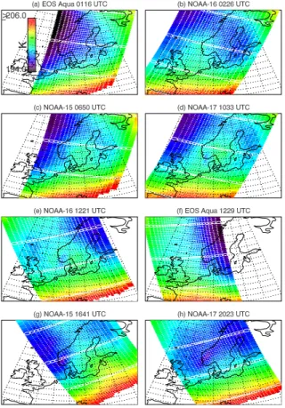
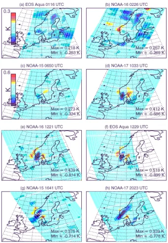
Figure2plots AMSU-A Channel 9 brightness temperatures T_B( ˆλ_j, ˆφ_j) acquired during the ascending and descending overpasses of Scandinavia by EOS Aqua, NOAA-15,

20

NOAA-16 and NOAA-17 on 14 January 2003. The maps are arranged in chronological order, with data plotted as color-coded elliptical footprint pixels with dimensions spec-ified by the Channel 9 radiance acquisition model ofEckermann and Wu (2006): see their Fig. 6.

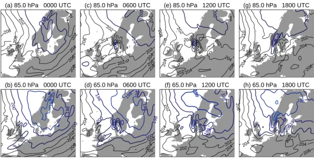
Figure3plots the 6-hourly ECMWF IFS analysis temperatures for 14 January 2003

25

at 85 hPa and 65 hPa, the approximate vertical range of the peak AMSU-A

(15)

ACPD

Full Screen / Esc

ing function responses at various beam positions (see Fig. 1b). Like the brightness temperatures, the analysis temperatures transition from warmer mid-latitude values to much colder values in and around Scandinavia.McCormack et al. (2004) showed that the very cold stratospheric temperatures over Scandinavia on 14 January 2003 were driven by adiabatic uplift from an anticyclonic upper-tropospheric ridge over Western

5

Europe and a weak wave-1 stratospheric disturbance that pushed the vortex core off the pole towards Scandinavia. These vortex disturbances presaged a minor strato-spheric warming, which split the vortex about a week later (McCormack et al.,2004) and shut off much of the early season PSC formation and ozone loss chemistry (Feng et al.,2005).

10

Despite gross similarites, variations in the brightness temperature maps from mea-surement to meamea-surement in Fig.2do not correlate obviously with the analysis temper-atures in Fig.3. Since adjacent AMSU-A measurements can be separated by an hour or less, the 6-hourly resolution of the ECMWF analysis temperatures is too coarse to investigate these variations systematically, and so we turn now to hourly temperature

15

fields from the NOGAPS-ALPHA runs.

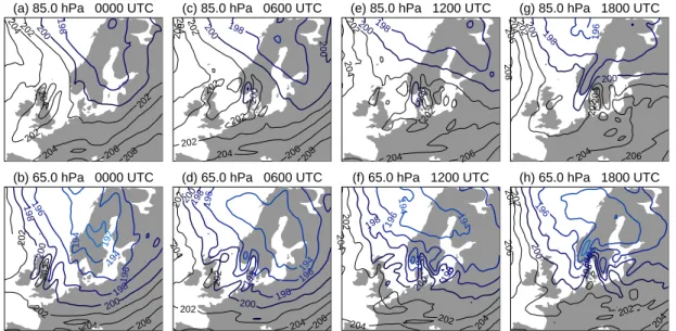
Figure4plots hindcast NOGAPS-ALPHA temperatures at times and altitudes corre-sponding to those plotted in Fig.3. The geographical structure and temporal evolution are very similar to the ECMWF analysis fields. In the “cold pool” regions, NOGAPS-ALPHA shows a cold bias of ∼1–2 K relative to the ECMWF analysis, which originates

20

mostly from the NAVDAS fields used for initialization (not shown), which have a 1–2 K cold bias relative to the ECMWF analysis in these cold-pool regions. Apart from this the comparison is very good, even down to details in the small-scale temperature oscil-lations over southern Scandinavia and Scotland, which we will focus on subsequently.

Next, we compute synthetic brightness temperature fields T_B

NWP( ˆλj, ˆφj) from these 25

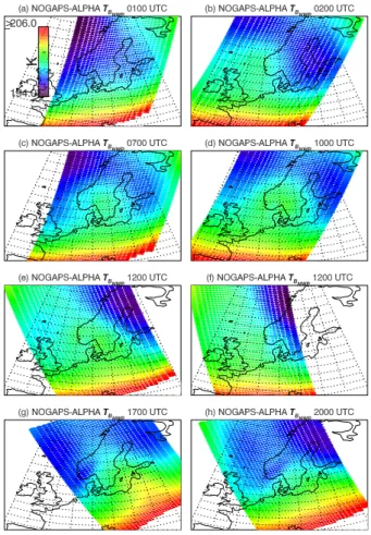
NOGAPS-ALPHA temperatures by evaluating Eq. (2) via the methods outlined in Sect. 3.2. For each AMSU-A measurement in Fig. 2, we evaluate Eq. (2) using the hourly NOGAPS-ALPHA temperature field closest in time to this satellite overpass. Results are plotted in Fig.5.

(16)

ACPD

Full Screen / Esc

Synthetic NOGAPS-ALPHA brightness temperatures in each panel of Fig. 5 com-pare very well in both magnitude and horizontal structure with the corresponding AMSU-A data in Fig. 2. This indicates that most of the panel-to-panel differences in Fig.2do not originate from biases among the various instruments deployed on dif-ferent satellite platforms. Rather, most of the variability comes from the limb effect,

5

which causes the far off-nadir measurements at the edges of the cross-track swaths to peak at ∼65 hPa, while those near-nadir measurements in the middle of the swath peak nearer 85 hPa (Goldberg et al.,2001;Eckermann and Wu,2006).

Thus, for example, the very cold brightness temperatures at 01:16 UTC to the west of Scandinavia in Figs. 2a and 5a can be understood in terms of far off-nadir

mea-10

surements at the edge of the swath that measure the compact core of cold 65 hPa temperatures in Fig.4b. The overpass 1 h later in Figs. 2b and5b measured warmer brightness temperatures here since it sampled this region with near-nadir beams which measured the significantly warmer 85 hPa temperatures in Fig.4a, while the off-nadir beams sampled the warmer 65 hPa temperatures located either side of this cold core

15

in Fig.4b.

The excellent reproduction of the measured brightness temperatures of Fig.2by this synthetic field in Fig.5governed by NWP model output gives us confidence that both our 3-D NWP hindcast temperature fields and the 3-D model weighting functions of Eckermann and Wu(2006) are sufficiently accurate to permit quantitative

intercompar-20

isons between the AMSU-A radiances and NWP temperature fields.

5 Gravity waves over Scandinavia on 14 January 2003

5.1 AMSU-A measurements

To isolate perturbations T_B0( ˆλ_j, ˆφ_j) from the raw brightness temperatures in Fig.2, we estimated a large horizontal-scale background field ¯T_B( ˆλ_j, ˆφ_j) using the following

algo-25

rithm.

(17)

ACPD

Full Screen / Esc

First, we performed 11-point (∼650 km) along-track smoothing of the radiances. These smoothed data were then fitted cross track for each scan using a least-squares sixth-order polynomial. These curves fitted both systematic cross-track trends in the ra-diances due to the limb effect and any instrumental biases (e.g.,Wu,2004;Eckermann and Wu,2006), as well as geophysical gradients produced by horizontal structure in

5

the temperature fields evident in Figs.2–5. These fitted data were then subjected to 5-point along-track smoothing to yield our final ¯T_B( ˆλ_j, ˆφ_j) field. The widths of these along-track averaging windows and the order of the polynominal fits were all tuned to give the best tradeoff between retaining as much long wavelength gravity wave struc-ture in the data as possible (aligned at any direction with respect to the scan axis),

10

while removing the background radiance structure evident in Fig.2 as completely as possible.

Perturbations were isolated by differencing at each measurement location, i.e.,

T_B0( ˆλ_j, ˆφ_j)= T_B( ˆλ_j, ˆφ_j) − ¯T_B( ˆλ_j, ˆφ_j). (3) We applied 3×3 point smoothing to these perturbation fields to suppress gridpoint

15

noise. Figure 6 plots maps of T_B0( ˆλ_j, ˆφ_j) extracted in this way from the correspond-ing raw radiances in Fig.2.

At ∼01:16 UTC and 02:26 UTC (panels a and b in Fig.6), the perturbation maps are essentially featureless. They show what appear to be small-amplitude artifacts from incomplete removal of background radiance structure, with peak amplitudes no larger

20

than ∼0.2–0.25 K. These values are in the range of the absolute AMSU-A noise floor values of ∼0.15–0.25 K (Mo,1996;Lambrigtsen,2003;Wu,2004;Eckermann and Wu, 2006). Thus there appears to be little or no wave-like structure imaged in the Channel 9 radiances over Scandinavia at these times.

At 06:50 UTC during a NOAA-15 overpass, we see in Fig.6c the first suggestions of

25

a resolved wave-like oscillation in the radiance perturbation maps over southern Scan-dinavia (note the change in color scale from ±0.3 K to ±0.6 K in the maps at this time). In the subsequent AMSU-A overpasses at 10:33 UTC, 12:21 UTC and 12:29 UTC, this

(18)

ACPD

Full Screen / Esc

oscillation grows in amplitude to a maximum absolute peak perturbation of ∼0.9 K in the 12:29 UTC measurement from Aqua. In the final two measurements at 16:41 UTC and 20:23 UTC, the amplitude of the oscillation weakens slightly but also changes hor-izontal structure, attaining a longer wavelength that is aligned differently and has a packet width that is noticeably more elongated in the along-phase direction.

5

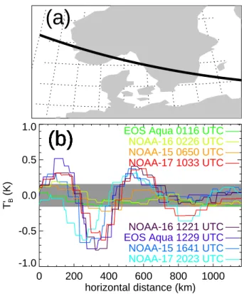
Figure7b plots brightness temperature perturbations along the horizontal trajectory in Fig. 7a for all 8 satellite overpasses. The 01:16 UTC curve lies below nominal noise floors, whereas the 02:26 UTC curve shows a peak at 100 km just above the nominal noise floor, indicating the initial presence of a weak wavelike oscillation. By 06:50 UTC an oscillation just above the noise is evident, which grows in amplitude while

10

maintaining the same wavelength and phase out to 12:29 UTC. The wavelength along this trajectory is ∼400–500 km, with slight increases by 16:41 UTC and 20:23 UTC. 5.2 NWP model fields

To isolate gravity wave perturbations from temperature fields generated by any one of our three NWP models, we use algorithms similar to those just described and applied

15

to the AMSU-A radiances. First, the three-dimensional temperature fields at a given model time were regridded vertically from their terrain-following model coordinates to a common high-resolution set of constant pressure surfaces to yield a 3-D tempera-ture field T ( ˆλ, ˆφ, p), where p is pressure. A background temperature field ¯T ( ˆλ, ˆφ, p)

was computed at each pressure level using a two-dimensional running average with a

20

width of ∼600–650 km. The precise width of this averaging window varied slightly from model to model, due to the different horizontal gridpoint resolutions ∆h and the result-ing integer number of gridpoints n needed to yield an averagresult-ing window n∆h within this 600–650 km range.

Perturbations were derived as

25

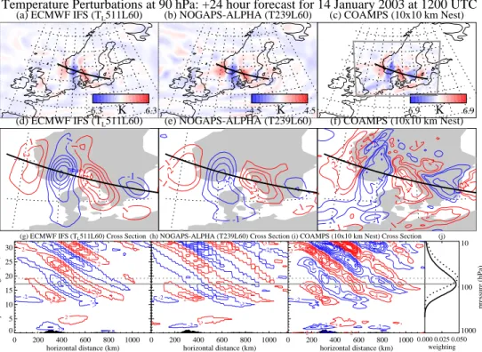
T0( ˆλ, ˆφ, p)= T (ˆλ, ˆφ, p) − ¯T ( ˆλ, ˆφ, p). (4) The upper two rows of Fig. 8 plot T0( ˆλ, ˆφ, p) fields at p=90 hPa from the three

(19)

ACPD

Full Screen / Esc

NWP models for+24 h forecasts initialized on 13 January 2003 at 12:00 UTC, valid at 12:00 UTC on 14 January. They show a mountain wave oscillation over southern Scan-dinavia with a geographical extent and phase structure very similar to the 12:00 UTC AMSU-A brightness temperature perturbations in Figs.6e and f.

The bottom panels in Fig. 8 plot altitude cross sections of the temperature fields

5

along the horizontal line plotted as the black curve in the panels above, which is the same trajectory used in Fig.7a. Each NWP model produces a similar-looking mountain wave temperature oscillation that grows in amplitude with altitude up to 10 hPa and beyond. The horizontal wavelength λ_his ∼400–500 km and the vertical wavelength λ_z is ∼12 km. The vertical range of the AMSU-A Channel 9 radiance acquisition through

10

this wave structure is depicted in Fig.8j using the 1-D vertical weighting functions for the near-nadir and far off-nadir scan angles from Fig.1b.

The most obvious difference among the three model fields is in the wave amplitudes. At 90 hPa, NOGAPS-ALPHA yields peak amplitudes T_PEAK∼4.5 K, ECMWF IFS yields

T_PEAK∼6 K, and COAMPS yields TPEAK∼7 K. This increasing trend in wave amplitudes

15

in consistent with increases in horizontal and vertical model resolution. Since the very smallest resolved scales in NWP models have little predictive skill (Lander and Hoskins, 1997;Davies and Brown,2001), NWP models smooth their gridscale orography (Der-ber et al., 1998; Webster et al., 2003) and apply scale-selective numerical damping to their prognostic fields (Skamarock, 2004) to suppress these smallest scales. As

20

a result, only at horizontal wavelengths greater than ∼6–10 times the minimum hor-izontal gridpoint resolution ∆h do waves appear in these models without significant attenuation of their amplitudes (Davies and Brown, 2001; Skamarock, 2004). Verti-cal resolution differences in Fig. 1a also contribute, though previous studies suggest they are secondary to horizontal resolution for gravity waves in the extratropics so long

25

as the vertical wavelength is sufficiently long (e.g., O’Sullivan and Dunkerton,1995; Hamilton et al.,1999).

Previous studies of Scandinavian stratospheric mountain waves in global and mesoscale models have shown that the resolved wave amplitudes in the global model

(20)

ACPD

Full Screen / Esc

can be underestimated by anywhere up to 50–80%. Hertzog et al. (2002) analyzed a stratospheric mountain wave over southern Scandinavia with a much shorter hor-izontal wavelength than here (λ_h∼200 km) and a slightly shorter vertical wavelength (λ_z∼10 km). While the estimated wave amplitude at ∼20 hPa was ∼9 K, the wave resolved in the ECMWF IFS T_L319L60 analyses had an amplitude of only 1.5 K and

5

the horizontal wavelength was overestimated. T_L319 corresponds to∆h of ∼60 km on the N160 reduced linear Gaussian grid. Since this λ_h∼200 km wave spans only 3–4 ECMWF gridpoints, it is not surprising that its amplitude was significantly underesti-mated (Skamarock,2004).

A mountain wave with wavelengths closer to the current example occurred over

10

northern Scandinavia on 26 January 2000: NWP forecasts yielded λ_h∼400 km,

λ_z∼10 km and TPEAK∼9 K at 30 hPa (D ¨ornbrack et al.,2002;Fueglistaler et al.,2003; Eckermann et al.,2006). Eckermann et al.(2006) found that the wave temperature am-plitude in the T_L319L60 ECMWF IFS forecast fields was 50% lower than in a mesoscale model run (see alsoFueglistaler et al.,2003). In this case, the horizontal wavelength

15

λ_h∼400 km spans around 6–7 ECMWF gridpoints, bringing it into the 6∆h–10∆h tran-sition zone whereSkamarock(2004) found that dynamics were resolved but somewhat suppressed in energy.

Our λ_h∼400–500 km mountain wave in the∆h=10 km nested COAMPS run spans 40–50 horizontal gridpoints. According to Skamarock (2004), COAMPS should

ac-20

curately simulate this wave, and thus for now we will take its simulated wave ampli-tude to represent the true wave ampliampli-tude. The T_L511 ECMWF spectral resolution corresponds to ∆h∼40 km on the reduced N256 linear Gaussian grid, making our

λ_h∼400–500 km wave a 10∆h oscillation in these fields and placing at the high end of

the 6–10∆h transition zone where amplitudes are not greatly suppressed (Skamarock,

25

2004). A comparison of Figs.8a and c bears this out. NOGAPS-ALPHA’s T239 spec-tral resolution yields a gridpoint resolution on the 720×360 quadratic Gaussian grid of ∼55 km at the equator, though the intrinsic resolution to zonal wavelengths is nearer 80 km at the equator. This places our wave in NOGAPS-ALPHA fields somewhere in

(21)

ACPD

Full Screen / Esc

the 5–9∆h range where we expect some significant amplitude underestimatation ( Ska-marock,2004;Eckermann et al.,2006), consistent with amplitude differences between Figs.8a and c

5.3 Suborbital validation of NWP model fields

For a more direct and objective assessment of the fidelity of the gravity waves in these

5

NWP fields, we now compare them directly to suborbital measurements of the lower stratosphere over southern Scandinavia on 14 January 2003.

5.3.1 Radiosonde

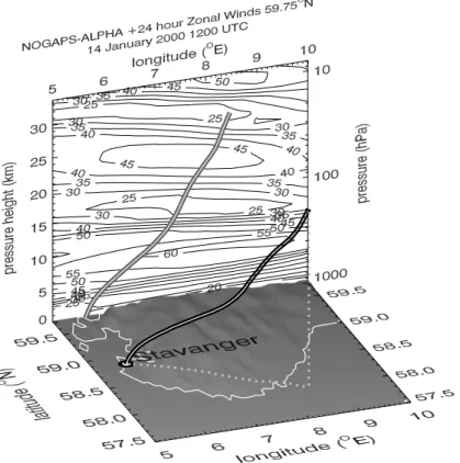
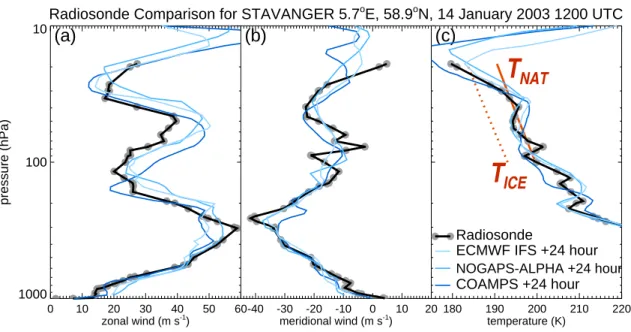
Figure 9 plots the estimated 3-D trajectory of the routine RS80 Vaisala radiosonde sounding made from Stavanger/Sola (58.86◦N, 5.65◦E) on 14 January 2003 at

10

12:00 UTC. The calculation uses the radiosonde horizontal winds from this ascent and assumes passive frictionless advection of the balloon as it ascends at a constant assumed velocity of 5 m s−1 (Lane et al.,2000). The inferred ground trajectory (dot-ted gray curve in Fig.9) takes this balloon through the regions of largest stratospheric gravity wave amplitudes evident in the NWP model fields in Fig.8. Assuming an ontime

15

12:00 UTC launch, we estimate the balloon reached 90 hPa just before 13:00 UTC. The contours in Fig.9show the NOGAPS-ALPHA+24 h (12:00 UTC) zonal winds at 59.75◦N. They reveal strong surface westerlies of ∼20 m s−1 that increase with height to a tropopause jet stream exceeding 60 m s−1, and a wave-induced horizontal velocity oscillation of around ±10 m s−1 in the stratosphere superimposed on mean

wester-20

lies of 30–40 m s−1. The strong westerly flow at all altitudes is consistent with surface forcing of quasi-stationary mountain waves and free propagation of those waves into the stratosphere (i.e., no critical level). The wave phase lines slope downward on pro-gressing eastward, as in the temperature cross sections in Figs.8g–i, consistent with a quasi-stationary mountain wave propagating upward and westward in this eastward

25

(22)

ACPD

Full Screen / Esc

Observational studies often assume that gravity wave fluctuations in radiosonde data can be interpreted as a purely vertical profile through the 3-D wave field directly above the launch site. Here, however, the strong westerlies advect the balloon substantial distances to the east. Figure9 shows rather clearly in this case that the radiosonde samples a significantly different wave structure along its oblique ascent trajectory than

5

the purely vertical profile directly above Stavanger, an issue highlighted in some pre-vious observational studies of mountain waves using radiosonde data (e.g.,Shutts et al.,1988;Lane et al.,2000). Thus our model-data comparison in Fig.10compares the radiosonde zonal winds U , meridional winds V and temperatures T with correspond-ing 12:00 UTC fields from the 3 NWP model runs that were sampled along the 3-D

10

radiosonde trajectory in Fig.9.

The NWP wind and temperature profiles in Fig.10are close to the radiosonde data at all altitudes. The stratospheric wave oscillation is most prominent in the zonal winds in Fig.10a. The model fields reproduce its amplitude and phase quite well, given the uncertainties in the actual balloon trajectory, model errors and slight time mismatches

15

between NWP fields and the radiosonde. Though the wave appears more weakly in the meridional wind and temperature profiles, the NWP fields match the amplitude and phase structure well in these profiles too.

The upper-level radiosonde temperatures in Fig. 10c are extremely cold. The fi-nal radiosonde measurement of 179.6 K near 19 hPa is only ∼1 K warmer than the

20

record low stratospheric radiosonde temperature of 178.6 K reported byD örnbrack et al. (1999) from 35 years of soundings from Sodankyl ä (67.4◦N, 26.7◦E) in northern Finland (though this record value was subsequently eclipsed in January 2001: seeKivi et al.,2001). Since Stavanger/Sola lies some 8.5◦equatorward of Sodankyl ä, this low temperature is unusual and ordinarily might be questioned given that it was the final

25

measurement acquired just prior to the balloon bursting. However, the NWP model profiles computed along its ascent trajectory in Fig.10c strongly suggest that the data here are reliable, and that these cold temperatures result from passage of the balloon through the cooling phase of a large-amplitude stratospheric mountain wave.

(23)

ACPD

Full Screen / Esc

5.3.2 NASA DC-8 flight

Red curves in Fig. 10c show that these very cold temperatures at 20 hPa lie below the frost point temperature T_ICE, which should cause type II (ice) PSCs to form here if nucleation material is present. Aerosol lidar data acquired from a NASA DC-8 flight on this day allow us to test this inference, and to validate the NWP model fields further.

5

During January 2003 the DC-8 was operating from Kiruna airport (67.8◦N, 20.3◦E) in northern Sweden, in support of NASA’s second SAGE III Ozone Loss and Vali-dation Experiment (SOLVE II; seeMcCormack et al.,2004). The cold synoptic strato-spheric conditions and stratostrato-spheric mountain wave activity over southern Scandinavia on 14 January 2003 were both forecast several days beforehand using ECMWF IFS

10

fields and the NRL Mountain Wave Forecast Model (MWFM), extending similar in-field wave forecasting efforts inaugurated for SOLVE during 1999–2000 and reported by Eckermann et al.(2006).

NAVDAS 925 hPa geopotential heights at 12:00 UTC in Fig. 11a show that the wave forcing on 14 January was driven by a compact polar low whose core moved

15

rapidly eastward across central Scandinavia, bringing with it strong surface westerly flow across the southern Scandinavian Mountains. The near-zero surface winds over central Scandinavia in the core of the low and weak surface easterlies across northern Scandinavia account for the confinement of the stratospheric wave activity to the south, since little mountain wave activity is forced over central Scandinavia, while any waves

20

generated to the north are absorbed at upper tropospheric critical levels as the flow transitions from surface easterlies to upper tropospheric and stratospheric westerlies.

The SOLVE II forecasts for 14 January predicted PSCs forming within the cold phases of mountain waves over southern Scandinavia. Based on this forecast guid-ance, a DC-8 flight from Kiruna was devised containing a southward leg to fly beneath

25

these forecast wave PSCs and profile them with onboard lidars. The final DC-8 flight track is plotted in blue in Fig.11a, with filled circles marking every 30 min along the flight segment from 06:00–09:30 UTC. The radiosonde trajectory from Fig.9is plotted

(24)

ACPD

Full Screen / Esc

in red. We see that the DC-8 flew beneath the cold 20 hPa stratospheric region sam-pled at the end of the radiosonde trajectory just after 07:00 UTC, some 5–6 h before the radiosonde sampled this region. From the AMSU-A data in Fig.6c, the mountain wave appeared to be present in this region at 07:00 UTC when the DC-8 arrived, but had a weaker amplitude than at the time of the radiosonde intercept at 12:00–13:00 UTC.

5

Figure 11b plots S₁₀₆₄ from the GSFC/LaRC lidar returns (see Sect. 2.2) from 06:00 UTC to 09:30 UTC, a flight segment marked with the thicker blue line in Fig.11a. Extensive PSC aerosol was measured in a number of thin tilted layers in the 20–26 km altitude range. Isolated yellow–red regions where S₁₀₆₄is ∼50–200 likely indicate ice (type II) PSCs.

10

Figure11c plots temperatures T ( ˆλ, ˆφ, Z_geo) from the NOGAPS-ALPHA+19 h hind-cast (valid at 07:00 UTC) along this DC-8 flight track. Here we have profiled the fields as a function of model geopotential height Z_georather than pressure height Z , to permit more direct comparison with the geometric altitude registration of the lidar data. The coldest temperature contours ≤190 K are color coded, and correlate impressively in

15

altitude and variation with flight time with the lidar data in the panel above. In particular the isolated region of large S₁₀₆₄ at 25 km at 07:00 UTC is colocated with a compact region of the coldest NOGAPS-ALPHA temperatures of ∼184 K, plotted as red con-tours. This 25 km altitude corresponds to pressures of ∼18–20 hPa (see grey contours in Fig. 11d). From Fig. 11a we see that this isolated type II PSC layer measured at

20

07:00 UTC in panel (b) occurs at the same geographical location intercepted 5–6 h later by the radiosonde, which measured very cold temperatures T <T_ICE in Fig. 10c that should form ice PSCs. Thus the radiosonde, lidar and NWP temperature data all cross-validate at this location.

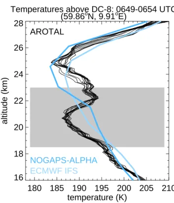
AROTAL Rayleigh temperature profiles are also available from this flight. However,

25

the presence of sunlight and PSC aerosol yielded noisy retrieved temperatures with large errors or data gaps within and below the PSC layers. Thus we focus on a 5 min flight interval starting at 06:49 UTC when S₁₀₆₄in Fig.11b is small at all altitudes just prior to the intercept of the ice PSC at ∼07:00 UTC. AROTAL temperatures for this

(25)

ACPD

Full Screen / Esc

period are plotted in Fig.12alongside the NOGAPS-ALPHA and ECMWF IFS temper-ature profile closest in time and location. The grey region in Fig.12 marks altitudes where PSC layers were observed earlier in the flight in Fig. 11b, and thus contain aerosol which can contaminate the retrieval. Indeed, the cold temperature “biteout” in the data at 21 km in Fig.12resembles the structure of the PSC-contaminated retrieved

5

Rayleigh temperature profile shown in Fig. 7 of Burris et al. (2002b). Thus we view AROTAL temperatures in this region as suspect. Above this grey strip (Z ≥23 km), we assume more PSC-free air that yields a more accurate retrieved temperature. Specif-ically, at 25 km the AROTAL temperatures drop to a minimum of ∼184 K, which again agrees well with the NOGAPS-ALPHA temperatures in Fig.11c and12and is

consis-10

tent with the ice PSC encountered minutes later at this altitude by the DC-8.

We speculated that the mountain wave perturbations produced the very cold 20 hPa temperatures in this region. To assess this, we split the NOGAPS-ALPHA temperature field into its component background field ¯T ( ˆλ, ˆφ, p) and perturbation field T0( ˆλ, ˆφ, p)

from Eq. (4), and plot each in Figs.11d and e, respectively, along the DC-8 flight track.

15

The background temperatures show a gently sloping layer of cold temperatures at 22– 24 km that explains a small part of the large-scale PSC tilting evident in the aerosol data, but little else. Clearly the omitted wave component produces most of the ob-served structure in these PSC layers. The perturbation temperatures in Fig.11e show that the ice PSC at 07:00 UTC is produced by a mountain wave-induced temperature

20

perturbation that cools this region by about 6–8 K. This then is clearly a mountain wave–induced ice PSC.

The minimum NOGAPS-ALPHA temperature in Figs.11c and 12of ∼184 K is at or just slightly above the 20 hPa frost point temperature shown in red in Fig.10c. That ice PSCs were measured here suggests that wave amplitudes were underestimated in the

25

NOGAPS-ALPHA run, consistent with our earlier inferences based on its T239L60 res-olution. To assess this, Fig.13a plots corresponding 07:00 UTC temperatures from the COAMPS run, which show a thicker layer of much colder temperatures at 07:00 UTC due to larger wave amplitudes in this higher resolution model.

(26)

ACPD

Full Screen / Esc

At 12:00–13:00 UTC when the radiosonde entered this region, the minimum 12:00 UTC NOGAPS-ALPHA temperature along the radiosonde trajectory in Fig.10c was ∼180 K, significantly colder than the 184 K in Fig.11c. This suggests that the wave in the NOGAPS-ALPHA run grew significantly in amplitude from 07:00 UTC to 12:00 UTC, consistent with what the AMSU-A data in Fig.6appear to show. To assess

5

this, Fig.13b plots corresponding NOGAPS-ALPHA temperatures along the DC-8 flight trajectory using the+24 h forecast fields, valid at 12:00 UTC. We see that the minimum temperatures are now 180 K, 4 K cooler than in Fig.11c, indicating a growth in peak wave amplitude of ∼4 K from 07:00 UTC to 12:00 UTC, and again consistent with the 179.2 K radiosonde temperature measured at 19 hPa in Fig.10c.

10

6 Brightness temperature perturbations from forward modeled NWP

tempera-ture fields

Having validated the NWP temperature fields against available suborbital data, we now insert these fields into Eq. (2) to derive anticipated AMSU-A Channel 9 brightness temperature perturbations, which we compare against the observed AMSU-A

pertur-15

bations. This represents our approach to validating the gravity wave signals in AMSU-A Channel 9 radiances.

6.1 Forward modeled NWP temperature perturbations

We begin with direct forward modeling of the NWP wave temperature perturbation fields T0( ˆλ, ˆφ, p) to yield a brightness temperature perturbation field

20 T_B0 NWP(Xj, Yj)= Z Z Z W_j(X − X_j, Y − Y_j, Z ) T0(X, Y, Z )d X d Y dZ. (5)

Similar calculations for idealized 3-D wave temperature oscillations were performed by Eckermann and Wu(2006).

(27)

ACPD

Full Screen / Esc

Our calculations here use the orbital scan data from the AMSU-A overpasses as out-lined in Sect.3.2. Final T_B0

NWP( ˆλj, ˆφj) maps incorporated the same 3×3 point smoothing

applied to the AMSU-A perturbations in Fig.6. Figure14 plots resulting T_B0

NWP( ˆλj, ˆφj)

fields for AMSU-A 12:21 UTC measurements from NOAA-16 (top row) and 12:29 UTC measurements from EOS Aqua (bottom row), based on 12:00 UTC (+24 h forecast)

5

T0( ˆλ, ˆφ, p) fields from ECMWF IFS, NOGAPS-ALPHA and COAMPS. The

correspond-ing AMSU-A data from Fig.6are reproduced in the right panels of Fig.14for compari-son.

The synthetic NWP T_B0

NWP( ˆλj, ˆφj) maps all show a wave oscillation over southern

Scandinavia that matches the AMSU-A data well in location, horizontal extent,

orien-10

tation and phase. In terms of amplitude, the ECMWF IFS amplitudes are close to the measured values. The NOGAPS-ALPHA amplitudes are smaller, consistent with ex-pected underprediction of wave amplitudes in these T239L60 runs, as discussed in Sect.5.2. The COAMPS amplitudes are fairly close to the EOS Aqua AMSU-A obser-vations, but somewhat larger than the NOAA-16 AMSU-A observations.

15

Indeed, despite using the same 12:00 UTC T0( ˆλ, ˆφ, p) fields, all the resulting T_B0

NWP( ˆλj, ˆφj) amplitudes in Fig. 14 are systematically larger for the NOAA-16 scan

pattern than for the EOS Aqua scan pattern. This is despite the fact that the lower orbit altitude of EOS-Aqua compared to NOAA-16 yields smaller horizontal footprints that should make EOS Aqua AMSU-A measurements slightly more sensitive to gravity

20

waves of a given scale than those on the NOAA satellites (Eckermann and Wu,2006). The smaller EOS Aqua T_B0

NWP( ˆλj, ˆφj) amplitudes in Fig. 14 arise due to the height

variation of the wave temperature amplitudes in the NWP models. As shown in the bot-tom row of Fig.8, the wave temperature amplitudes in all 3 models decrease between 80–90 hPa and 50–60 hPa. For example, the corresponding maximum ECMWF IFS

25

amplitude at 60 hPa is 4.8 K compared to the 6.3 K at 90 hPa in Fig.8a. The wave in the NOAA-16 12:21 UTC overpass data lies near the center of the scan pattern and so is observed by the near-nadir beams whose weighting functions peak near 80–90 hPa. Conversely, the wave is located towards the right edge of the EOS Aqua scan pattern,

(28)

ACPD

Full Screen / Esc

where it is observed by off-nadir beams which peak at higher altitudes (see Fig. 8j). The weaker NWP model temperature amplitudes at these higher altitudes lead to a weaker NWP brightness temperature perturbation for the EOS Aqua scan.

In contrast to the model fields, the observed AMSU-A perturbation amplitudes are slightly larger for the EOS Aqua overpass in Fig.14g than for the NOAA-16 overpass in

5

Fig.14d. This suggests that, while the NWP models have captured the wave structure and mean wave amplitudes quite well, the actual vertical variation in wave amplitudes over the 50–90 hPa range may have differed from the model predictions.

6.2 Perturbations isolated from forward modeled NWP temperatures

Next we perform more realistic forward modeling by using the raw NWP model

temper-10

ature fields to simulate a brightness temperature field T_B

NWP( ˆλj, ˆφj) using Eq. (2), as

in Fig.2. Then, we apply exactly the same data reduction algorithms to these bright-ness temperature fields that we applied to the AMSU-A brightbright-ness temperature data in Sect.5.1, first deriving a background field ¯T_B

NWP( ˆλj, ˆφj) and then, following Eq. (3),

computing perturbation fields

15

T_B0

NWP( ˆλj, ˆφj)= TBNWP( ˆλj, ˆφj) − ¯TBNWP( ˆλj, ˆφj). (6)

Finally, 3×3 point smoothing is applied to these perturbation fields. Differences be-tween perturbation fields calculated using this method and those calculated in Sect.6.1 provide some feel for how well the numerical data reduction methods in Sect.5.1 iso-late gravity wave perturbations from raw AMSU-A radiances.

20

Figure 15 plots NWP perturbation brightness temperatures calculated using this method for the same set of 12:00 UTC fields and AMSU-A scans shown in Fig. 14. Oscillatory structure that closely resembles the measurements (panels d and g) is re-produced in all the NWP-based radiance fields over southern Scandinavia. On com-paring with corresponding panels in Fig.14, we see that T_B0

NWP( ˆλj, ˆφj) amplitudes here 25

are ∼10–25% smaller. Thus, wave perturbations are isolated well using these data 2029

(29)

ACPD

Full Screen / Esc

reduction procedures, being only slightly suppressed in amplitude. ECMWF IFS ampli-tudes in Fig.15are slightly smaller than the measured values, and NOGAPS-ALPHA amplitudes are significantly smaller at the negative (cold) wave phase. COAMPS am-plitudes are very similar to the EOS Aqua observations, but slightly larger than the NOAA-16 observations. More precise comparisons with data are provided shortly.

5

Figure16plots T_B0

NWP( ˆλj, ˆφj) maps based on NOGAPS-ALPHA temperature fields at

times closest to the corresponding measurements from all 8 AMSU-A overpasses in Fig. 6. Many aspects of the measurements in Fig. 6 are reproduced in Fig. 16. For example, at 01:00–02:00 UTC the perturbation maps look very similar despite show-ing no obvious wave perturbations over southern Scandinavia and small amplitudes

10

near nominal AMSU-A noise floors of ∼0.15–0.2 K. At ∼07:00 UTC the wave appears weakly overly southern Scandinavia, then grows in amplitude during the period 07:00– 12:00 UTC. The horizontal wavelength, geographical extent, orientation and phase all agree well with observed fluctuations in Fig. 6. At 17:00 UTC and 20:00 UTC the wave phase fronts are rotated clockwise compared to earlier times, the packet width is

15

broader, the wavelength is longer, and the oscillation is dominated by a large-amplitude cold phase that extends farther northward and southward: all these features are seen in the observed maps in Figs.6g and h. The main differences are in the amplitudes. For the first 6 panels, the NOGAPS-ALPHA brightness temperature amplitudes in Fig.16 are smaller than those observed in Fig.6. Whereas the largest observed perturbation

20

amplitudes occur at ∼12:00 UTC in Fig. 6, the largest NOGAPS-ALPHA brightness temperature amplitudes in Fig.16occur at 17:00 UTC and 20:00 UTC. This is due (at least in part) to the longer horizontal wavelength at these later times (see, e.g., Fig.7b), which NOGAPS-ALPHA can explicitly simulate at T239L60 with less amplitude attenu-ation (Skamarock,2004).

25

Since the T239L60 NOGAPS-ALPHA runs underestimate this wave’s amplitude, we repeated these calculations using the hourly COAMPS fields. However, the regional COAMPS domain complicates these calculations. Specifically, when the numerical extraction methods used for AMSU-A data are applied to model brightness