HAL Id: hal-00331109
https://hal.archives-ouvertes.fr/hal-00331109
Submitted on 15 Oct 2008
HAL is a multi-disciplinary open access
archive for the deposit and dissemination of
sci-entific research documents, whether they are
pub-lished or not. The documents may come from
teaching and research institutions in France or
abroad, or from public or private research centers.
L’archive ouverte pluridisciplinaire HAL, est
destinée au dépôt et à la diffusion de documents
scientifiques de niveau recherche, publiés ou non,
émanant des établissements d’enseignement et de
recherche français ou étrangers, des laboratoires
publics ou privés.
data
S. K. Kravtsov, W. K. Dewar, M. Ghil, P. S. Berloff, J. C. Mcwilliams
To cite this version:
S. K. Kravtsov, W. K. Dewar, M. Ghil, P. S. Berloff, J. C. Mcwilliams. North Atlantic climate
variability in coupled models and data. Nonlinear Processes in Geophysics, European Geosciences
Union (EGU), 2008, 15 (1), pp.13-24. �hal-00331109�
www.nonlin-processes-geophys.net/15/13/2008/ © Author(s) 2008. This work is licensed under a Creative Commons License.
Nonlinear Processes
in Geophysics
North Atlantic climate variability in coupled models and data
S. K. Kravtsov1,2, W. K. Dewar3, M. Ghil2,4, P. S. Berloff5,6, and J. C. McWilliams2
1Department of Mathematical Sciences, University of Wisconsin-Milwaukee, P. O. Box 413, Milwaukee, WI 53201, USA 2Dept. of Atmospheric and Oceanic Sciences, & Institute of Geophysics and Planetary Physics, University of California at
Los Angeles, Los Angeles, CA 90095–1565, USA
3Dept. of Oceanography, Florida State University, Tallahassee, FL, 32306, USA
4D´epartement Terre-Atmosph`ere-Oc´ean, & Laboratoire de M´et´eorologie Dynamique (CNRS and IPSL), Ecole Normale
Sup´erieure, F-75231 Paris Cedex 05, France
5Dept. of Physical Oceanography, Woods Hole Oceanographic Institution, Woods Hole, MA 02543, USA 6DAMTP, University of Cambridge, Cambridge, UK
Received: 23 May 2007 – Revised: 4 October 2007 – Accepted: 6 December 2007 – Published: 18 January 2008
Abstract. We show that the observed zonally averaged jet
in the Northern Hemisphere atmosphere exhibits two spa-tial patterns with broadband variability in the decadal and inter-decadal range; these patterns are consistent with an im-portant role of local, mid-latitude ocean–atmosphere cou-pling. A key aspect of this behaviour is the fundamentally nonlinear bi-stability of the atmospheric jet’s latitudinal po-sition, which enables relatively small sea-surface temper-ature anomalies associated with ocean processes to affect the large-scale atmospheric winds. The wind anomalies in-duce, in turn, complex three-dimensional anomalies in the ocean’s main thermocline; in particular, they may be respon-sible for recently reported cooling of the upper ocean. Both observed modes of variability, decadal and inter-decadal, have been found in our intermediate climate models. One mode resembles North Atlantic tri-polar sea-surface temper-ature (SST) patterns described elsewhere. The other mode, with mono-polar SST pattern, is novel; its key aspects in-clude interaction of oceanic turbulence with the large-scale oceanic flow. To the extent these anomalies exist, the inter-pretation of observed climate variability in terms of natural and human-induced changes will be affected. Coupled mid-latitude ocean-atmosphere modes do, however, suggest some degree of predictability is possible.
1 Introduction
Coupled ocean–atmosphere dynamics is rich in scientific challenges, as well as socio-economic implications. A well-known example of coupled variability is the El Ni˜no/ Southern Oscillation (ENSO) phenomenon – a seasonal and inter-annual climate event with substantial atmospheric and
Correspondence to: S. K. Kravtsov
oceanic manifestations in the Tropical Pacific and global im-pacts on temperatures and precipitation. Potentially cou-pled phenomena in the mid-latitudes may include the North Atlantic Oscillation (NAO: Hurrell, 1995) and the Pacific Decadal Oscillation (PDO: Mantua et al., 1997). These two oscillations exhibit considerable power at decadal and lower frequencies and also affect the climate of adjacent continen-tal areas. We present modelling and observational evidence that some of this decadal-to-inter-decadal power arises as a result of highly nonlinear, mid-latitude coupled modes and hence might exhibit some degree of predictability.
NAO and PDO spatial patterns appear in atmosphere-only general circulation models (AGCMs) subject to climatologi-cal sea-surface temperatures (SST) (Robertson, 2001), while AGCM sensitivity of these patterns to variable SST is model dependent (Saravanan, 1998; Rodwell et al., 1999; Mehta et al., 2000; Robertson, 2001); coupled general circulation models (CGCMs), in turn, show differing degrees of locally coupled behaviour (Latif et al., 1996; Pierce et al., 2001; Robertson, 2001). We investigate here atmospheric patterns reminiscent of the NAO, as well as PDO, and show evidence of coupling in the Atlantic sector.
Deser and Blackmon (1993) presented observational evi-dence for a 9–12-yr NAO-like signal in the North Atlantic atmosphere; they associated this signal with a tripolar SST pattern, whose amplitude may be controlled by a positive ocean–atmosphere feedback. Other analyses have linked a longer, 30–35-yr signal in co-varying North Atlantic sea-level pressure (SLP) and SST fields with coupled dynamics (Levitus, 1989; Kushnir, 1994). More recently, a spectral peak in North Atlantic SLP and in an ad-hoc North Atlantic SST index provided support for coupled ocean–atmosphere variability at a period of roughly 20 yr (Czaja and Marshall, 2001).
Marshall et al. (2001) compiled a thorough review of observational, modeling, and theoretical studies of
Fig. 1. Atmospheric bimodality in atmospheric quasi-geostrophic (QG) model and observations: (a) Results from the QG channel model show zonally averaged jet latitudes versus atmospheric bot-tom drag. The regime of “observed” values as taken from GCMs appear on the x-axis. Note the bifurcation at 6 days beyond which the jet exhibits bimodality. In an uncoupled simulation, transitions between the sites are accurately modelled by a white-noise pro-cess. In a coupled model, these transitions exhibit a preferred time scale controlled by ocean processes. (b) A phase space plot of the principal components of the first two EOFs of the zonally averaged zonal wind in the Northern Hemisphere. Departures from a Gaus-sian distribution are indicative of atmospheric bimodality. Regions where such departures are significant at the 95% confidence level are shaded. The two regions containing the statistically significant PDF maxima are outlined and labelled “A” and “B”. The 250-hPa spatial patterns associated with the regimes appear in (c) and (d). For (c) and (d), contour interval CI=20 m, yellow/green ∼0 m.
climate variability in the Atlantic sector. These authors have presented evidence for a global significance of the Atlantic-based climate modes, comparable to that of ENSO. A brief, but fairly comprehensive account of existing theories for the climate variability in the Indo-Pacific region can be found in Power and Colman (2006). In a nutshell, natural cli-mate variability in mid-latitudes has been attributed to atmo-spheric, oceanic, or coupled ocean–atmosphere processes, with the relative contribution of each type of process still be-ing unknown. Conceptual explanations of extra-tropical cli-mate modes range from Hasselmann’s (1976) passive ocean scenario, to linear theories emphasizing oceanic dynamical adjustment (Marshall et al., 2000), to explanations involving nonlinear mechanisms (see Kravtsov et al., 2007a for a more detailed review). Air-sea feedbacks can potentially modify decadal modes rooted in the ocean dynamics, or play a more substantial role in mechanisms that do not operate in the ab-sence of ocean-atmosphere coupling.
A key ingredient of the coupling mechanism illustrated in the present paper is the bi-stability of mid-latitude
atmospheric jets, i.e. the tendency for the zonally aver-aged jet to be found, preferentially and persistently, in two separate latitude ranges. Koo et al. (2002) adduced strong evidence for such behaviour in the Southern Hemisphere’s zonally averaged jet. Kravtsov et al. (2006a) used the NCEP– NCAR reanalysis data (Kalnay et al., 1996) to highlight two regimes in the Northern Hemisphere’s zonally averaged jet. The regimes were defined in the phase space of the two lead-ing Empirical Orthogonal Functions (EOFs) of the vertically and zonally averaged zonal wind (Fig. 1b). The zonal-wind regime composites (not shown) defined as averages over the days belonging to the subjectively chosen ellipse A and cir-cle B in Fig. 1b show that these regimes consist mainly of meridional shifts relative to the climatological jet position. The composite maps of these regimes’ 250-hPa height fields (Fig. 1c, d) also show considerable zonality and both have ex-trema straddling the latitudinal location of the climatological mid-latitude jet; this means, due to geostrophy, that Regime A/B has the jet displaced poleward/equatorward of its time-mean latitudinal position. These regimes resemble opposite phases of the Arctic Oscillation (Deser, 2000) and have an equivalent barotropic vertical structure (not shown).
An idealized atmospheric circulation model set up in a quasi-geostrophic (QG) two-layer channel configuration (Kravtsov et al., 2005) produces a similar bi-stability, with the preferred latitudes of the maximum zonally averaged wind depending on the bottom drag parameter. Strongly damped solutions have single preferred latitude, while more realistic, weaker damping yields two distinct solutions (Fig. 1a).
The transitions between the preferred latitudes in the above atmosphere-only setting are random. Coupling to a one-basin, three-layer QG ocean circulation model (Kravtsov et al., 2006b, 2007a), however, introduces an apparent regu-larity into these transitions by affecting the occupation fre-quency of the high-latitude and low-latitude atmospheric regimes on a decadal time scale. The two jet states gen-erate differing wind-driven ocean circulations that, in turn, produce different SST fields and thus differing air–sea heat exchanges. The heat flux from one of these two states modi-fies the jet transition behaviour and thus favours development of the other ocean state1. Suppose, for example, that the occupation frequency of the atmospheric low-latitude state increases, so that atmospheric jet spends more time at lat-itudes lower than the latitude of climatological jet. This will eventually force the relocation of the oceanic eastward jet (“Gulf Stream”) toward lower latitudes, but this happens not momentarily, but with a lag of a few years, because of
1Kravtsov et al. (2006b) force the atmospheric QG channel
model coupled to oceanic mixed layer by oceanic QG interior states keyed to the phases of the decadal oscillation. These experiments show that the when the oceanic jet is located poleward of its time-mean position, the atmosphere tends to spend more time in low-latitude regime, and vice versa.
the Gulf Stream’s eddy inertia associated with rectification process (Berloff, 2005; Berloff et al., 2007b), that is, the driving of the Gulf Stream extension by the eddies swept downstream by that same current. After this adjustment is complete, the ocean–atmosphere heat fluxes induce more fre-quent transitions to the high-latitude state, thus starting the opposite swing of the cycle. The period of the oscillation in the damped stochastically excited delayed oscillator such as the one described here is typically 3–4 times the lag value, depending on how strongly damped the oscillation is rela-tive to the intensity of the stochastic driving (Kravtsov et al., 2007b). Indeed, atmospheric and oceanic spectra from the coupled runs show statistically significant peaks in the inter-decadal range, while eddy activity in the ocean is critical to establishing the spectral peaks: they disappear in lower-resolution coupled runs with larger oceanic viscosities.
The inquiry pursued in the present paper builds upon these idealized modelling and observational results to argue for a link between relatively fast nonlinear atmospheric dynam-ics manifested through bi-stability of the atmospheric jet latitudinal position, and decadal-to-inter-decadal time scale climate variability. In particular, we identify, in Sect. 2, multi-year lag correlations between the frequencies of oc-currence of two anomalously persistent atmospheric states (or regimes) on one hand, and the sea-surface temperature on the other hand. These correlations are indicative of pos-sible presence of decadal and multi-decadal coupled climate modes.
One of these modes, characterized by an inter-decadal time scale and largely mono-polar SST pattern in the mid-latitude North Atlantic is reminiscent of the coupled mode described by Kravtsov et al. (2006b, 2007a); these similari-ties are discussed in Sect. 3. We also find, in Sect. 4, a sig-nature of this mode in the long-term co-variability of the at-mospheric regimes and upper-ocean heat content (Levitus et al., 2005; Lyman et al., 2006), and confirm the correspond-ing phase relations in our coupled QG model, thus addcorrespond-ing additional weight to our hypothesis that the dynamics of the observed multi-decadal mode may be captured correctly by the QG climate metaphor Sect. 3).
In Sect. 3, we also examine another mode, which may be substantially modified by mid-latitude ocean–atmosphere coupling. This mode exhibits a tri-polar North Atlantic SST pattern and a decadal time scale. We emphasize here, once again, the apparent effect of SST anomalies associated with this mode onto the occurrence frequency of one of the at-mospheric preferred regimes, which enables the atat-mospheric flow to be nonlinearly sensitive to slow oceanic evolution. To capture this mode turned out to require a relatively high vertical resolution (15-level) primitive-equation (PE) oceanic model (Kravtsov and Ghil, 2004) coupled, once again, to the QG atmosphere of Kravtsov et al. (2005).
The two modes identified in observations thus appear to be governed by distinctive dynamical mechanisms, as suggested by our idealized modelling. In Sect. 5, we summarize the
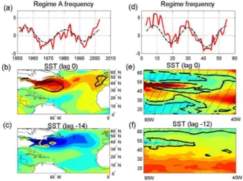
Fig. 2. Spatiotemporal patterns associated with Regime A of Fig. 1, in observations and all-QG coupled model: (a, b, c) observational features based on 55 years of reanalysis; and (d, e, f) coupled quasi-geostrophic model features based on the 700-yr simulation. (a, d) Time series of regime frequency occurrence, with abscissa in years and ordinate in regime days per winter; dashed lines in both plots represent the leading-pair SSA reconstruction. (b, c) and (e, f) Op-posite phases of the SST pattern from the data (left panels) and from the wind-driven ocean model (right panels), regressed onto the regime time series in Fig. 1a and d, respectively. For panels (b), (c), (e) and (f), CI=0.05◦C, values greater than (less than) 0.2◦C (−0.2◦C) shown by dark red (dark blue); yellow/green ∼0◦C. Area with values statistically significant at the 95% level are hatched.
evidence presented here in support of mid-latitude coupled dynamics, while emphasizing the controversial aspects of our approach. These include bi-stability and bimodality of the atmospheric jet and the use of QG models to study coupled dynamics. Avenues for the future research are outlined. Fi-nally, Appendix A describes spectral analyses we employed to identify periodicities in the time series considered, while Appendix B deals with the non-parametric method used to address the statistical significance of the patterns associated with our climate modes.
2 Atmospheric regimes and (multi-)decadal climate modes
The coupled QG climate model results summarized in Sect. 1 motivated our examination of the atmospheric jet transitions between the two regimes shown in Fig. 1 according to the 55 yr of NCEP-NCAR reanalysis (December 1948–March 2003). Specifically, we have counted the number of days spent in either regime during the winter months for each of the years. Ten-year running means of linearly de-trended occupation frequency of the two regimes appear in Fig. 2a for Regime A and in Fig. 3a for Regime B. Regime A ex-hibits fluctuations with time scales of 20–30 yr and Regime B of 10–15 yr; see Figs. 2b, c and 3b, c. The statistical
Fig. 3. Same as Fig. 2, but for 55 yr of reanalysis for Regime B and 4000-yr simulation of the buoyancy-driven ocean model.
significance of these time scales, especially the former, is suspect, because the record is only 55-yr long. However, the Singular Spectrum Analysis (SSA: Ghil et al., 2002) con-firms the presence of the oscillations in both regimes’ time series, with periods of 25 and 12 yr, respectively (see Ap-pendix A).
We have regressed the SST anomaly record at various tem-poral lags against the time series in Figs. 2a and 3a to visu-alize the ocean patterns correlated with the jet shifts. The Atlantic-sector SST signals appear in the left-hand panels (b) and (c) of Figs. 2 and 3. The regions of largest SST anomaly for both cases are found in the vicinity of the Gulf Stream; these anomalies are significant at the 95% confi-dence level, as determined by a non-parametric Monte-Carlo technique (Vautard et al., 1990; see Appendix B). In this technique, regime occurrences are shuffled and then averaged over winters to produce surrogate time series of occurrence frequency; the SST anomaly record is then regressed upon the time series so obtained.
The SST pattern of Regime A is dominantly mono-polar, with the maximum anomaly centred on the Gulf Stream axis (Fig. 2b, c). In contrast, SST anomalies for Regime B are tri-polar, essentially sharing central lobes with Regime A, but possessing lobes of the opposite sign to the north and south. A reversal of the patterns is found at lags of −14 yr (10 yr) for Regime A and −7 yr (5 yr) for Regime B; the patterns at positive lags are not shown. These lags are consistent with the inferred spectral peaks of the time series in Fig. 6a, b (see Appendix A), and with the associated broadband variability of Regimes A and B, respectively.
Finally, we note that statistically significant SST signals associated with both regime time series also appear in the Pacific basin (not shown). However, the location of these sig-nals is in the mid-Pacific, in contrast to the western-boundary intensified patterns of the Atlantic Ocean. The latter
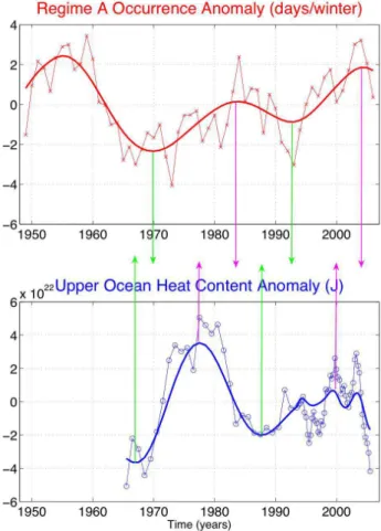
pat-Fig. 4. Atmospheric Regime A occurrence and upper-ocean heat content variability in the observed data. Upper panel: same as in Fig. 2a, but updated using the data up to 2006: light line with x-symbols is the original data, while heavy line is an SSA reconstruc-tion of the leading 25-yr mode. Lower panel: linearly detrended upper-ocean heat content (Levitus et al., 2005; Lyman et al., 2006): light line with circles is the original data; heavy line – smoothed version of the data. The green and magenta arrows mark a dis-tinctive phase relationship between the regime A occurrence and upper-ocean heat content variability.
terns are more likely caused by either oceanic or coupled ocean–atmosphere processes, rather than by surface atmo-spheric forcing. We thus speculate that the source of reg-ularity of the climate signals considered here comes from the North Atlantic ocean modes coupled to a bi-stable atmo-spheric jet, while the SST anomalies in the Pacific are sec-ondary, induced by the anomalous atmosphere–ocean heat fluxes associated with shifting of the atmospheric jet.
3 Comparison with idealized models
We have applied statistical analyses similar to those above to two intermediate coupled models (ICMs), both of which used an identical atmospheric component characterized by a bi-stability of the atmospheric jet position (Kravtsov et al., 2005), but distinct ocean components (see Sect. 1).
Fig. 5. Same as in Fig. 4, but for an arbitrary 55-yr-long portion of the all-QG coupled model; results based on the full 700-yr time series are analogous. The quantities plotted in both panels are di-mensionless, which is achieved by dividing the original time series by their respective standard deviation.
3.1 Results from all-QG coupled ocean–atmosphere model Results from a 700-yr run of the all-QG coupled model (Kravtsov et al., 2006b, 2007a) that has, in addition to the QG atmospheric component, a QG ocean component on an eddy-permitting mesh, with a resolution of km by 10-km and horizontal viscosity of 200 m2/s, appear in the right-hand panels of Fig. 2. The ocean model has three layers in the vertical and is set up in a rectangular basin of the size 5120×5600 km on a mid-latitude beta-plane. This configu-ration mimics, in an idealized fashion, the coupled ocean– atmosphere system comprised of the North Atlantic basin and the mid-latitude atmosphere above it and extending fur-ther up- and downstream. The atmospheric and oceanic model components are coupled via a simple ocean mixed-layer model with a diagnostic momentum closure and non-linear sea-surface temperature (SST) advection. Further de-tails of the all-QG coupled model can be found in Kravtsov et al. (2007a).
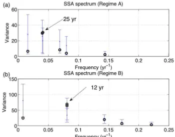
Fig. 6. Monte Carlo SSA spectra of the time series in Figs. 2a and 3a of the main text: (a) Regime A; and (b) Regime B. Error bars represent the 95% confidence interval associated with a red-noise null hypothesis.
Figure 2d shows the occurrence frequency anomaly of Regime A. The peak-to-peak amplitude of the regime-occurrence anomalies in the observations and in the model is surprisingly close, with ±4 days/winter for the observations and ±5 days/winter for the model. SSA analysis of the model time series in Fig. 2d identifies a statistically significant 25-yr oscillation, which matches the observed time scale. A re-gression analysis of the model SST anomalies against this time series yields the dominant time scale of 24 yr, given by anomalies of opposite sign for lags separated by 12 yr (see panels e and f); this time scale, in turn, is entirely consistent with the SSA results.
The patterns of SST variability that emerge from the model exhibit features that are broadly comparable to the ob-served, when taking into account the simplified model do-main. Specifically, the decadal scale variability in the cou-pled QG model is dominated by a local extremum in the vicinity of the separated Gulf Stream. This compares very well with the SST anomalies from the observations. It is known from the coupled QG model experimentation that these anomalies represent the effects of a waxing and waning Gulf Stream recirculation, itself maintained by the mesoscale variability of the unstable Gulf Stream.
The similarities between the left-hand panels (observa-tions) and right-hand panels (model) provide evidence for the mechanisms captured by this coupled QG model contributing to North Atlantic climate variability.
3.2 Results from PE–QG coupled ocean–atmosphere model
In contrast, the higher-frequency variability of Regime B is associated with the familiar tri-pole pattern seen in the left-hand panels of Fig. 3. This mode is not found in our cou-pled QG model. Here we examine the possibility that this decadal variability is associated with the bi-stability of atmo-spheric jet position coupled to fully three-dimensional wind-/buoyancy-driven upper ocean current anomalies.
To test this hypothesis, we have coupled a coarse-resolution, high-viscosity, primitive-equation (PE) compo-nent (Kravtsov and Ghil, 2004) to the same bimodal atmo-spheric model. In contrast to quasi-2D QG model, which only considers small perturbation to specified basic strat-ification, the PE formulation allows explicit modelling of large-scale convection processes characterized by displace-ments of the isopycnals much exceeding those assumed in the QG scaling. The details of the coupling are straightfor-ward. As the primitive equation model computes an SST automatically, heat exchange with the atmosphere proceeds as in the coupled quasi-geostrophic model. In addition, the primitive equation model accepts momentum flux at the top boundary as provided by the atmospheric channel QG model. The ocean model uses a coarse 400-km by 400-km resolution in the horizontal and 15 vertical levels. Horizontal viscosity levels are sufficiently high (1000 m2/s), so that the ocean is in a non-turbulent state.
A 4000-yr record was generated from this coupled model and the regime transitions were counted. Anomalies of the occurrence of Regime B exhibit low-frequency variability as appears in Fig. 3d. Again, the peak-to-peak amplitude of the model anomalies agrees well with that of the observations, both being of about ±10 days/winter.
The SSA analysis of this time series (see Appendix A) yields an 11-yr period, consistent with the lagged regression of model SST anomalies onto the regime time series (panels e and f), since the reversal in the anomaly pattern here occurs at time lags of −1 yr and −6 yr. This also compares well with the observed 12-yr period. The model SST anomaly fields are tri-polar (Fig. 3e, f), with the central lobe located over the mid-ocean eastward jet, which is also characteristic of the observed SST anomaly fields (Fig. 3b, c). These simi-larities between the modelled and observed decadal variabil-ity patterns suggest that some of this variabilvariabil-ity can be ex-plained, at least in part, by dynamical mechanisms captured by this coupled model, whose ocean component includes ex-plicit buoyancy effects.
4 Inter-decadal variability of the upper-ocean heat con-tent
The decadal-to-inter-decadal periods discussed in the previ-ous section suggest dynamical roles for oceanic processes in
these modes. The oceanic heat content is an important indi-cator of such a long-term oceanic variability. The latter vari-ability is dominated by that of the upper-ocean (top 700 m) heat content (Levitus et al., 2005; Lyman et al., 2006). Here we examine the time series of the upper-ocean heat content in relation to the Regime A occurrence frequency, for ob-servations (Fig. 4) and the all-QG coupled climate model (Fig. 5). The observed heat content has been linearly de-trended; causes of that trend are unclear, but do include an-thropogenic effects.
The upper panel of Fig. 4 shows the time series of the Regime A occurrence frequency, which is an updated version (1948–2006) of that shown in Fig. 2a. The upper-ocean heat content time series is plotted in the lower panel. This time se-ries leads the regime occurrences by a few years, meaning the two time series are roughly in quadrature, given the 20–25-yr time scale of the implied oscillatory signal. Such a distinctive phase relationship between the oceanic and atmospheric time series provides additional support that the coupled dynamics may be responsible for this behaviour, since it implies that the atmosphere is indeed affected by the ocean-induced SST anomalies on decadal time scales.
We have argued that the dynamical mechanism underlying the observed 20–25-yr oscillation is captured by our ideal-ized all-QG coupled climate model. Should this be the case, the phase relationship between the upper-ocean heat content and regime occurrence frequency in the model should repro-duce that observed. Figure 5 is an analogue of Fig. 4 based on data produced by the all-QG coupled model. The oceanic heat content is computed over the whole area of the model domain. For the purposes of direct comparison between the two figures, we plot in Fig. 5 an arbitrary 55-yr-long segment of the 700-yr-long coupled model run; the results based on the full 700-yr simulation are analogous. The SSA analy-sis of the upper-ocean heat content time series (not shown) confirms that this time series possesses a statistically signifi-cant spectral peak in the 20–25-yr range, consistent with the corresponding peak in the regime occurrence frequency (see Appendix A and Fig. 7).
The heavy solid lines in the upper and lower panels of Fig. 5 show the SSA reconstruction of this oscillation, based on single-channel SSA analysis of the regime occurrence and upper-ocean heat content time series, respectively. The phase relationship between the oceanic and atmospheric quantities in the model is analogous to that observed, with the upper-ocean heat content generally leading the regime occurrences by a few years. However, for the particular segment dis-played in Fig. 5, the phase difference drifts with time, in-creasing from the value of 5 yr in the beginning of the seg-ment, to the value of 10 yr at the end. Such a drift is indica-tive of a broadband nature of the oscillation under considera-tion. The phase relationship between two time series are bet-ter captured by a multi-channel version of the SSA analysis (M-SSA), which explicitly takes into account multi-year lag correlations between the time series of regime occurrences
and upper-ocean heat content. The M-SSA reconstruction of the 20–30-yr oscillatory signal (not shown) considerably reduces the phase drift between the two time series and re-covers the observational result of the in-quadrature phase relationship between them. The oceanic heat content vari-ance explained by the heat content component of the multi-channel SSA reconstruction (done on combined annual heat content and regime occurrence frequency time series over the 700-yr period) is roughly 40% of the total heat content vari-ance. The heat content’s spatial pattern associated with this mode is dominated by the anomalies in the region of oceanic eastward jet.
In summary, the combined observational and idealized modelling evidence suggests that the inter-decadal oscilla-tion characterized by a mono-polar SST signal in the mid-latitude North Atlantic Ocean is governed by coupled ocean– atmosphere dynamics.
5 Summary and discussion
We have presented here two modes of coupled climate vari-ability that both involve long-term variations in the occur-rence frequency of the two anomalously persistent zonal-jet regimes, which we called A and B (see Fig. 1). One of the modes, associated with Regime A, has a predominantly mono-polar SST pattern (Fig. 2) and a period of 25 yr; it is characterized by a distinctive phase relationship between the regime occurrences and upper-ocean heat content (Figs. 4 and 5). Modelling results show that this mode depends on ocean eddy activity, and is closely related to wind-driven cir-culation variability. The other mode is associated with at-mospheric Regime B, and reflects co-variability of the three-dimensional upper-ocean flow with the atmospheric jet; its SST pattern is tri-polar (Fig. 3), and its period is 11 yr, in the absence of any solar-cycle forcing.
Tri-polar, as well as largely mono-polar, decadal-to-inter-decadal SST patterns have been both observed (Deser and Blackmon, 1993; Kushnir, 1994; Moron et al., 1998; Del-worth and Mann, 2000) and simulated in coupled GCMs (Sutton and Allen, 1997; Gr¨otzner et al., 1998; Latif et al., 2004; Dong and Sutton, 2005). The decadal variability asso-ciated with Regime B (Fig. 3, left panels) is similar, in terms of both spatial pattern and time scale, to the one described by Deser and Blackmon (1993). However, the importance of nonlinear atmospheric sensitivity via bi-stability of atmo-spheric jet implied by the present study argues that this oscil-lation’s mechanism is distinct from the coupled decadal os-cillation of the meridional overturning circulation proposed in Sutton and Allen (1997) and Gr¨otzner et al. (1998).
Mono-polar SST patterns (Kushnir, 1994; Delworth and Mann, 2000), similar to the ones displayed in Fig. 2, have been associated with periods of 60–100 yr (Schlesinger and Ramankutty, 1994; Delworth and Mann, 2000; Latif et al., 2004). Moron et al. (1998), on the other hand, have observed
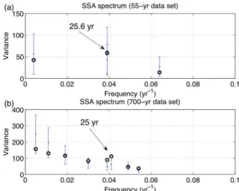
Fig. 7. Monte Carlo SSA spectra of the regime occurrence fre-quency records for the coupled model with a wind-driven oceanic component. The spectra are based on (a) a 55-yr segment of the model simulation; and (b) the entire 700-yr simulation. Error bars represent the 95% confidence interval associated with a red-noise null hypothesis.
mono-polar SST patterns in the North Atlantic with a sub-decadal time scale. Both of these signals are thus different, in terms of their period, from our 25-yr oscillation. Latif et al. (2004) reported mono-polar SST patterns evolving on a time scale of 20–30 yr; however, the centre of action of this oscillation was located, in general, to the northeast of that in Fig. 3. The spatiotemporal signal associated with our Regime A thus represents novel observational features, as well as a novel physical mechanism.
The Hasselman-type conceptual climate models explain a major fraction of SST variance away from the regions of in-tense oceanic currents, viz. oceanic western boundary. This is, of course, also the property of our idealized simulations. Our study is a contribution to the theories of SST variability in the eastward jet extension region, in which passive ocean response explanation is insufficient. In particular, we ar-gue coupled dynamics associated with nonlinear atmospheric sensitivity to ocean-induced eddy-driven SST anomalies is the major component of this variability.
Figures 4 and 5 demonstrate that the bi-decadal climate mode accounts for a major portion of the oceanic heat con-tent variations. The occurrence frequency of the Regimes A and B also exhibits substantially enhanced power in the frequency range associated with the decadal variability. On the other hand, the atmospheric regimes themselves are rel-atively rare events (see Fig. 2b), so that a large part of the atmospheric variability has simply nothing to do with the regime behaviour. Similarly, the SST patterns forced by in-trinsic atmospheric variability not associated with the cou-pled mode under consideration account for a large fraction of SST variance away from the eastward jet extension region.
However, as far as sources of climate predictability and the associated dynamics are concerned, it is useful to identify measures of climatic variability which best describe poten-tially predictable climate modes. For example, the atmo-spheric regimes are but a small fraction of full atmoatmo-spheric variability, but we argue that their occupation frequency is a successful and useful measure of the atmospheric response to ocean-induced SST anomalies.
The coupled adjustment mode mechanism proposed by Kravtsov et al. (2006b, 2007a) is not the only one avail-able for the explanation of mono-polar circulation anomalies arising in eddy-permitting and eddy-resolving ocean mod-els. One viable alternative to this mechanism is the so-called gyre-mode mechanism, which has been documented in a hi-erarchy of increasingly realistic ocean-only models (Jiang et al., 1995; Speich et al., 1995; Simonnet, 2005; Simonnet et al., 2003a, b, 2006; Dijkstra and Ghil, 2006). The time scales of a gyre mode are inter-annual, i.e. somewhat shorter that inter-decadal time scales reported here. However, Simon-net (2005) has shown that under certain conditions the gyre mode can exhibit longer time scale harmonics depending on the number of eastward-jet meanders accommodated by the ocean basin. Another alternative is the turbulent oscillator mechanism proposed recently by Berloff et al. (2007a); the central feature of this mechanism is the “negative viscosity” eddy fluxes maintaining an inter-decadal oscillation. Dis-criminating between potential mechanisms for the observed inter-annual-to-inter-decadal mid-latitude climate variability requires further research.
Regardless of the observed oscillations being ocean-only or coupled phenomena, their atmospheric manifestations re-quire a mechanism for the ocean-induced SST anomalies to induce long-term changes in the atmospheric circulation pat-terns. We have conjectured that this mechanism involves nonlinear sensitivity of the atmospheric weather regimes – a few anomalously persistent atmospheric flow anomalies, whose occurrence frequency depends on the oceanic state. In our observational analysis, these regimes are associated with the bimodal probability density function constructed in the phase space of the leading zonal-flow EOFs. Whether the atmospheric flow is bimodal or not is still a subject of an ongoing debate. Hsu and Zwiers (2001) and Stephenson et al. (2004) argued that the single-regime null hypothesis cannot be rejected due to insufficient amount of data; this argument was, however, rebutted by Deloncle et al. (2007). Berner and Branstator (2007) identified significant deviations from gaussianity in a four-dimensional phase space of an at-mospheric general circulation model and showed that these deviations can be described in terms of two off-centred Gaus-sian distributions. This is consistent with the behaviour of our atmospheric model in the sense that the latter model pro-duces only weakly bimodal or strongly skewed uni-modal probability density functions, but is still bi-stable in each case, i.e., characterized by two distinctive, anomalously per-sistent atmospheric states. This bi-stability in the model is
responsible for the atmospheric sensitivity to ocean-induced SST anomalies, which is an essential part of the simulated coupled cycle.
The idealized models used in our study to interpret obser-vational results are but metaphors of the real climate system. In particular, the ocean–atmosphere interaction in the atmo-spheric QG channel is parameterized using bulk formulas in-volving SST and the atmospheric temperature; the latter is related to the instantaneous depth of the atmospheric layers. In turn, the heat fluxes induce, in the QG framework, the entrainment mass fluxes from one atmospheric layer to the other, thus changing the atmospheric temperature. In reality, air–sea interaction involves a much more complex boundary layer and interior dynamics. Other aspects of atmospheric model that may need additional sensitivity checks include the extreme vertical truncation to two layers, as well as the channel, rather than spherical geometry. The ocean models may be altered in a variety of ways as well, making them progressively more realistic. For example, it is known that neglecting bottom topography can lead to spurious decadal variability in ocean models (Winton, 1997), so modifying flat-bottom geometry of our models is one of the venues for future research. In summary, the modelling aspect of our study is just the first step in the hierarchy of climate models (Ghil and Robertson, 2000), in which one tries to inter-relate aspects of observations, idealized models, and state-of-the-art general circulation models. We plan to continue working further in this direction.
The expressions of geopotential height anomalies asso-ciated with the inter-decadal coupled mode reported here, while strongly zonal, are intensified in the North Atlantic in a pattern not unlike the North Atlantic Oscillation. It can be claimed that our search for this mode was motivated by process climate modelling studies based on models of inter-mediate complexity. The need for process modelling rests in the apparent participation of ocean turbulence in the cou-pled evolution. Current state-of-the-art coucou-pled general cir-culation models do not resolve this turbulence, mostly for computational reasons. This would not represent a problem if accurate parameterizations of eddy dynamics were known. While currently a topic of active research, viable parameter-izations are as yet unavailable.
The connections found here between the decadal variabil-ity of the upper-ocean three-dimensional circulation and non-linear atmospheric regimes are novel and interesting. On the other hand, the drastic differences between the two employed ocean models – a highly resolved turbulent ocean with a somewhat extreme, three-layer, vertical truncation, versus a truly three-dimensional model, but with coarse horizon-tal resolution – rather naturally motivates the question of the sensitivity of low-frequency buoyancy-driven variability to mesoscale turbulence. Inasmuch as ocean eddies are effec-tive at heat transport, it remains a distinct possibility that the adjustment and intrinsic variability of a turbulent buoyancy-driven cells differs qualitatively and quantitatively from that
seen in low Reynolds number models like the one used in this paper. How the apparent connections between atmospheric bi-stability and coupled climate dynamics would be affected in a high Reynolds number model of this type is unknown and worthy of study. Indeed, the broad spectrum of explo-ration remaining to be done on the phenomena reported here identify our results as preliminary, but they do quantitatively advance a new, highly nonlinear paradigm for mid-latitude climate variability that is important to examine. Their prac-tical significance is in ascribing a significant fraction of the observed long-term climate variability to natural causes, thus helping to isolate and better explain human-induced climate changes.
Appendix A
Singular spectrum analysis
To analyze the characteristics of the time series of regime oc-currence in observations, as well as in our coupled models, we have used Singular Spectrum Analysis (SSA) (Broom-head and King, 1986; Fraedrich, 1986; Vautard and Ghil, 1989; Ghil et al., 2002). SSA finds eigenvalues and eigen-vectors of the covariance matrix computed for an augmented vector time series; the latter time series consists of the orig-inal vector and M lagged copies thereof. The window size
M determines the range of periodicities to be detected. The
eigenvectors of the covariance matrix so constructed are called T-EOFs; the associated temporal principal compo-nents (T-PCs) are the time series obtained by projecting the original augmented vector time series onto the T-EOFs. SSA identifies an oscillation in the time series when two consecu-tive eigenvalues of the covariance matrix (ordered by size) are nearly equal, the corresponding T-EOFs are periodic, with the same period and in quadrature, while the associated T-PCs are in quadrature as well. We apply, in addition to the criteria above, a Monte Carlo test (Allen et al., 1996; Allen and Robertson, 1996) to determine the statistical significance of the oscillation detected by SSA.
When the procedure above ascertains the presence of an oscillation, we also compute the so-called SSA reconstruc-tion (Broomhead and King, 1986; Ghil and Vautard, 1991; Ghil et al., 2002) for the oscillation being considered; this reconstruction is based on the corresponding pair of recon-structed components (RCs). The RC pairs are narrow-band filtered versions of the original time series, where the filters are derived data-adaptively from the time series itself, in or-der to maximize the variance captured.
Applying Monte Carlo SSAs to the 55-yr record of the ob-served Regime A and Regime B occurrence frequency yields the spectra in Fig. 6a and b, respectively.
SSA detects the presence of two clear oscillatory pairs, with periods of 25 and 12 yr respectively. While they both fail the Monte Carlo significance test, due to the fairly short time series available, the lagged-correlation analyses
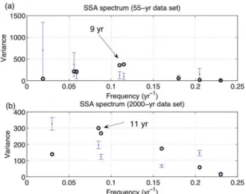
Fig. 8. Same as in Fig. 7, but for the coupled model with a buoyancy-driven oceanic component.
presented in the main text do identify SST patterns with re-gions of statistically significant anomalies at multi-year lags that are consistent with the period detected by SSA.
Similar analyses for the time series of regime occurrence frequency produced by coupled models with wind-driven and buoyancy-driven oceanic components are shown in Figs. 7 and 8, respectively. In either figure, the upper panel is based on a 55-yr segment of the corresponding time series, while the lower panel employs a much longer, multi-centennial model integration.
For the coupled model with the wind-driven oceanic com-ponent (Fig. 7), the dominant oscillation period identified by the SSA employing short and long data sets match quite well: 25.6 yr in the short record, and 25 yr in the long one. More-over, the statistical significance of the oscillatory pairs ac-cording to the Monte Carlo test is considerably larger in the longer data set. In particular, the oscillatory pair based on the short time series fails this test at the 95% level (Fig. 7a), like the one based on the Regime A time series (Fig. 6a), while a longer time series does show statistical significance for the same oscillatory pair at this level.
For the coupled model with the buoyancy-driven oceanic component (Fig. 8), SSA analysis of both the short and long records of regime occurrence frequency does show statisti-cal significance at the 95% level, while the observed spec-trum (Fig. 6b) does not. This has to do with the fact that the 11-yr oscillation in the coupled model is more pronounced than in the data. On the other hand, there is a larger dis-crepancy between the periods in Fig. 8a vs. b, namely 9 yr vs. 11 yr, which indicates some period modulation in the cou-pled model.
To conclude, the SSA analysis identifies oscillatory pairs in the observed and model-generated time series of regime occurrence frequency. The 55 yr of observational record are
not enough to establish statistical significance of these sig-nals at the 95% level. The complementary lagged-regression analysis of SST fields presented in the main text does find sta-tistically significant patterns at multi-year lags that are con-sistent with the periods identified by SSA.
Appendix B
Non-parametric Monte Carlo significance test
We have used the following technique to ascertain statisti-cal significance associated with the quantities derived from the time series of regime occurrence frequency (Vautard et al., 1990). First, we gathered into time segments the con-secutive days belonging to a given regime, including the null regime defined as all data points that do not belong to either of the two regimes identified. These segments were shuffled 1000 times, thus providing 1000 independent realizations of the same length. Each quantity that was estimated using the actual regime time series (for example, regime occurrence frequency, as well as SST fields regressed on this time se-ries at various lags) was also computed using the 1000 shuf-fled sets of category numbers. The 95% confidence level was defined as the 95th percentile of the random values so com-puted, sorted in ascending order.
Acknowledgements. It is a pleasure to thank D. Kondrashov and A. W. Robertson for helpful discussions. We are also indebted to J. Willis, S. L. Marcus, and J. O. Dickey for sharing with us their insights into and interpretation of the upper-ocean heat content observations. J. Willis kindly provided the data used to produce Fig. 4 of the present paper. We are grateful to R. Scott and an anonymous reviewer for their valuable comments, which helped to improve the presentation. This research was supported by NSF grant OCE-02-221066, DOE grants DE-FG-03-01ER63260 and DE-FG02-02ER63413, as well as NASA grant NNG-06-AG66G-1 (MG & SK). PB has also been supported by the Newton Trust research grant, and SK - by the University of Wisconsin-Milwaukee Research Growth Initiative program 2006-2007.
Edited by: R. Grimshaw
Reviewed by: two anonymous referees
References
Allen, R. M. and Smith, L. A.: Monte Carlo SSA: Detecting irreg-ular oscillations in the presence of colored noise, J. Climate, 9, 3373–3404, 1996.
Allen, M. R. and Robertson, A. W.: Distinguishing modulated os-cillations from coloured noise in multivariate data sets, Clim. Dy-nam., 12, 775–784, doi:10.1007/s003820050142, 1996. Broomhead, D. S. and King, G. P.: Extracting qualitative dynamics
from experimental data, Physica D, 20, 217–236, 1986. Berloff, P.: On rectification of randomly forced flows, J. Mar. Res.,
31, 497–527, 2005.
Berloff, P., Hogg, A., and Dewar, W.: The turbulent oscillator: A mechanism of low-frequency variability of the wind-driven ocean gyres, J. Phys. Oceanogr., 37, 1103–1121, 2007a. Berloff, P., Dewar, W. K., Kravtsov, S., McWilliams, J. C., and
Ghil, M.: Ocean eddy dynamics in a coupled ocean–atmosphere model, J. Phys. Oceanogr., 37, 1103–1121, 2007b.
Berner, J. and Branstator, G.: Linear and nonlinear signatures of the planetary wave dynamics of an AGCM: Probability density functions, J. Atmos. Sci., 64, 117–136, doi:10.1175/JAS3822.1, 2007.
Czaja, A. and Marshall, J.: Observations of atmosphere–ocean cou-pling in the North Atlantic, Q. J. Roy. Meteor. Soc., 127, 1893– 1916, 2001.
Deloncle, A., Berk, R., D’Andrea, F., and Ghil, M.: Weather regime prediction using statistical learning, J. Atmos. Sci., 64, 1619– 1635, 2007.
Delworth, T. and Mann, M.: Observed and simulated multidecadal variability in the Northern Hemisphere, Clim. Dynam., 16, 16 661–16 676, doi:10.1007/s003820000075, 2000.
Deser, C.: On the teleconnectivity of the “Arctic Oscillation,” Geophys. Res. Lett., 27, 779–782, doi:10.1029/1999GL010945, 2000.
Deser, C. and Blackmon, M. L.: Surface climate varia-tions over the North Atlantic Ocean during winter: 1900– 1989, J. Climate, 6, 1743–1753, doi: 10.1175/1520-0442(1993)006<1743:SCVOTN>2.0.CO;2, 1993.
Dijkstra, H. A. and Ghil, M.: Low-frequency variability of the large-scale ocean circulation: A dynamical systems approach, Rev. Geophys., 43, RG3002, doi:10.1029/2002RG000122, 2005. Dong, B. and Sutton, R.: Mechanism of interdecadal thermohaline circulation variability in a coupled ocean–atmosphere model, J. Climate, 18, 1117–1135, doi:10.1175/JCLI3442.1, 2005. Fraedrich, K.: An observational study of intraseasonal poleward
propagation of zonal mean flow anomalies, J. Atmos. Sci., 43, 419–432, 1986.
Ghil, M. and Robertson, A. W.: Solving problems with GCMs: General circulation models and their role in the climate mod-eling hierarchy, General Circulation Model Development: Past, Present and Future, edited by: Randall, D., Academic Press, San Diego, pp. 285–325, 2000.
Ghil, M. and Vautard, R.: Interdecadal oscillations and the warming trend in global temperature time series, Nature, 350, 324–327, doi:10.1038/350324a0, 1991.
Ghil M., Allen, M. R., Dettinger, M. D., Ide, K., Kondrashov, D., Mann, M. E., Robertson, A. W., Saunders, A., Tian, Y., Varadi, F., and Yiou, P.: Advanced spectral methods for climatic time series, Rev. Geophys., 40(1), 1003 doi:10.1029/2000RG000092, 2002.
Gr¨otzner, A., Latif, M., and Barnett, T. P.: A decadal climate cycle in the North Atlantic Ocean as simulated by the ECHO coupled GCM, J. Climate, 11, 831–847, doi:10.1175/1520-0442(1998)011<0831:ADCCIT>2.0.CO;2, 1998.
Hasselmann, K.: Stochastic climate models, Part I: Theory, Tellus, 28, 289–305, 1976.
Hsu, C. J. and Zwiers, F.: Climate change in recurrent regimes and modes of Northern Hemisphere atmospheric variability, J. Geo-phys. Res., 106(D17), 20,145–20,160, 2001.
Hurrell, J. E.: Decadal trends in the North Atlantic Oscillation: Re-gional temperatures and precipitation, Science, 269, 676–679,
doi:10.1126/science.269.5224.676, 1995.
Jiang, S., Jin, F.-F., and Ghil, M.: Multiple equilibria, periodic and aperiodic solutions in a wind-driven, double-gyre, shallow-water model, J. Phys. Oceanogr., 25, 764–786, 1995.
Kalnay, E., Kanamitsu, M., Kistler, R., et al.: The NCEP/NCAR 40-year reanalysis project. B. Am. Meteorol. Soc., 77, 437–471, doi:10.1175/1520-0477(1996)077<0437:TNYRP>2.0.CO;2, 1996.
Koo, S., Robertson, A. W., and Ghil, M.: Multiple regimes and low-frequency oscillations in the Southern Hemi-sphere’s zonal-mean flow, J. Geophys. Res., 107(D21), 4596, doi:10.1029/2001JD001353, 2003.
Kravtsov, S. and Ghil, M.: Interdecadal variability in a hybrid coupled ocean-atmosphere-sea-ice model, J. Phys. Oceanogr., 34, 1756–1775, doi:10.1175/1520-0485(2004)034<1756:IVIAHC>2.0.CO;2, 2004.
Kravtsov, S., Robertson, A. W., and Ghil, M.: Bimodal behavior in the zonal mean flow of a baroclinic beta-channel model, J. Atmos. Sci., 62, 1746–1769, doi:10.1175/JAS3443.1, 2005. Kravtsov, S., Robertson, A. W., and Ghil, M.: Multiple regimes and
low-frequency oscillations in the Northern Hemisphere’s zonal-mean flow, J. Atmos. Sci., 63, 840–860, doi:10.1175/JAS3672.1, 2006a.
Kravtsov, S., Berloff, P., Dewar, W. K., Ghil, M., and McWilliams, J. C.: Dynamical origin of low-frequency variability in a highly-nonlinear mid-latitude coupled model, J. Climate, 19, 6391– 6408, doi:10.1175/JCLI3976.1, 2006b.
Kravtsov, S., Dewar, W. K., Berloff, P., McWilliams, J. C., and Ghil, M.: A highly nonlinear coupled mode of decadal variability in a mid-latitude ocean–atmosphere model, Dyn. Atmos. Oceans, 43, 123–150, doi:10.1016/j.dynatmoce.2006.08.001, 2007a. Kravtsov, S., Dewar, W. K., Ghil, M., McWilliams, J.
C., and Berloff, P.: A mechanistic model of mid-latitude decadal climate variability, Physica D, in press, doi:10.1016/j.physd.2007.09.025, 2007b.
Kushnir, Y.: Interdecadal variations in North Atlantic sea surface temperature and associated atmospheric con-ditions, J. Climate, 7, 141–157, doi:10.1175/1520-0442(1994)007<0141:IVINAS>2.0.CO;2, 1994.
Latif, M. and Barnett, T. P.: Decadal climate variability over the North Pacific and North America: Dynamics and predictability, J. Climate, 9, 2407–2423, doi:10.1175/1520-0442(1996)009<2407:DCVOTN>2.0.CO;2, 1996.
Latif, M., Roeckner, E., Botzetet, M., et al.: Reconstruct-ing, monitorReconstruct-ing, and predicting multidecadal-scale changes in the North Atlantic thermohaline circulation with sea surface temperature, J. Climate, 17, 1605–1614, doi:10.1175/1520-0442(2004)017<1605:RMAPMC>2.0.CO;2, 2004.
Levitus, S.: Interpentadal variability of temperature and salin-ity at intermediate depths of the North Atlantic Ocean: 1970– 1974 versus 1955–1959, J. Geophys. Res., 94, 6091–6131, doi:10.1029/89JC01436, 1989.
Levitus, S. J., Antonov, I., and Boyer, T. P.: Warming of the world ocean, 1955 – 2003, Geophys. Res. Lett., 32, L02604, doi:10.1029/2004GL021592, 2005.
Lyman, J. M., Willis, J. K., and Johnson, G. C.: Recent cool-ing of the upper ocean, Geophys. Res. Lett., 33, L18604, doi:10.1029/2006GL027033, 2006.
Mantua, N. J., Hare, S. R., Zhang, Y., Wallace, J. M., and Francis,
R. C.: A Pacific interdecadal climate oscillation with impacts on salmon production, B. Am. Meteorol. Soc., 78, 1069–1079, doi:10.1175/1520-0477(1997)078<1069:APICOW>2.0.CO;2, 1997.
Marshall, J., Johnson, H., and Goodman, J.: A study of the interac-tion of the North Atlantic Oscillainterac-tion with ocean circulainterac-tion, J. Climate, 14, 1399–1421, 2000.
Marshall, J., Kushnir, Y., Battisti, D., Chang, P., Czaja, A., Dick-son, R., Hurrell, J., McCartney, M., Saravanan, R., and Visbeck, M.: North Atlantic climate variability: Phenomena, impacts and mechanisms, Int. J. Climatol., 21, 1863–1898, 2001.
Mehta, V. M., Suarez, M. J., Manganello, J. V., and Delworth T. L.: Oceanic influence on the North Atlantic oscillation and associ-ated Northern Hemisphere climate variations: 1959 - 1993, Geo-phys. Res. Lett., 27(1), 121–124, doi:10.1029/1999GL002381, 2000.
Moron, V., Vautard, R., and Ghil, M.: Trends, interdecadal and in-terannual oscillations in global sea-surface temperatures, Clim. Dynam., 14, 545–569, doi:10.1007/s003820050241, 1998. Pierce, D. W., Barnett, T. P., Schneider, N., Saravanan, R.,
Dom-menget, D., and Latif, M.: The role of ocean dynamics in pro-ducing decadal climate variability in the North Pacific, Clim. Dy-nam., 18, 51–70, doi:10.1007/s003820100158, 2001.
Power, S. and Colman, R.: Multi-year predictability in a cou-pled general circulation model, Clim. Dynam., 26, 247–272, doi:10.1007/s00382-005-0055-y, 2006.
Robertson, A. W.: Influence of ocean–atmosphere interac-tion on the Arctic Oscillainterac-tion in two general circula-tion models, J. Climate, 14, 3240–3254, doi:10.1175/1520-0442(2001)014<3240:IOOAIO>2.0.CO;2, 2001.
Rodwell, M. J., Rodwell, D. P., and Folland, C. K.: Oceanic forc-ing of the wintertime North Atlantic Oscillation and European climate, Nature, 398, 320–323, doi:10.1038/18648, 1999. Saravanan, R.: Atmospheric low-frequency variability and its
relationship to midlatitude SST variability: Studies using NCAR Climate System Model, J. Climate, 11, 1386–1404, doi:10.1175/1520-0442(1998)011<1386:ALFVAI>2.0.CO;2, 1998.
Schlesinger, M. E. and Ramankutty, N.: An oscillation in the global climate system of period 65–70 years, Nature, 367, 723–726, doi:10.1038/367723a0, 1994.
Simonnet, E.: Quantization of the low-frequency variability of the double-gyre circulation, J. Phys. Oceanogr., 35, 2268–2290, 2005.
Simonnet, E., Ghil, M., Ide, K., Temam, R., and Wang, S.: Low-frequency variability in shallow-water models of the wind-driven ocean circulation. Part I: Steady-state solutions, J. Phys. Oceanogr., 33, 712–728, 2003a.
Simonnet, E., Ghil, M., Ide, K., Temam, R., and Wang, S.: Low-frequency variability in shallow-water models of the wind-driven ocean circulation. Part II: Time-dependent solutions, J. Phys. Oceanogr., 33, 729–752, 2003b.
Simonnet, E., Ghil, M., and Dijkstra, H. A.: Homoclinic bifurca-tions in the quasi-geostrophic double-gyre circulation, J. Mar. Res., 63, 931–956, 2006.
Speich, S., Dijkstra, H., and Ghil, M.: Successive bifurcations in a shallow-water model, applied to the wind-driven ocean circula-tion, Nonlin. Proc. Geophys., 2, 241–268, 1995.
of multiple climate regimes, Q. J. Roy. Meteor. Soc., 130, 583– 605, 2004.
Sutton, R. T. and Allen, M. R.: Decadal predictability in North At-lantic sea surface temperature and climate, Nature, 388, 563– 567, 1997.
Vautard, R. and Ghil, M.: Singular spectrum analysis in nonlinear dynamics, with applications to paleoclimatic time series, Physica D, 35, 395–424, 1989.
Vautard, R., Mo, K.-C., and Ghil, M.: Statistical signif-icance test for transition matrices of atmospheric Markov chains, J. Atmos. Sci., 47, 1926–1931, doi:10.1175/1520-0469(1990)047<1926:SSTFTM>2.0.CO;2, 1990.
Winton, M.: The damping effect of bottom topography on inter-nal decadal-scale oscillations of the thermohaline circulation, J. Phys. Oceanogr., 27, 203–208, 1997.