HAL Id: halshs-01318093
https://halshs.archives-ouvertes.fr/halshs-01318093
Submitted on 19 May 2016
HAL is a multi-disciplinary open access
archive for the deposit and dissemination of sci-entific research documents, whether they are pub-lished or not. The documents may come from teaching and research institutions in France or
L’archive ouverte pluridisciplinaire HAL, est destinée au dépôt et à la diffusion de documents scientifiques de niveau recherche, publiés ou non, émanant des établissements d’enseignement et de recherche français ou étrangers, des laboratoires
Risk Measures At Risk- Are we missing the point?
Discussions around sub-additivity and distortion
Dominique Guegan, Bertrand K. Hassani
To cite this version:
Dominique Guegan, Bertrand K. Hassani. Risk Measures At Risk- Are we missing the point? Discus-sions around sub-additivity and distortion. 2016. �halshs-01318093�
Documents de Travail du
Centre d’Economie de la Sorbonne
Risk Measures At Risk- Are we missing the point?
Discussions around sub-additivity and distortion
Dominique G
UEGAN,Bertrand K. H
ASSANIRisk Measures At Risk- Are we missing the point?
Discussions around sub-additivity and distortion
April 29, 2016
Dominique GUEGAN1, Bertrand K. HASSANI2.
Abstract
This paper3 discusses the regulatory requirements (Basel Committee, ECB-SSM and
EBA) to measure the major risks of financial institutions, for instance Market, Credit and Operational, regarding the choice of the risk measures, the choice of the distributions used to model them and the level of confidence. We highlight and illustrate the paradoxes and issues observed when implementing one approach over another, the inconsistencies between the methodologies suggested and the goals required to achieve them. We focus on the notion of sub-additivity and alternative risk measures, providing the supervisor with some recom-mendations and risk managers with some tools to assess and manage the risks in a financial institution4.
1
Université Paris 1 Panthéon-Sorbonne, CES UMR 8174, 106 boulevard de l’Hopital 75647 Paris Cedex 13, France, phone: +33144078298, e-mail: [email protected]
2Grupo Santander and Université Paris 1 Panthéon-Sorbonne CES UMR 8174, 106 boulevard de l’Hopital 75647 Paris Cedex 13, France, phone: +44 (0)2070860973, e-mail: [email protected]. Disclaimer: The opinions, ideas and approaches expressed or presented are those of the authors and do not necessarily reflect Santander’s position. As a result, Santander cannot be held responsible for them.
3This work was achieved through the Laboratory of Excellence on Financial Regulation (Labex ReFi) supported by PRES heSam under the reference ANR-10-LABEX-0095
4
This paper has been written over a very specific period of time as most regulatory papers written in the past 20 years are currently being questioned by both practitioners and regulators themselves. Some disarray has been observed among risk managers as most models required by the regulations have not been consistent with their own objective of risk management. The enlightenment brought by this paper is based on an academic analysis of the issues engendered by some pieces of regulation and its purpose is not to create any sort of controversy.
Key words: Risk measures - Sub-additivity - Level of confidence - Distributions - Financial regulation - Distortion - Spectral measure
1
Introduction
The ECB-SSM5, the EBA 6 and the Basel Committee are currently reviewing the methodolog-ical framework of risk modelling. In this paper, we analyse some of the issues observed when measuring the prescribed risks that would be worth addressing in future regulatory documents.
1.1 Problematic
During the current crisis, the failure of models and the lack of capture of extreme exposures have led regulators to change the way risks are measured, either by requiring financial institu-tions to use particular families of distribuinstitu-tions (Gaussian (BCBS (2005)), sub-exponential (EBA (2014b))), or by changing the way dependencies are captured (EBA (2014b)) or by suggesting a change from the Value-at-Risk (VaR)7 to sub-additive risk measures like the Expected Shortfall (ES)8 (BCBS (2013)). Indeed, risk modelling had played a major role during the crisis which began in 2008 either as a catalyst or trigger. The latest changes proposed by the authorities have been motivated by the will to come closer to the reality of financial markets.
In a recent paper we have discussed the importance of the choice of the distributions in mea-suring the risks (Guégan and Hassani (2016)). In this paper we focus on the role of the notion of sub-additivity which interested many researchers around 2000 (Artzner et al. (1999), Jorion
5
European Central Bank - Single Supervisor Mechanism 6
European Banking Authority 7
Given a confidence level p ∈ [0, 1], the VaR associated to a random variable X is given by the smallest number
x such that the probability that X exceeds x is not larger than (1 − p)
V aRp= inf(x ∈ R : P (X > x) ≤ (1 − p)). (1.1)
8For a given p in [0, 1], η the V aR
p, and X a random variable which represents losses during a pre-specified
period (such as a day, a week, or some other chosen time period) then,
(2006)) and brought about a change in the requirements from regulators since 2010 (BCBS (2011a), BCBS (2011b), BCBS (2013), EBA (2014a)). The question is to understand if this problematic is really interesting from a practical point of view, and to help address the objective set by the regulation. We will also discuss in more detail the interest of other risk measures like the spectral risk measure and a new way to take into account extreme events using distortion risk measures.
Thus, the purpose of this paper is to discuss some methodological aspects of the regulatory framework related to risk modelling and its evolution since 1995, focusing on supervisors’ strong incentive to use: (i) specific distributions to characterise the risks, (ii) specific risk measures, (iii) specific associated confidence level, and to apply these strategies independently from each other. We argue that the approaches proposed by the regulator engender a bias (positive or negative) in the assessment of the risks, and consequently a distortion in both the corresponding capital requirements and the management decision taken since the problem of the measurement is not dealt with in its entirety.
Some of the following points are addressed in this paper: (i) Is the choice of a particular risk measure ensuring conservativeness? (ii) When moving from a V aRp to sub-additive risk mea-sures such as the ESp, for which distributions is the sub-additivity9 property fulfilled given that
we consider several risk factors? (iii) Given that each risk type is modelled based on different distributions and using different p-s, how can the sub-additivity criterion be fulfilled? Is that really important in practice? These different points are linked to the choice of a particular dis-tribution and to the choice of the confidence level p.
The regulatory documents state with respect to market risk since 1995 (BCBS for instance)
-9A coherent risk measure is a function ρ : L∞ → R:
• Monotonicity:If X1, X2∈ L and X1≤ X2 then ρ(X1) ≤ ρ(X2) • Sub-additivity: If X1, X2∈ L then ρ(X1+ X2) ≤ ρ(X1) + ρ(X2) • Positive homogeneity: If λ ≥ 0 and X ∈ L then ρ(λX) = λρ(X) • Translation invariance: ∀k ∈ R, ρ(X + k) = ρ(X) − k
that "the VaR risk measure is inadequate for measuring the risks because it does not take into account the extreme events" and also "one of the problems of recognising banks’ value-at-risk measures as an appropriate capital charge is that the assessments are based on historical data and that, even under a 99% confidence interval, extreme market conditions are excluded". To confirm this fact, in the Consultative Document concerning the Fundamental review of the trad-ing book (BCBS (2013)), the Basel Committee proposes "to move from Value-at-Risk (VaR) to Expected Shortfall (ES) as a number of weaknesses have been identified using VaR for determin-ing regulatory capital requirements, includdetermin-ing its inability to capture tail risk". The Committee has agreed "to use a 97.5th ES for the internal models-based approach and to use it to calibrate capital requirements under the revised market risk standardised approach".
In these documents the regulator says that the choice of the VaR as a risk measure does not take into account extreme values. This statement is not correct as the choice of the VaR is not the issue; it is the choice of the underlying distribution with which the associated quantile is evaluated that determines if the extreme events are captured or not. This question actually implies a second question about what an extreme event is and answering this question would suppose a complete information set. Then in 2013, it seems that the regulator thought that the use of the ES instead of the VaR is more effective at capturing the most relevant information to measure the risks. This is not necessarily true as once again, it depends on the choice of the distributions used for the computation of this ES. Nevertheless, we know that this last measure is more interesting than the VaR when considering the same distribution because it provides better information concerning the amplitude of the risk, but if the fitted distribution is inap-propriate the problem of capturing extreme events remains the same. Besides, the choice of the level of confidence, for instance 97.5 is also arbitrary (this point will be illustrated in the next section). Indeed, why did the regulator move from 99% (in 1995) to 97.5 % (in 2013)? - Why did they not suggest 95% or another value p?
Another point is considered by the regulators for operational risk modelling, see EBA (2014b)10. In these documents they consider that a "risk measure means a single statistic extracted from the aggregated loss distribution at the desired confidence level, such as Value-at-Risk (VaR), or
10
shortfall measures (e.g. Expected Shortfall, Median Shortfall)". This definition is particularly limiting and dangerous. How can the risk measures computed for different factors with different levels be aggregated? If we use the ES measure, it loses its sub-additivity property in that latter case. Thus, other approaches could be more robust and realistic, for instance the use of spectral measure.
It appears that some documents are too prescriptive, preventing banks from going beyond the proposals and focusing more on the capital calculations than on the risk management itself. Regarding the calculation of the capital requirement from the knowledge of the risk factors, the main points concern the choice of the distribution, the choice of the risk measure and the choice of p: these choices are not studied in a uniform way and the approach proposed by the regulators does not constitute a robust approach for measuring the risk of a bank.
In Section Two, we investigate the notion of sub-additivity for a risk measure showing that this property also depends on the choice of the distribution and not only on the choice of the risk measure. We illustrate the point that the restriction imposed by regulators prevents a reliable approach to measure the risk. We illustrate our statements with examples. In Section Three we show that it is the choice of the distributions which is definitively the key point in risk modelling. Then in Section Four, we propose a new way to measure the risk, working in two directions; using the spectral measure and/or using a measure based on the distortion of the distribution in order to have multi-modal distributions to model the risk factors. Section Five concludes.
2
Sub-additivity property: a real added-value for risk
manage-ment?
The concept of sub-additivity which has been largely studied in the 2000’s appears interesting if we consider that the measure of the risk of a portfolio11 is obtained when we calculate the risks of each factor of this portfolio. This is a very restrictive approach for measuring these exposures. An appropriate solution would be to use a multivariate quantile approach based on copula or vines (Guégan and Maugis (2010a), Guégan and Hassani (2013), etc). Nevertheless,
if we maintain this method of calculating the risks, the idea of the sub additive risk measure is that the measure of the sum has to be smaller than the sum of the risk, and following the works of Artzner et al. (1999), it seems that this property is only verified by the ES risk mea-sure. In fact, this property is also verified by the VaR measure: it depends on the distribution used (Degen and Embrechts (2008)). Indeed, VaR is known to be sub-additive (i) for stable distribution, (ii) for all log-concave distribution, (iii) for the infinite variance stable distributions with finite mean, (iv) and for distribution with Generalised Pareto Distribution type tails when the variance is finite. The non-sub-additivity of VaR can occur (i) when assets in portfolios have greatly skewed loss distributions; (ii) when the loss distributions of assets are smooth and symmetric, (iii) when the dependency between assets is highly asymmetric, and (iv) when un-derlying risk factors are independent but very heavy-tailed. To illustrate our purpose, we have selected a data set provided by a Tier European bank representing "Execution, Delivery and Process Management" risks from 2009 to 2014. "Execution, Delivery and Process Management" risk is a sub-category of operational risk12. This data set is characterised by a distribution right skewed (positive skewness) and leptokurtic.
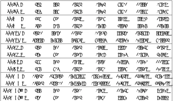
In order to follow the regulatory guidelines, we choose to fit on this data set some of the dis-tributions prescribed and also others which seem more appropriate regarding the properties of the data set. We retain seven distributions. They are estimated (i) on the whole sample: the empirical distribution, the lognormal distribution (asymmetric and medium tailed), the Weibull distribution (asymmetric and thin tailed), a Generalised Hyperbolic (GH) distribution (symmet-ric or asymmet(symmet-ric, fat tailed on an infinite support), an Alpha-Stable distribution (symmet(symmet-ric, fat tailed on an infinite support), a Generalised Extreme value (GEV) distribution (asymmetric and fat tail), (ii) on an adequate subset: the Generalised Pareto (GPD) distribution (asymmet-ric, fat tailed) calibrated on a set built over a threshold, a Generalised Extreme Value (GEVbm) distribution (asymmetric and fat tailed ) fitted using maxima coming from the original set. The whole data set contains 98082 data points, the sub-sample used to fit the GPD contains 2943 data points and the sub-sample used to fit the GEV using the block maxima approach contains 3924 data points. The objective of these choices is to evaluate the impact of the selected
dis-12In our demonstration, the data set which has been sanitised here is not of particular importance since the same data set has been used for each and every distribution tested.
tributions on the risk representation, i.e. how the initial empirical exposures are captured and transformed by the model. It is interesting to note that using empirical distributions instead of fitted analytical distributions could be of interest as the former one captures multi-modality by construction. Unfortunately, this solution was initially rejected by regulators as this non-parametric approach is not considered able to capture tails properly which, as shown in the table, might be a false statement. However, recently the American supervisor seems to be re-introducing empirical strategies in practice for CCAR13 purposes.
Table 1 exhibits parameter estimates for each distribution selected14. The parameters are esti-mated by maximum likelihood, except for the GPD which implied a POT (Guégan et al. (2011)) approach and the GEV fitted on the maxima of the data set (maxima obtained using a block maxima method (Gnedenko (1943))). The quality of the adjustment is measured using both the Kolmogorov-Smirnov and the Anderson-Darling tests. The results presented in Table 1 show that none of the distributions is adequate. This is usually the case when fitting uni-modal dis-tributions to a multi-modal data set. Indeed, multi-modality of the disdis-tributions is a frequent issue when modelling operational risks as the risk categories combine multiple kinds of incidents; for instance a category combining external frauds will contain the fraud card on the body, com-mercial paper fraud in the middle, cyber attack and Ponzi scheme in the tail, but we have also observed a similar pattern using market data. It could be more appropriate to consider empirical distributions than fitted analytical distributions as it may help to capture multi-modality. We will come back to this last point in Section 4.
In the introduction we indicated that the regulator recommends the use of the ES instead of the VaR because the former is sub-additive, property unverified by the VaR. In the following section, we question these assertions showing that, even if it is true that the ES is sub-additive, (i) the VaR also has this property for a lot of distributions as we have mentioned before; (ii) the sub-additivity property can be verified for some values of p, and not verified for others; (iii) the sub additivity of the VaR is very often verified for fat-tailed distributions; (iv) the sub-additivity is not verified anymore for the ES when we aggregate them. We illustrate these different facts
13Comprehensive Capital Analysis and Review
14In order not to overload the table the standard deviation of the parameters are not exhibited but are available upon request.
making some simulations computing VaRp(X + Y ) and VaRp(X) + VaRp(Y ) for X and Y two
risk factors. We proceed in the following way:
• As VaRp(X) is a quantile, p ∈ [0, 1], the entire spectrum of the VaR has been built, considering the inverse of the cumulative distribution function. Summing VaRp(X) and
VaRp(Y ) for each value of p provides us with VaRp(X) + VaRp(Y ).
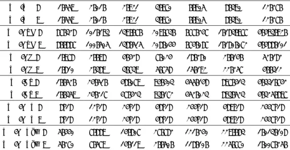
• To obtain VaRp(X +Y ), another approach is adopted. In a first step we randomly generate X and Y using specific distributions. Then X and Y are aggregated. The resulting cumula-tive distribution function is built and its inverse provides the spectrum of VaRp(X + Y )15. In Table 2 we provide the values obtained for both the VaR and the ES for fully correlated random variables. It is interesting to note that the risk measures obtained on fully correlated random variables and the sum of the risk measures obtained univariately are really similar. This means that as soon as we sum the VaR obtained on two variables we mechanically assume an upper tailed correlation for the random variables. Therefore, as well as being conservative, the sum of univariate VaRs taken at the same level prevents the capture of any diversification ben-efit. Fully correlated random variables do not embed any diversification benefit by definition. Consequently, the analysis regarding the sub-additivity of the risk measures has to be performed in another way.
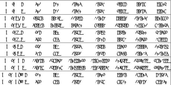
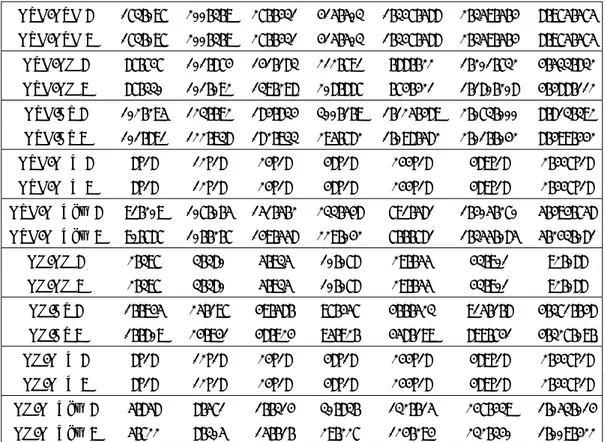
Then we work with the data sets we have previously introduced. We randomly generated val-ues from the distribution fitted before and combined them two by two. By carrying out this process we generated some random correlations and incidentally some diversification. Then, we compared the risk measures obtained from the combination of random variables and the sum of the risk measures computed on the random variables taken independently. From Table 3, for fixed p, we observe that the VaR is never sub-additive if the lognormal distribution is associated with a GPD; while if the lognormal distribution is associated with any of the others, the VaR is usually sub-additive in the tails but not at the end of the body part. Note that if the log-normal is associated with an identical loglog-normal, the differences we have observed are only due to numerical errors related to sampling. We expect the two values to be absolutely identical. However, it is interesting to note that the random generation of numbers can be at the origin of
15
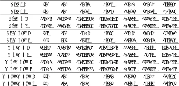
non sub-additive results. An identical analysis can be done on other combinations. From Table 5 it appears that when the GPD has a positive location parameter, this prevents any combina-tion from being sub-additive, because by construccombina-tion the 0th percentile of the GPD is equal to the location parameter which should, according to Pickand’s theorem (Pickands (1975)), be sufficiently high. At the 95th percentile, the VaR is always sub-additive whenever a lognormal distribution is involved, except if it is combined with a GPD. For the other distributions, it is not always true. For example, the VaR obtained after combining a Weibull and a GEV fitted on the whole sample is not sub-additive. Table 6 shows that the use of an Alpha-Stable combined with any other distribution, except for the GPD, provides sub-additive risk measures at the 99% level. Other examples are provided in Table 6 with the Weibull distribution.
Building the ES always leads to sub-additive values (see Tables 7 - 10), contrary to the VaR for which this property is not always verified and depends on the underlying distribution as discussed previously: the results for the ES can be compared to those obtained with the VaR looking at Tables 3 and 7, Tables 4 and 8, then Tables 5 and 9 and finally Tables 6 and 10. It is interesting to note that if we combine two ES measures taken at two different levels of con-fidence p, the ES may not be sub-additive anymore. This is a point that the regulators do not discuss when they imply that the risk measures have to be aggregated. This issue is particularly important for risk managers, since the level of confidence prescribed in the regulation guidelines is different from one risk factor to another and appears totally arbitrary.
In parallel, Figures 5 to 9 allow a more discriminating analysis of the behaviour of the component
V aRp(X +Y ) versus V aRp(X)+V aRp(Y ). In Figure 5, we show that the sub-additivity property
is only verified for high percentiles when we combine a Weibull and a GH distribution, i.e. for
p > 90%. In addition, the gap tends to widen as the percentiles increase. Figure 6 exhibits
a non sub-additive VaR from the 95th percentile, when we use the combination of an Alpha-Stable distribution and a GEV fitted with the block maxima method, but the differences are not as great as in Figure 5. Figure 7 shows that combining two identical distributions does not always produce sub-additive risk measures though it should always be the case: this can be due to numerical errors caused by the random generation of data points and the discretisation of the distribution. In Figures 8 and 9 we observe that the VaRs obtained from the combination
of an Alpha-Stable distribution and a GH distribution or an Alpha-stable distribution and a GEV distribution calibrated on maxima are never sub-additive below 70%. For comparison purposes, Figures 10 and 11 illustrate the fact that the combination of two elliptical distributions (respectively the Gaussian and the Student-t distributions) always leads to sub-additive VaRs.
3
Role of the distributions in the computation of VaR and ES
measures
In this section we illustrate the influence of the distributions on the risk measure evaluations. Table 11 provides the values obtained for the VaRp and the ESp computed from the eight
distri-butions fitted on the data set or some sub-samples. We also illustrate the fact that an a priori on the choice of a distribution provides arbitrary results which can be disconnected from reality.
From Table 11 we note that the values provided by VaRp can be bigger than the values derived
for an ESp and conversely. We observe that the results obtained from the GPD and the alpha-stable distributions are of the same order. Second, the differences between the GPD and the GEV fitted on the block maxima are huge, illustrating the fact that, despite being two extreme value distributions, the information captured is quite different. The ES calculations are also linked to the distribution used to model the underlying risks. Looking at Table 11, at 95%, we observe that the ES goes from 1979 for the Weibull to 224 872 for the GPD. Therefore, depending on the distribution used to model the same risk, at the same p level, the ES obtained is completely different. The corollary of that issue is that the ES obtained for a given distribu-tion at a lower percentile will be higher than the ES computed with another distribudistribu-tion at a higher percentile. For example, Table 11 shows that the 90% ES obtained from an Alpha-Stable distribution is much higher than the 99.9% ES computed on a lognormal distribution.
Thus one question arises. What should the regulator ask to use: the VaR or the Expected Short-fall? To answer this question, we can consider several points: (i) Conservativeness: Regarding that point, the choice of the risk measure is only relevant for a given distribution, i.e. for any given distribution the VaRp will always be inferior to the ESp (assuming only positive values)
a given level p, the VaRp obtained from a distribution is superior to the ESp for another
distri-bution. For example, Table 11 shows that the 99.9% VaR obtained using the GH distribution is superior to the ES obtained for the Weibull or the lognormal distributions at the same level p; (ii) Distribution and p impacts: Table 11 shows that potentially a 90% level ES obtained from a given distribution is larger than a 99.9% VaR obtained with another distribution, e.g. the ES obtained from a GH distribution at 90% is higher than the VaR obtained from a lognormal dis-tribution at 97.5%. Thus is it always pertinent to use a high value for p? (iii) Parameterisation and estimation: the impact of the calibration of the estimates of the parameters is not negligible (Guégan et al. (2011)), for instance when we fit a GPD. Indeed, in that latter case, due to the instability of the estimates of the threshold, the practitioners can largely overfit the risks.
4
Alternative approaches: Spectral measure and Distortion
4.1 Spectral Risk Measure vs Spectrum
In this subsection, we briefly introduce the concept of spectral risk measure as the work pre-sented in this paper can easily be extended to this particular tool. Besides, in order to avoid any mis-understanding, we point out the difference between a spectral risk measure and the spectrum of a risk measure as used in this paper.
A spectral risk measure is obtained considering a weighted average of outcomes. Contrary to the approach discussed above, a spectral risk measure is always a coherent risk measure. Spectral measures found their usefulness in the fact that they can be related to risk aversion through the weights chosen for the possible risk exposures.
Acerbi (2002) introduces the formal notion of spectral risk measure: a spectral risk measure
ρ : L → R is defined by
ρ(X) = −
Z 1 0
φ(p)F−1(x)(p)dp (4.1)
where φ is positive or null, non-increasing, right-continuous, integrable function defined on [0, 1] such thatR1
0 φ(p)dp = 1 and F (x) is the cumulative distribution function for x. Any spectral risk
measure satisfies the following condition making them useful in practice (Adam et al. (2007)): • Positive Homogeneity: for a risk X and positive value ψ > 0, ρ(ψX) = ψρ(X);
• Translation-Invariance: for a risk X and α ∈ R, ρ(X + a) = ρ(X) − a;
• Monotonicity: for any combination of risks X and Y such that X ≥ Y , ρ(X) ≥ ρ(Y );
• Sub-additivity: for any combination of risks, ρ(X + Y ) ≤ ρ(X) + ρ(Y );
• Law-Invariance: for any combination of risks X and Y with respective cumulative distri-bution functions F (x) and F (y), if F (x) = F (y) then ρ(X) = ρ(Y );
• Comonotonic Additivity: for every comonotonic random variables (for instance these ran-dom variables are representing risks) X and Y , ρ(X + Y ) = ρ(X) + ρ(Y ).
Note that the Expected Shortfall discussed in this paper is a spectral risk measure for which
φ(p) = 1, ∀p. However, the VaR is not a spectral risk measure but as discussed below may
have a spectral representation. We refer here to the spectrum of the risk measure, i.e. the value obtained, considering various levels of pi, and justify the use of the spectrum in practice.
Indeed, while the use of several levels pi, i = 1, · · · , k allows a spectral representation of the
risk measures (VaR or ES) and could be interesting for risk management, the approach pro-posed by regulators which combines distribution and confidence level is questionable. Indeed, the 70% ES of some combinations may lead to a much higher value than the 99.9th (Table 8, WE-GPD vs WE-GH); on the contrary we provide in Tables 12, 13 and 14, the differences
V aR(X) + V aR(Y ) − V aR(X + Y ) for several distributions. In Table 12 we use Weibull and
a lognormal distributions, in Table 13 Weibull and α-stable distributions and in Table 14 two GEV distributions. We do this exercise for 90% < p < 99.9% in Tables 12 and 13, and for 1% < p < 99.9% with a step of 1% in Table 14. In that last table when the values are positive, the VaR is sub-additive, when the values are negative it is not sub-additive. The turning points are highlighted in bold. This provides an interesting picture of the property of these distribu-tions. This spectral representation of the VaR given in these tables provides good information in terms of risk management; indeed, it shows that relying directly on risk measures to evaluate a capital requirement may not be representative of the risk profile of the target entity. In fact, it can even be misleading, as from one pi to another because the risk measures may have
dra-matically different orders. The spectrum of the VaR approach shows a risk measure obtained at a particular level cannot be representative of the whole risk profile, and assuming the contrary
could lead to dreadful failure and mismanagement. Thus we can encourage the risk managers to compute the spectrum to have a better understanding of these risks.
4.2 Distorted distributions
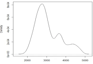
In terms of risks, the first point to consider, as we have seen previously, is to fit a "correct" distribution on the data. Indeed, looking at Figure 1, we observe that the "natural" distribution fitted on the underlying market data16 set is multi-modal. In practice, we often observe this kind of pattern for financial or economic data sets. We observe from this graph that we can sep-arate large losses from the other ones and then obtain a better understanding of the probability of these outcomes. In this section we propose an alternative to paragraph 3 for the fit of the distributions characterising the risk factors, and by doing so we introduce a new risk measure approach. First we need to find a way to build multi modal distributions and second we need to associate a way to measure the risks with this class of distributions and provide interesting interpretations in terms of management. Given a risk factor X characterised by a distribution function FX, we are going to transform this distribution into another one using specific functions
g.
Indeed, to build multi modal distributions is not a new problem. It has been investigated by many statisticians considering mainly multimodal distributions inside the exponential family (Fisher (1922)) and more recently by economists within the dual theory of choice (Yaari (1987)). Both these approaches extend the notion of multimodality appearing as a mixture of normal or possibly other unimodal densities and suggest transforming the original distribution into a new one using a distortion function g(.) with appropriate properties. A function g : [0, 1] → [0; 1] is a distortion function if (i) g(0) = 0 and g(1) = 1, (ii) g is a continuous increasing function. Different distortion functions have been proposed in the literature. A wide range of parametric families of distortion functions is mentioned in Wang (2000), and Hardy and Wirch (2001). Cobb et al. (1987) also proposes an interesting approach which is more general and whose applicability is based on robust statistical techniques.
Figure 1: This figure presents the density of the Dow Jones Index. We observe that this one cannot be characterised by a Gaussian distribution, or any distribution that does not capture humps for that matter.
Figure 2: This figure presents a distorted Gaussian distribution. We can observe that the weight taken in the body is transferred on the tails.
We begin to introduce some functions g resulting in a bimodal distribution17. To do so we need to use a function g which creates saddle points. The saddle point generates a second mode in the new distribution which allows us to take into account different patterns located in the tails. The distortion function g fulfilling this objective can be an inverse S-shaped polynomial function of degree 3 - for for instance given by the following equation and characterised by two parameters
δ and β : gδ(x) = a " x3 6 − δ 2x 2+ δ2 2 + β ! x # . (4.2)
We note that gδ(0) = 0, and to get gδ(1) = 1 this implies that the coefficient of normalisation is equal to a = (1 6 − δ 2 + δ2 2 + β) −1. The function g
δ will increase if gδ0 > 0 requiring 0 < δ < 1.
The parameter δ ∈ [0, 1] allows us to locate the saddle point. The curve exhibits a concave part and a convex part. The parameter β ∈ R controls the information under each mode in the distorted distribution. Illustration of the role of δ on the location of the saddle points and of
β for the shape of this bimodal distribution can be found in Guégan and Hassani (2015a). We
provide two graphs (3 and 4) below which show the creation of a bi-modal distribution using the transformation g(FX).
To create a multi-modal distribution with more than two modes, we can use a polynomial g of higher degree to have more saddle points in the interval [0, 1]. This is important if we seek to model distributions with multiple modes to represent multiple behaviours. For example, we can consider a polynomial of degree 5 and 2 saddle points in the interval [0, 1]:
g(x) =a0(a21a23 x5 5 + a 2 1a4 x3 3 + a 2 2a3 x3 3 + a 2 2a24x − 2a21a3a4 x4 4 − 2a1a2a 2 3 x4 4 + 4a1a2a3a4 x3 3 − 2a1a2a 2 4 x2 2 − 2a 2 2a3a4 x2 2 ) 17
Here our approach is mainly descriptive, in another paper we provide robust estimation from original data sets using maximum likelihood and the weighted moment method.
Figure 3: Curves of the distortion function gδ introduced in equation (5) for several values of δ and fixed values of β = 0.001.
Figure 4: The effect of β on the distortion function for a level of security δ = 0.75 showing that if β tends to 1 the distortion function tends to the identity function.
with first and second derivatives :
g0(x) =a0(a1x − a2)2(a3x − a4)2= a0(a1a3x2− a1a4x − a2a3x + a2a4)2 2 2 4 2 2 2 2 2 2− 2a2 3− 2a 2 3
This function satisfies all the properties of a distortion function and can be used to generate a trimodal distribution on the condition that:
1. ai> 0 for all i ∈ {1, 2, 3, 4}, 2. δ1 = a2 a1 and δ2 = a4 a3 .
As we can see, the number of parameters increases as the number of saddle points increases.
The "distorted risk measure" ρg(X) associated with a risk factor X admitting a cumulative distribution SX(x) = P(X > x), transformed using a distortion function g , is defined below
provided that at least one of the two integrals is finite:
ρg(X) = Z 0 −∞ [g(SX(x)) − 1]dx + Z +∞ 0 g(SX(x))dx. (4.3)
Such a risk measure computed from a distorted distribution corresponds to the expectation of a new variable whose probabilities have been re-weighted. Finding appropriate "distorted risk measures" reduces the choice of an appropriate distortion function g. Properties for the choice of a distortion function include continuity, concavity, and differentiability. Assuming g is differentiable on [0, 1] and FX(x) is continuous, then a distortion risk measure can be re-written as:
ρg(X) = E[xg0(SX(x))] =
Z 1 0
FX−1(1 − p)dg(p) = Eg[FX−1]. (4.4)
Distortion functions arose from empirical observations that people do not evaluate risk as a linear function of the actual probabilities for different outcomes but rather as a non-linear distortion function. It is used to transform the probabilities of the loss distribution to another probability distribution by re-weighting the original distribution. This transformation increases the weight given to desirable events and deflates others. Different distortions g have been proposed in the literature. A wide range of parametric families of distortion functions is mentioned in Fisher (1922), and Wang (2000). We can also use several distortion functions if we want to increase the influence of asymmetry in the transformation of the original distribution and work for instance as follows (Sereda et al. (2010)):
ρgi(X) = Z 0 −∞ [g1(SX(x)) − 1]dx + Z +∞ 0 g2(SX(x))dx. (4.5)
with gi(u) = u + ki(u − u2) for k ∈]0, 1] et ∀i ∈ {1, 2}. With this approach one models loss
and gains differently, relative to the values of the parameters ki, i = 1, 2. Thus upside and
downside risks are modelled in different ways. Nevertheless the calibration of the parameters
ki, i = 1, 2 remains an open problem. Estimation procedures are provided in a companion paper.
Thus, if we want to use coherent risk measures using the previous distributions, we can consider the following relationship:
ρ(X) = Eg[FX−1(x)|FX−1(x) > FX−1(δ)]. (4.6)
It is a well defined measure, similar to the expected shortfall but computed under the distribu-tion g ⊗ FX. Moreover, it verifies the coherence axiom. With this new measure we solve our
problem in defining a risk measure that takes into account the information in the tails.
5
Conclusion and Recommendations
In the introduction, which analysed several guidelines issued by the EBA and the Basel Commit-tee, we pointed out the fact that the regulators impose specific distributions, risk measures and confidence levels to analyse the risk factors in order to evaluate capital requirements of financial institutions. It appears that their approach is non holistic and their analysis of the risks relies on a disconnection between the components outlined in the previous sentence, i.e. the tools necessary to assess the risks.
In this paper we show that risk measurement in financial institutions depends intrinsically on how the tools are chosen, i.e. the distribution, the combinations of these distributions, the type of risk measure and the level of confidence. Therefore, the existence of a risk measure as dis-cussed in the regulation is questionable, as for example modifying the level of confidence by a few percent would result in completely different interpretations. The regulators fail to propose an appropriate approach to measure these risks in financial institutions as soon as they do not take into account the problem of risk modelling in its globality.
Regulators are far too prescriptive and their choices questionable:
• Imposing distributions does not really make sense whatever the risks to be modelled as these may change quite quickly. We may wonder where these a priori are coming from.
• The regulation reflects some misunderstanding regarding distribution properties (proba-bilistic approach) and of the particular properties surrounding their fittings (statistical approach).
• The levels of confidence p seem rather arbitrary. They neither take into account the flexibility of risk measures nor the impact of the underlying distribution, misleading risk managers.
While these fundamental problems are not addressed, others are completely ignored such as the concept of spectral analysis, or of distortion risk measures (Sereda et al. (2010), Guégan and Hassani (2015a)). Despite the cosmetic changes included in Basel II and III, the propositions do not enable a better risk management, and the response of banks to regulatory points is not appropriate as they do not correspond to the reality. It is therefore not surprising that capital calculations and stress testing are still unclear, and that these are not able to capture asymmet-ric shocks corresponding to extreme incidents.
Some other questions should also be addressed:
• Is it more efficient in terms of risk management to measure the risk and then build a capital buffer or to adjust the risk taken, considering the capital we have? In other words, maybe banks should start optimising their income generation with respect to the capital they already have.
• The previous points are all based on uni-modal parametric distributions to characterise each risk factor. What is the impact of using multi-modal distributions in terms of risk measurement and management? We believe that an empirical evaluation of the risks provides bank with a reliable benchmark and a starting point in terms of what would be an acceptable capital charge or risk assessment.
• One of the biggest issues lies in the fact that we do not know how to combine or aggregate
different confidence levels p1, p2, p3. This mechanically prevents banks from building a
holistic approach from a capital point of view. How should we proceed to solve the problem, should we use p = max(p1, p2, p3), or the minimum or the average?
• Although in this paper we have focused on each factor taken independently, the question of dependence is quite important too. Maybe not as important as the impact of the distribution selected for the risk factor (Guégan and Hassani (2013)) but not addressing this issue properly could lead to a mis-interpretation of the results. The choice of the copula has a direct impact on the dependence structure we would like to apply and the capture of shocks. For instance, a Gaussian or Student t-copula is symmetric, despite the fact that a t-copula with a low number of degrees of freedom could capture tail dependencies; these would not capture asymmetric shocks. Archimedean or extrema value copulas associated with a vine strategy would be more appropriate (Guégan and Maugis (2010b)).
• In a situation such as one depicted by the stress-testing process with a forward looking perspective, if the risks are not correctly measured then the foundations will be very fragile and the outcome of the exercise not reliable. Indeed, stressing a situation requires an appropriate initial assessment of the real exposure, otherwise the stress would merely model what should have been captured originally and therefore be useless (Bensoussan et al. (2015), Guégan and Hassani (2015b), Hassani (2015)).
We came up to the conclusion that the debate related to the selection of a risk measure over another is not really relevant, and considering issues raised in the previous sections our main recommendation would be to leave as much flexibility as possible to the modellers to build the most appropriate models for risk management purposes initially and then extend with conserva-tive buffers for capital purposes. The objecconserva-tive would be to suggest that good risk management would mechanically limit the exposures and the losses and therefore ultimately reduce the regu-latory capital burden. Models should only be a reflection of the underlying risk framework and not a tool to justify a reduced capital charge. We would like to see the supervisory face of the authorities more and their regulatory face less; in other words we would like them to stop focus-ing so much on a bank’s risk measurement comparability and more on financial institutions risk understanding. It would probably be wise if both regulators and risk managers worked together (e.g., academic formation open to both corpus, regular workshops, etc., (Guégan (2009))) rather
than as opponents, in order to reach their objective of stability of the financial system first and profitability second.
References
Acerbi, C. (2002), ‘Spectral measures of risk: A coherent representation of subjective risk aver-sion’, Journal of Banking and Finance 26(7), 1505–1518.
Adam, A., Houkari, M. and Laurent, J.-P. (2007), ‘Evt-based estimation of risk capital and convergence of high quantiles’, Journal of Banking & Finance 32(9), 1870–1882.
Artzner, P., Delbaen, F., Eber, J. and Heath, D. (1999), ‘Coherent measures of risk’, Math.
Finance 9 3, 203–228.
BCBS (2005), ‘International convergence of capital measurement and capital standards - a re-vised framework’, Basel Committee for Banking Supervision, Basel .
BCBS (2011a), ‘Basel iii: A global regulatory framework for more resilient banks and banking systems’, Basel Committee for Banking Supervision, Basel .
BCBS (2011b), ‘Interpretative issues with respect to the revisions to the market risk framework’,
Basel Committee for Banking Supervision, Basel .
BCBS (2013), ‘Fundamental review of the trading book: A revised market risk framework’,
Basel Committee for Banking Supervision, Basel .
Bensoussan, A., Guégan, D. and Tapiero, C., eds (2015), Future Perspectives in Risk Models
and Finance, Springer Verlag, New York, USA.
Cobb, L., Koppstein, P. and Chen, N. (1987), ‘Estimation and momet recursion relations for multimodal distributions of the exponential family’, J.A.S.A 78, 123 – 130.
Degen, M. and Embrechts, P. (2008), ‘Evt-based estimation of risk capital and convergence of high quantiles’, Advances in Applied Probability 40(3), 696–715.
EBA (2014a), ‘Consultation paper- on draft regulatory technical standards (rts) on credit val-uation adjustment risk for the determination of a proxy spread and the specification of a
limited number of smaller portfolios and in the article 383 of regulation (eu) 575/2013 capital requirements regulation - crr’, European Banking Authority, London .
EBA (2014b), ‘Draft regulatory technical standards on assessment methodologies for the ad-vanced measurement approaches for operational risk under article 312 of regulation (eu) no 575/2013’, European Banking Authority, London .
Fisher, R. (1922), ‘On the mathematical foundations of theoretical statistics’, Philosophical
Transactions of the Royal Society of London, Ser. A 222, 309 – 368.
Gnedenko, B. (1943), ‘Sur la distribution limite du terme d’une série aléatoire’, Ann. Math.
44, 423–453.
Guégan, D. (2009), Former les analystes et les opérateurs financiers, in G. Giraud and C. Re-nouard, eds, ‘20 propositions pour réformer le capitalisme’, Flammarion, Paris, France.
Guégan, D. and Hassani, B. (2013), ‘Multivariate vars for operational risk capital computation : a vine structure approach.’, International Journal of Risk Assessment and Management
(IJRAM) 17(2), 148–170.
Guégan, D. and Hassani, B. (2015a), Distortion risk measures or the transformation of unimodal distributions into multimodal functions, in A. Bensoussan, D. Guégan and C. Tapiero, eds, ‘Future Perspectives in Risk Models and Finance’, Springer Verlag, New York, USA.
Guégan, D. and Hassani, B. (2015b), Stress testing engineering: the real risk measurement?,
in A. Bensoussan, D. Guégan and C. Tapiero, eds, ‘Future Perspectives in Risk Models and
Finance’, Springer Verlag, New York, USA.
Guégan, D. and Hassani, B. (2016), ‘Regulatory capital? more accurate measurement for en-hanced controls’, Working Paper, Université Paris 1 .
Guégan, D., Hassani, B. and Naud, C. (2011), ‘An efficient threshold choice for the computation of operational risk capital.’, The Journal of Operational Risk 6(4), 3–19.
Guégan, D. and Maugis, P.-A. (2010a), ‘An econometric study of vine copulas.’, International
Guégan, D. and Maugis, P.-A. (2010b), ‘New prospects on vines.’, Insurance Markets and
Com-panies: Analyses and Actuarial Computations 1(1), 15–22.
Hardy, M. and Wirch, J. (2001), ‘Distortion risk measures: coherence and stochastic dominance’,
International Congress on Insurance: Mathematics and Economics pp. 15–17.
Hassani, B. (2015), ‘Risk appetite in practice: Vulgaris mathematica’, The IUP Journal of
Financial Risk Management 12(1), 7–22.
Jorion, P. (2006), Value at Risk: The New Benchmark for Managing Financial Risk, McGraw-Hill Paris.
Pickands, J. (1975), ‘Statistical inference using extreme order statistics’, annals of Statistics
3, 119–131.
Sereda, E., Bronshtein, E., Rachev, S., Fabozzi, F., Sun, W. and Stoyanov, S. (2010), Dis-tortion risk measures in portfolio optimisation, in J. Guerard, ed., ‘Handbook of Portfolio Construction’, Volume 3 of Business and Economics, Springer US, pp. 649–673.
Wang, S. S. (2000), ‘A class of distortion operators for pricing financial and insurance risks.’,
Journal of Risk and Insurance 67(1), 15–36.
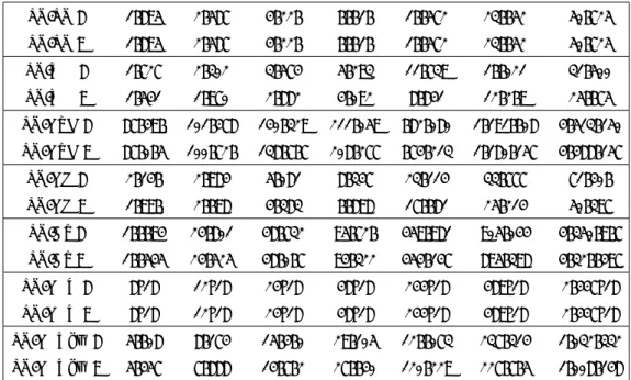
P arameters Distribution LogNormal W eibull GPD GH α -Stable GEV GEVbm µ 4.412992 -1541.558 -5.5846599 -587.855749 50.272385 σ 1.653022 -2137.940297 64.720971 α -0.5895611 -0.1906536 0.86700 -β -182.9008432 1185.8083087 0.1906304 0.95000 -ξ -0.9039617 -675 923 3.634536 1.030459 δ -22.5118547 58.18019 -λ --0.871847 -γ -54.21489 -KS < 2.2e-16 < 2.2e-16 < 2.2e-16 < 2.2e-16 < 2.2e-16 < 2.2e-16 < 2.2e-16 AD 6.117e-09 6.117e-09 6.117e-09 NA 6.117e-09 (d) 6.117e-09 6.117e-09 T able 1: This table pro vides the estimated parameters for the sev en parametric distributions fitted on the op erartional risk data set. If for the α stable distribution α < 1 , for the GEV, GEVbm and GPD ξ > 1 w e are in the presence of an infinite mean mo del. The p-v alu e s of b oth K olmogoro v-Smirno v and Anderson-Darling tests are also pro vided for the fit of eac h distribution.
X1 X2 LogNormal W eibull GPD GH Alpha-Stable GEV GEVbm V aR X1 ,X 2 E SX 1 ,X 2 V aR X1 ,X 2 E SX 1 ,X 2 V aR X1 ,X 2 E SX 1 ,X 2 V aR X1 ,X 2 E SX 1 ,X 2 V aR X1 ,X 2 E SX 1 ,X 2 V aR X1 ,X 2 E SX 1 ,X 2 V aR X1 ,X 2 E SX 1 ,X 2 LogNormal p1 2 493 6 103 2 328 4 820 75 546 217 916 2 618 7 753 2 552 44 407 2.834332e+07 1.721696e+21 2 658 19 225 p2 4 087 9 057 3 528 6 805 93 442 353 270 4 662 12 064 4 731 85 397 3.665483e+08 3.443392e+21 4 872 34 914 p3 7 252 14 693 5 735 10 419 142 038 716 560 9 291 20 539 10 725 203 193 1.072611e+10 8.608479e+21 10 723 76 829 p4 24 250 43 132 16 710 27 468 746 560 4 871 970 36 925 59 361 111 991 1 789 756 5.390204e+13 8.608479e+22 83 960 551 875 W eibull p1 -2 230 3 637 75 270 219 140 2 424 6 507 2 345 80 360 2.874992e+07 1.648438e+21 2 459 32 126 p2 -3 110 4 663 92 818 356 117 4 019 9 939 4 029 157 714 3.746901e+08 3.296876e+21 4 202 61 102 p3 -4 425 6 176 140 307 725 572 7 651 16 774 9 003 385 667 1.062522e+10 8.242191e+21 8 856 143 962 p4 -8 542 10 777 744 266 4 982 719 29 929 48 745 102 987 3 644 010 4.051415e+13 8.242191e+22 81 979 1 249 637 GPD p1 -150 276 481 590 75 882 198 596 76 003 253 293 2.900050e+07 8.175899e+21 2.852749e+07 8.991075e+20 p2 -185 210 799 161 93 953 314 173 94 929 423 142 3.804500e+08 1.635180e+22 3.719388e+08 1.798215e+21 p3 -281 725 1 667 960 143 016 618 297 149 135 886523 1.055955e+10 4.087950e+22 1.038451e+10 4.495538e+21 p4 -1 482 342 12 136 572 735 168 3 911 547 869 960 6 369 873 5.299107e+13 4.087950e+23 4.773943e+13 4.495538e+22 GH p1 -2 784 9 385 2 705 73 357 2.880134e+07 3.149731e+20 2.875817e+07 6.426626e+19 p2 -5 338 14 981 5 470 142 939 3.771517e+08 6.299462e+20 3.674012e+08 1.285325e+20 p3 -11 469 25 984 13 280 344 980 1.092553e+10 1.574866e+21 1.088133e+10 3.213313e+20 p4 -47 282 75 037 120 486 3 167 054 5.156340e+13 1.574866e+22 4.991674e+13 3.213313e+21 Alpha-Stable p1 -2 649 146 535 2.868921e+07 2.877576e+22 2 822 31 932 p2 -5 648 289 288 3.667449e+08 5.755152e+22 5 644 59 930 p3 -15 890 709 490 1.007457e+10 1.438788e+23 13 339 137 177 p4 -225 543 6 659 012 3.907140e+13 1.438788e+24 96 356 1 107 042 GEV p1 -1.822300e+08 1.096423e+28 2.875582e+07 1.635820e+19 p2 -2.615063e+09 2.192846e+28 3.640431e+08 3.271639e+19 p3 -8.028848e+10 5.482116e+28 1.075443e+10 8.179098e+19 p4 -4.437624e+14 5.482116e+29 4.820065e+13 8.179098e+20 GEVbm p1 -2 894 59 150 p2 -5 985 114 221 p3 -15 597 271 596 p4 -170 339 2 336 019 T able 2: Corre lated Risk Measures -this table presen ts the V aRs and the ESs ob tai n e d on fully correlated random v ariables sim ulated with sev e n distributions.
LN-LN 1 393 663 1, 373 2, 503 7, 721 11, 661 27, 292 LN-LN 2 395 667 1, 376 2, 503 7, 721 11, 677 27, 517 LN-WE 1 447 742 1, 439 2, 427 6, 299 8, 924 18, 498 LN-WE 2 564 826 1, 374 2, 068 4, 654 6, 406 14, 066 LN-GPD 1 4, 321 6, 181 11, 432 21, 158 88, 382 163, 788 689, 569 LN-GPD 2 58, 968 60, 766 65, 759 74, 945 138, 510 209, 859 726, 643 LN-GH 1 364 611 1, 313 2, 569 9, 882 16, 037 41, 329 LN-GH 2 480 742 1, 418 2, 528 8, 205 12, 765 30, 592 LN-AS 1 377 614 1, 269 2, 461 10, 965 21, 402 111, 987 LN-AS 2 476 725 1, 374 2, 472 9, 657 18, 319 101, 929 LN-GEV 1 25, 132 137, 464 2, 097, 977 28, 700, 959 10.73e9 134.51e9 47, 029e9 LN-GEV 2 25, 313 138, 221 2, 095, 098 29, 156, 891 10.47e9 135.38e9 45, 501e9 LN-GEVbm 1 366 614 1, 312 2, 579 11, 037 20, 542 91, 109 LN-GEVbm 2 481 742 1, 423 2, 571 9, 670 17, 603 80, 694
Table 3: The sum of VaR(X) and VaR(Y) (line 1) versus VaR(X + Y) (line 2) for couples of distributions: LN = lognormal, WE = Weibull, GPD = Generalised Pareto, GH = Generalised Hyperbolic, AS = Alpha-Stable, GEV = Generalised Extreme Value, GEVbm = Generalised Extreme Value calibrated on maxima. The percentiles represented are the 70th, 80th, 90th, 95th, 99th, 99.5th and 99.9th. We use the distributions fitted on the data set representing "Execution, Delivery, and process Management".
WE-WE 1 501 820 1, 505 2, 352 4, 878 6, 187 9, 703 WE-WE 2 501 821 1, 510 2, 352 4, 879 6, 185 9, 807 WE-GPD 1 4, 376 6, 259 11, 498 21, 082 86, 961 161, 051 680, 774 WE-GPD 2 58, 916 60, 639 65, 520 74, 662 138, 368 209, 701 726, 035 WE-GH 1 418 690 1, 379 2, 494 8, 460 13, 300 32, 534 WE-GH 2 533 795 1, 379 2, 208 6, 472 10, 534 27, 998 WE-AS 1 431 692 1, 335 2, 386 9, 544 18, 665 103, 193 WE-AS 2 528 779 1, 341 2, 148 7, 556 16, 025 101, 095 WE-GEV 1 25, 186 137, 542 2, 098, 044 28, 700, 884 10.73e9 134.51e9 47, 029e9 WE-GEV 2 25, 197 138, 107 2, 094, 946 29, 156, 852 10.47e9 135.38e9 45, 501e9 WE-GEVbm 1 420 692 1, 379 2, 504 9, 616 17, 805 82, 315 WE-GEVbm 2 534 796 1, 381 2, 237 7, 710 15, 281 79, 250
Table 4: The sum of VaR(X) and VaR(Y) (line 1) versus VaR(X + Y) (line 2) for couples of distributions: LN = lognormal, WE = Weibull, GPD = Generalised Pareto, GH = Generalised Hyperbolic, AS = Alpha-Stable, GEV = Generalised Extreme Value, GEVbm = Generalised Extreme Value calibrated on maxima. The percentiles represented are the 70th, 80th, 90th, 95th, 99th, 99.5th and 99.9th. We use the distributions fitted on the data set representing "Execution, Delivery, and process Management".
GPD-GPD 1 8, 250 11, 699 21, 490 39, 812 169, 044 315, 915 1, 351, 846 GPD-GPD 2 117, 080 120, 546 130, 394 148, 749 276, 271 418, 831 1, 452, 006 GPD-GH 1 4, 292 6, 129 11, 372 21, 224 90, 543 168, 164 703, 606 GPD-GH 2 59, 005 60, 888 66, 096 75, 538 139, 002 209, 869 726, 103 GPD-AS 1 4, 305 6, 131 11, 328 21, 116 91, 627 173, 528 774, 264 GPD-AS 2 58, 987 60, 890 66, 273 76, 314 147, 644 229, 984 834, 971 GPD-GEV 1 29, 061 142, 981 2, 108, 036 28, 719, 614 10.73e9 134.51e9 47, 029e9 GPD-GEV 2 92, 215 210, 767 2, 181, 852 29, 254, 626 10.47e9 135.38e9 45, 501e9 GPD-GEVbm 1 4, 292 6, 129 11, 372 21, 224 90, 543 168, 164 703, 606 GPD-GEVbm 2 59, 005 60, 888 66, 096 75, 538 139, 002 209, 869 726, 103 GH-GH 1 335 559 1, 253 2, 635 12, 043 20, 413 55, 366 GH-GH 2 335 559 1, 253 2, 635 12, 043 20, 413 55, 366 GH-AS 1 348 562 1, 209 2, 527 13, 126 25, 778 126, 024 GH-AS 2 442 683 1, 393 2, 778 12, 596 23, 446 104, 497 GH-GEV 1 25, 103 137, 412 2, 097, 918 28, 701, 025 10.73e9 134.51e9 47, 029e9 GH-GEV 2 25, 635 138, 429 2, 095, 206 29, 157, 735 10.47e9 135.38e9 45, 501e9 GH-GEVbm 1 336 562 1, 252 2, 645 13, 198 24, 917 105, 146 GH-GEVbm 2 446 703 1, 451 2, 895 12, 502 22, 224 84, 680
Table 5: The sum of VaR(X) and VaR(Y) (line 1) versus VaR(X + Y) (line 2) for couples of distributions: LN = lognormal, WE = Weibull, GPD = Generalised Pareto, GH = Generalised Hyperbolic, AS = Alpha-Stable, GEV = Generalised Extreme Value, GEVbm = Generalised Extreme Value calibrated on maxima. The percentiles represented are the 70th, 80th, 90th, 95th, 99th, 99.5th and 99.9th. We use the distributions fitted on the data set representing "Execution, Delivery, and process Management".
AS-AS 1 361 564 1, 165 2, 419 14, 210 31, 142 196, 682 AS-AS 2 360 562 1, 159 2, 428 14, 153 31, 459 201, 447 AS-GEV 1 25, 116 137, 414 2, 097, 873 28, 700, 918 10.73e9 134.51e9 47, 029e9 AS-GEV 2 26, 139 140, 091 2, 099, 977 29, 175, 188 10.47e9 135.38e9 45, 501e9 AS-GEVbm 1 349 564 1, 208 2, 537 14, 282 30, 282 175, 804 AS-GEVbm 2 443 683 1, 399 2, 849 15, 645 33, 285 189, 589 GEV-GEV 1 49, 871 274, 264 4, 194, 582 57, 399, 416 21.46e9 269e9 94, 058e9 GEV-GEV 2 49, 844 275, 821 4, 189, 583 58, 313, 419 20.94e9 271e9 91, 002e9 GEV-GEVbm 1 25, 105 137, 414 2, 097, 917 28, 701, 036 10.73e9 134.51e9 47, 029e9 GEV-GEVbm 2 26, 105 139, 855 2, 099, 195 29, 174, 309 10.47e9 135.38e9 45, 501e9 GEVbm-GEVbm 1 338 564 1, 252 2, 656 14, 353 29, 422 154, 927 GEVbm-GEVbm 2 340 565 1, 251 2, 663 14, 609 29, 967 158, 273
Table 6: The sum of VaR(X) and VaR(Y) (line 1) versus VaR(X + Y) (line 2) for couples of distributions: LN = lognormal, WE = Weibull, GPD = Generalised Pareto, GH = Generalised Hyperbolic, AS = Alpha-Stable, GEV = Generalised Extreme Value, GEVbm = Generalised Extreme Value calibrated on maxima. The percentiles represented are the 70th, 80th, 90th, 95th, 99th, 99.5th and 99.9th. We use the distributions fitted on the data set representing "Execution, Delivery, and process Management".
LN-LN 1 1, 895 2, 587 4, 226 6, 616 16, 572 23, 652 50, 725 LN-LN 2 1, 895 2, 587 4, 226 6, 616 16, 572 23, 652 50, 725 LN-WE 1 1, 727 2, 302 3, 574 5, 293 11, 739 16, 021 31, 500 LN-WE 2 1, 541 1, 970 2, 882 4, 092 8, 841 12, 269 25, 675 LN-GPD 1 87, 496 101, 478 140, 329 211, 059 682, 080 1, 191, 608 4, 513, 150 LN-GPD 2 87, 065 100, 726 138, 767 208, 277 674, 213 1, 180, 157 4, 488, 157 LN-GH 1 2, 146 2, 984 5, 081 8, 347 23, 114 33, 777 71, 406 LN-GH 2 1, 996 2, 698 4, 383 6, 898 17, 681 25, 214 50, 397 LN-AS 1 16, 694 24, 801 48, 732 95, 726 459, 981 905, 044 4, 350, 967 LN-AS 2 16, 545 24, 525 48, 067 94, 322 454, 147 895, 398 4, 326, 497 LN-GEV 1 8e18 12e18 24e18 48e18 244e18 489e18 2, 447e18 LN-GEV 2 8e18 12e18 24e18 48e18 244e18 489e18 2, 447e18 LN-GEVbm 1 5, 608 8, 174 15, 460 29, 105 126, 073 237, 314 1, 032, 332 LN-GEVbm 2 5, 457 7, 888 14, 762 27, 640 120, 229 227, 765 1, 008, 148
Table 7: The sum of ES(X) and ES(Y) (line 1) versus ES(X + Y) (line 2) for couples of distributions: LN = lognormal, WE = Weibull, GPD = Generalised Pareto, GH = Generalised Hyperbolic, AS = Alpha-Stable, GEV = Generalised Extreme Value, GEVbm = Generalised Extreme Value calibrated on maxima. The percentiles represented are the 70th, 80th, 90th, 95th, 99th, 99.5th and 99.9th. We use the distributions fitted on the data set representing "Execution, Delivery, and process Management".
WE-WE 1 1, 559 2, 016 2, 921 3, 970 6, 905 8, 390 12, 276 WE-WE 2 1, 559 2, 016 2, 921 3, 970 6, 905 8, 390 12, 276 WE-GPD 1 87, 328 101, 193 139, 676 209, 736 677, 247 1, 183, 977 4, 493, 926 WE-GPD 2 86, 887 100, 505 138, 515 208, 044 674, 087 1, 180, 072 4, 488, 101 WE-GH 1 1, 978 2, 698 4, 428 7, 024 18, 280 26, 146 52, 182 WE-GH 2 1, 810 2, 389 3, 739 5, 758 15, 192 22, 257 46, 312 WE-AS 1 16, 526 24, 516 48, 079 94, 403 455, 148 897, 413 4, 331, 742 WE-AS 2 16, 359 24, 217 47, 423 93, 172 452, 023 893, 523 4, 325, 897 WE-GEV 1 8e18 12e18 24e18 48e18 244e18 489e18 2447e18 WE-GEV 2 8e18 12e18 24e18 48e18 244e18 489e18 2447e18 WE-GEVbm 1 5, 440 7, 889 14, 807 27, 782 121, 240 229, 683 1, 013, 108 WE-GEVbm 2 5, 270 7, 579 14, 119 26, 506 118, 106 225, 770 1, 007, 256
Table 8: The sum of ES(X) and ES(Y) (line 1) versus ES(X + Y) (line 2) for couples of distributions: LN = lognormal, WE = Weibull, GPD = Generalised Pareto, GH = Generalised Hyperbolic, AS = Alpha-Stable, GEV = Generalised Extreme Value, GEVbm = Generalised Extreme Value calibrated on maxima. The percentiles represented are the 70th, 80th, 90th, 95th, 99th, 99.5th and 99.9th. We use the distributions fitted on the data set representing "Execution, Delivery, and process Management".
GPD-GPD 1 173, 097 200, 369 276, 431 415, 503 1, 347, 588 2, 359, 564 8, 975, 575 GPD-GPD 2 173, 097 200, 369 276, 431 415, 503 1, 347, 588 2, 359, 564 8, 975, 575 GPD-GH 1 87, 747 101, 874 141, 183 212, 791 688, 622 1, 201, 732 4, 533, 832 GPD-GH 2 87, 330 101, 092 139, 298 208, 887 674, 421 1, 180, 208 4, 488, 112 GPD-AS 1 102, 295 123, 692 184, 834 300, 169 1, 125, 489 2, 073, 000 8, 813, 392 GPD-AS 2 101, 891 122, 938 182, 933 295, 782 1, 098, 582 2, 016, 042 8, 499, 442 GPD-GEV 1 8e18 12e18 24e18 48e18 244e18 489e18 2, 447e18 GPD-GEV 2 8e18 12e18 24e18 48e18 244e18 489e18 2, 447e18 GPD-GEVbm 1 91, 209 107, 065 151, 562 233, 548 791, 581 1, 405, 270 5, 494, 758 GPD-GEVbm 2 90, 787 106, 267 149, 558 229, 042 766, 781 1, 355, 085 5, 243, 081 GH-GH 1 2, 397 3, 380 5, 935 10, 078 29, 655 43, 901 92, 088 GH-GH 2 2, 397 3, 380 5, 935 10, 078 29, 655 43, 901 92, 088 GH-AS 1 16, 945 25, 197 49, 586 97, 457 466, 523 915, 168 4, 371, 648 GH-AS 2 16, 809 24, 941 48, 924 95, 926 458, 199 899, 741 4, 327, 096 GH-GEV 1 8e18 12e18 24e18 48e18 244e18 489e18 2, 447e18 GH-GEV 2 8e18 12e18 24e18 48e18 244e18 489e18 2, 447e18 GH-GEVbm 1 5, 858 8, 571 16, 314 30, 836 132, 615 247, 439 1, 053, 014 GH-GEVbm 2 5, 722 8, 305 15, 616 29, 227 124, 294 232, 340 1, 009, 422
Table 9: The sum of ES(X) and ES(Y) (line 1) versus ES(X + Y) (line 2) for couples of distributions: LN = lognormal, WE = Weibull, GPD = Generalised Pareto, GH = Generalised Hyperbolic, AS = Alpha-Stable, GEV = Generalised Extreme Value, GEVbm = Generalised Extreme Value calibrated on maxima. The percentiles represented are the 70th, 80th, 90th, 95th, 99th, 99.5th and 99.9th. We use the distributions fitted on the data set representing "Execution, Delivery, and process Management".
AS-AS 1 31, 493 47, 015 93, 237 184, 836 903, 390 1, 786, 436 8, 651, 209 AS-AS 2 31, 493 47, 015 93, 237 184, 836 903, 390 1, 786, 436 8, 651, 209 AS-GEV 1 8e18 12e18 24e18 48e18 244e18 489e18 2, 447e18 AS-GEV 2 8e18 12e18 24e18 48e18 244e18 489e18 2, 447e18 AS-GEVbm 1 20, 406 30, 388 59, 965 118, 215 569, 482 1, 118, 706 5, 332, 574 AS-GEVbm 2 20, 270 30, 130 59, 302 116, 655 559, 704 1, 097, 691 5, 212, 237 GEV-GEV 1 16e18 24e18 48e18 97e18 489e18 979e18 4, 895e18 GEV-GEV 2 16e18 24e18 48e18 97e18 489e18 979e18 4, 895e18 GEV-GEVbm 1 8e18 12e18 24e18 48e18 244e18 489e18 2, 447e18 GEV-GEVbm 2 8e18 12e18 24e18 48e18 244e18 489e18 2, 447e18 GEVbm-GEVbm 1 9, 320 13, 761 26, 693 51, 593 235, 574 450, 977 2, 013, 940 GEVbm-GEVbm 2 9, 320 13, 761 26, 693 51, 593 235, 574 450, 977 2, 013, 940
Table 10: The sum of ES(X) and ES(Y) (line 1) versus ES(X + Y) (line 2) for couples of distributions: LN = lognormal, WE = Weibull, GPD = Generalised Pareto, GH = Generalised Hyperbolic, AS = Alpha-Stable, GEV = Generalised Extreme Value, GEVbm = Generalised Extreme Value calibrated on maxima. The percentiles represented are the 70th, 80th, 90th, 95th, 99th, 99.5th and 99.9th. We use the distributions fitted on the data set representing "Execution, Delivery, and process Management".
%tile Distribution Empirical LogNormal W eibull GPD GH Alpha-Stable GEV GEVbm V aR ES V aR ES V aR ES V aR ES V aR ES V aR ES V aR ES V aR ES 90% 575 2 920 686 2 090 753 1 455 10 745 146 808 627 2 950 582 29 847 + ∞ 2.097291e+06 + ∞ 626 12 755 95% 1 068 5 051 1 251 3 264 1 176 1 979 19 906 224 872 1 317 5 006 1 209 58 872 + ∞ 2.869971e+07 + ∞ 1 328 24 616 97 .5% 1 817 8 775 2 106 4 925 1 674 2 572 37 048 368 703 2 608 8 187 2 563 116 016 + ∞ 3.735524e+08 + ∞ 2 762 47 356 99% 3 662 18 250 3 860 8 148 2 439 3 468 84 522 758 667 5 917 14 721 7 105 283 855 + ∞ 1.073230e+10 + ∞ 7 177 111 937 99 .9% 31 560 104 423 13 646 24 784 4 852 6 191 675 923 5 328 594 28 064 46 342 98 341 2 649 344 + ∞ 4.702884e+13 + ∞ 77 463 945 720 T able 11: Univ ariate Risk Measures -This table exhibits the V aRs and ESs for the heigh t typ es of distributions considered -for instance empirical, lognormal, W eibull, GPD, GH, α -stable, GEV and GEV fitted on a series of maxima -for fiv e confidence lev el (for instance, 90%, 95%, 97.5%, 99% and 99.9%) ev aluated on th e p erio d 2009-2014. Note that th e parameters obtained for th e α -stable and the GEV fitted on the en tire data set lead to infinite mean mo d e l and therefore, the ES are hardly applicable.