HAL Id: hal-01143213
https://hal.inria.fr/hal-01143213
Submitted on 16 Apr 2015
HAL is a multi-disciplinary open access
archive for the deposit and dissemination of
sci-entific research documents, whether they are
pub-lished or not. The documents may come from
teaching and research institutions in France or
abroad, or from public or private research centers.
L’archive ouverte pluridisciplinaire HAL, est
destinée au dépôt et à la diffusion de documents
scientifiques de niveau recherche, publiés ou non,
émanant des établissements d’enseignement et de
recherche français ou étrangers, des laboratoires
publics ou privés.
Perfusion MRI Deconvolution with Delay Estimation
and Non-Negativity Constraints
Marco Pizzolato, Aurobrata Ghosh, Timothé Boutelier, Rachid Deriche
To cite this version:
Marco Pizzolato, Aurobrata Ghosh, Timothé Boutelier, Rachid Deriche. Perfusion MRI Deconvolution
with Delay Estimation and Non-Negativity Constraints. International Symposium on Biomedical
Imaging, Apr 2015, Brooklyn, New York, United States. �10.1109/ISBI.2015.7164057�. �hal-01143213�
Perfusion MRI Deconvolution with Delay Estimation and Non-Negativity Constraints
Marco Pizzolato
?Aurobrata Ghosh
?Timoth´e Boutelier
†Rachid Deriche
??
Athena Project-Team, Inria Sophia Antipolis - M´editerran´ee, France
†Olea Medical, La Ciotat, France
ABSTRACT
Perfusion MRI deconvolution aims to recover the time-dependent residual amount of indicator (residue function) from the measured arterial and tissue concentration time-curves. The deconvolution is complicated by the presence of a time lag between the measured concentrations. Moreover the residue function must be non-negative and its shape may become non-monotonic due to dispersion phenomena. We introduce Modified Exponential Bases (MEB) to perform de-convolution. The MEB generalize the previously proposed exponential approximation (EA) by taking into account the time lag and introducing non-negativity constraints for the recovered residue function also in the case of non-monotonic dispersed shapes, thus overcoming the limitation due to the non-increasing assumtion of the EA. The deconvolution prob-lem is solved linearly. Quantitative comparisons with the widespread block-circulant Singular Value Decomposition show favorable results in recovering the residue function.
Index Terms— Perfusion, Deconvolution, Exponential Bases, Delay, Dispersion, Non-Negative, DSC-MRI
1. INTRODUCTION
Perfusion imaging aims to recover parameters related to the passage of blood in the parenchyma (i.e. the functional part) of a tissue. The amount of perfusion is related to the function-ality of the parenchyma and its grade of activity.
The perfusion can be characterized in vivo using Dynamic Susceptibility Contrast MRI (DSC-MRI) where a bolus of paramagnetic contrast agent (PA) is injected in the subject’s vascular system. In each voxel, a signal related to the PA con-centration is acquired on a time sampling grid to derive the correspondent tissue concentration curve Cts(t). According
to the indicator-dilution theory [1], the measured Cts(t) in a
voxel is expressed as the convolution between the arterial in-put concentration to the voxel Ca(t), and a curve R(t) which
expresses at each time the residual amount of PA in the voxel
Cts(t) =
Z t
0
Ca(θ)R(t − θ)dθ (1)
The authors express their thanks to Olea Medical and to the Provence-Alpes-Cˆote d’Azur Regional Council for providing grant and support.
where R(t) is unknown and must be recovered from the ob-served Ca(t) and Cts(t) by means of deconvolution. The
quality of the reconstructed R(t) directly affects the estima-tion of the perfusion parameters such as the blood flow (BF), the blood volume (BV) and the mean transit time (MTT).
Since deconvolution is ill-posed [2] several regularization methods have been proposed to suppress noise, such as the truncated Singular Value Decomposition (tSVD) [3]. More recently a deconvolution method [2] based on exponential bases approximation (EA) showed to outperform tSVD by modeling R(t) as a weighted sum of exponentially decaying functions.
However those techniques show some limitations related to a technical issue inherent the perfusion data acquisition and the physiological nature of the residue function. In real prac-tice, indeed, it is impossible to measure the actual arterial con-centration in input to a specific voxel and normally Ca(t) is
selected as the tissue concentration of a voxel within a region containing only arterial blood. Therefore the concentrations Cts(t) of all the other voxels are physiologically delayed with
respect to the selected arterial input Ca(t), or can anticipate
it, causing the failure of the deconvolution due to the lack of causality assumptions. In addition, the bolus of PA may undergo dispersion which causes the shape of Ca(t) to
mod-ify, thus changing the natural decreasing shape of R(t) into a non-monotonic one [4]. Such a shape is sometimes con-sidered in myocardial perfusion applications [5]. Moreover, since R(t) expresses the time-dependent remaining quantity of PA in the voxel, negative values are non-physiological and need to be avoided. The EA does not take into account the time lag (delay) between Ca(t) and Cts(t). In addition it
does not consider dispersion effects since it cannot guaran-tee non-negativity unless the residue function is constrained to be monotonically decreasing [2].
We propose Modified Exponential Bases (MEB) allowing time delay estimation and a straight forward implementation of non-negativity constraints also in case of non-monotonic dispersed residue functions. We discuss an iterative linear implementation of the MEB and compare the results with the standard block-circulant formulation of tSVD [6], henceforth addressed as oSVD, which is insensitive to the delay and thus comparable with the proposed technique.
2. THE DECONVOLUTION PROBLEM
Assuming the tissue concentration Cts(t) and the arterial
one Ca(t) both measured on an equally spaced time grid
t1, t2, . . . , tM of size M , with ∆t = ti+1− ti, then Eq. 1 is
discretized as Cts(tj) = ∆t j X i=0 Ca(ti)R(tj− ti) (2)
which can be formulated in matrix form as cts = Ar, where
A is the M ×M convolution matrix containing the samples of the arterial input concentration, ctscontains the M samples of
the tissue concentration and r contains the M unknown sam-ples of the residue function. If a model R(t) = G(t, p) for the residue function is defined, then the deconvolution prob-lem is finding the set of parameters p. In case of linearity in the parameters the residue function can be written as r = Gp, where G is the M × N design matrix and p the N × 1 vector of coefficients with N ≤ M . Therefore the convolution is formulated as cts= AGp, where p is unknown.
In [2] it is proposed the exponential approximation (EA) to perform deconvolution, which searches a solution for R(t) in the span of decaying exponential functions, thus modeling the residue function as a sum truncated to an order N
R(t) =
N
X
n=1
kne−λntu(t) (3)
where u(t) is the Heaviside step function and the time rates λn are chosen according to the harmonic distribution
λn = n/T , with T the observation time interval. The
un-known parameters p = [k1, ..., kN] are found with R(t)
constrained to be at the same time non-negative R(t) ≥ 0 and non-increasing R0(t) ≤ 0 for t > 0, where the non-negativity holds due to the non-increasing assumption [2]. Therefore EA, in order to guarantee non-negativity, neglects dispersion effects assuming a non-increasing shape for R(t). In addition it does not take into account the time delay between Ca(t) and
Cts(t). In the following section we propose a more general
solution solving these limitations.
3. MODIFIED EXPONENTIAL BASIS
In order to estimate the time delay τ and guarantee the negativity for both monotonically decreasing and non-monotonic residue functions, we propose Modified Exponen-tial Bases (MEB). Each basis is constituted as the sum of an exponential decay and the opposite of its derivative with re-spect to the time rate, rere-spectively weighted by two different constants, anand bn. Each basis shape can thus vary between
a pure exponential decay (bn = 0) and its derivative term
(an= 0). Therefore the MEB include the EA and generalize
it by integrating the exponential derivative terms. Moreover
the time delay τ is explicitly considered with a Heaviside step function and is included in the exponentials, giving
R(t) = u(t − τ )
N
X
n=1
(an+ bn(t − τ ))e−αn(t−τ ). (4)
Hence, we can guarantee non-negativity just by constraining all the an and bn to be non-negative, and at the same time
recover both monotonically decreasing and non-monotonic convolution kernels.
The deconvolution problem incorporating Eq. 4 has a non-linear solution since the unknown αnand τ appear in the
ex-ponential. However the time rates αn can be preset without
loss of generality [2], thus allowing to find an iterative linear procedure to estimate the unknowns.
In order to fix the rates αn we found that the harmonic
rule proposed in [2] is too sensitive to the chosen maximum basis order N , as also reported in [7]. Despite such a rule can be used, we decide to calculate the rates based on the signal rather than the observation time interval. We define M T Tmax as the maximum M T T expected. This can be
fixed empirically, or set according to a conservative value calculated from the MTT found with mono-exponential ap-proximation or via oSVD. Then the time rates αn of Eq. 4
are calculated as the reciprocal of the M T T values harmon-ically distributed in the range [M T Tmin, M T Tmax] where
M T Tmin = M T Tmax/N .
In order to consider the delay τ in the estimation we no-tice that, due to the linearity of the convolution, it can be in-corporated in the residue function estimation. To account for this, the problem formulated in Sec. 2 must consider the circu-lar formulation of the convolution [6]. More precisely Cts(t)
and Ca(t) of length M are extended by zero-padding up to a
length L ≥ 2M to avoid aliasing. Then the new L×L squared circular convolution matrix Achas entries Aci,j= Ca(ti−j+1)
if j ≤ i and Ac
i,j = Ca(tL+i−j+1) if j > i. In the rest we
drop the superscript for clarity, Ac
i,j= Ai,j. The convolution
problem is then formulated as cts= AG(τ )p, where G(τ ) is
the L × 2N τ -dependent design matrix extended to the circu-lar time sampling grid, and p is the vector containing the 2N coefficients aiand bito be estimated. We perform the
estima-tion of τ via grid search over a range [τmin, τmax] seconds,
with a time step τs≤ ∆t. The set of estimated parameters ˆp
is obtained as the Least Squares solution subject to ai, bi≥ 0,
∀i = 1, ..., N when the estimated delay ˆτ is that minimizing ||cts− AG(τ )ˆp||22among all τ ∈ [τmin, τmax].
4. EXPERIMENTAL DESIGN
We test the performance of the compared methods with two synthetic datasets, one generated with a decreasing residue function and the other with a non-monotonic (dis-persed) one. In the first case we adopt the bi-exponential model Rbi−exp(t) = A · e−τ1t+ (1 − A) · e−τ2t, where
(a) SN R = 80.
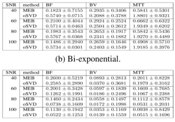
(b) Bi-exponential.
(c) Pharmacokinetic.
Fig. 1. Absolute relative error of estimates (mean and standard deviation).
τ1 = 0.68, τ2 = 0.05 and A = 0.95, according to the
nor-mal tissue values given in [8]. In the second case, we use the Pharmacokinetic model as formulated in [7], Rpk(t) =
(e−λ1t− e−λ2t)/(λ
2 − λ1) − (e−λ1t− e−λ3t)/(λ3 − λ1)
where we fix λ2 = 0.21, λ3 = 0.36 according to [5] and
λ1 = (λ3− λ2)/(M T T · λ2· λ3) with M T T ≈ 2.2 s, as
obtained from the bi-exponential model. We generate the actual residue function via multiplication of Rbi−exp(t) or
Rpk(t) with BF = 30 ml/100g/min, giving peak values of
BF for the bi-exponential model and ≈ 5.7 ml/100g/min for the pharmacokinetic one. In the latter case, the peak value will be considered as BF for the experiments. With the chosen parametrization, BV ≈ 1.1 ml/100g in all cases. The arterial concentration is generated according to [4] as Ca(t) = γ0(t−t0)ν·e−(t−t0)/βwith ν = 3, β = 1.5, γ0= 1,
and t0 = 30 s. The tissue concentration Cts(t) is then
ob-tained via Eq. 2. The concentration curves are then converted to signal intensities according to S(t) = S0· e−κ·C(t)·T E,
where T E is the echo time and κ is the susceptibility con-stant fixed according to [3]. We choose S0and T E separately
for the tissue concentration S0t = 200, T Et = 55 ms and
for the arterial one Sa0 = 600, T Ea = 13 ms, according to
[9]. The signals, obtained with repetition time ∆t = 1 s, are then corrupted with Gaussian noise with zero mean and standard deviation σ = S0/SN R, and finally reconverted in
concentration curves.
We performed the experiments separately for Cts(t)
ob-tained after convolution of Ca(t) with both the bi-exponential
and the pharmacokinetic kernel. In each case we delayed Ca(t) and Cts(t) with integer values in range [−5, 5]
sec-onds. For each delay we calculated the residue function via oSVD (20%) and MEB (N = 30, harmonic αn, M T Tmax=
4 · M T ToSV D, τmin = −10 s, τmax = 15 s, τs = 0.25 s)
deconvolution, and obtained the estimates of BF , BV and M T T . We tested four SN R values [9], [40, 60, 80, 100], gen-erating 100 noisy repetitions for each possible combination of kernel, delay and SN R.
(a) Pharmacokinetic kernel (b) fitting, SN R = 80
(c) Bi-exponential kernel (d) fitting, SN R = 80
Fig. 2. Residual error (a,c) and residue function fitting (b,d).
5. RESULTS AND DISCUSSION
Figure 1(a) illustrates the mean absolute relative error in the estimation of each parameter for the representative case of SN R = 80. Figures 1(b) and 1(c) show the tables giving the estimates mean errors and standard deviations for all the SN R, in the case of bi-exponential and pharmacokinetic kernel respectively. For both oSVD and MEB, we computed the mean residual error of the recovered residue function with respect to the ground truth, as shown in Fig. 2(a) and 2(c), for increasing noise levels, in case of dispersed and the bi-exponential kernel respectively; the std areas are shown. Fig. 2(b) and 2(d) show examples of the correspondent MEB and oSVD fittings against the ground truth.
We notice that, for both MEB and oSVD, the quality of the estimated parameters depends on the chosen convolution kernel (Fig. 1). In the case of a smooth kernel, such as the pharmacokinetic one, the MEB show less effective results than oSVD in estimating the parameters (table. 1(c)). Indeed oSVD cuts the high frequency oscillations of Ca(t) which, in
such a case, mainly correspond to noise. A possible explana-tion of the MEB performance is that the delay estimaexplana-tion is harder on the dispersed kernel due to its smoothness. Indeed, we found that the delay estimation error for the pharmacoki-netic kernel doubles that obtained for the bi-exponential one (≈ 42% against ≈ 19%, SN R = 80).
On the other hand oSVD show major limitations in the case of bi-exponential residue function. For instance the es-timation error of M T T almost doubles the magnitude of the correspondent ground truth value. This performance drop of oSVD is highly related to the marked underestimation of BF , with an error around the 57% of the actual blood flow as shown in Fig. 1(a) and in table 1(b).
The MEB outperform oSVD for the bi-exponential residue function as shown in Fig. 1(a) and in table 1(b). Indeed the MEB manage to reduce the underestimation of BF giving an average relative error in a range [15%, 21%] of the ground truth value. The MEB also allow to obtain an error for M T T always at least three times smaller than that of oSVD. The calculation of BV as the analytical integral of R(t) obtained via MEB is comparable to that obtained via oSVD. However it is normally preferable to estimate BV directly from the concentration curves Ca(t) and Cts(t) to avoid introducing
errors related to the deconvolution procedure.
The MEB show less residual error then oSVD for both of the tested kernels and at any SN R, as shown in Fig. 2(a) for the dispersed residue function and 2(c) for the bi-exponential one. We further notice that the MEB fitting is more robust to noise. Indeed Fig. 2(a) shows that with dispersed residue function, the difference between the oSVD residual error at SN R = 40 and SN R = 100 is almost four times higher than the correspondent difference for the MEB. The fitting capability of the MEB is more marked for the bi-exponential kernel, Fig. 2(c), where the amount of residual error stands between the 35% and the 60% of the oSVD error for any SN R. In general, the residue function recovered via MEB looks smoother and without ripples, which are a contributing cause to the oSVD residual error.
6. CONCLUSIONS
We introduced Modified Exponential Bases to perform per-fusion deconvolution. The proposed MEB generalize the exponential approximation by including both exponentially decaying terms and their derivatives. Indeed the MEB allow to take into account residue functions which are either purely decreasing or dispersed, providing at the same time a straight forward implementation of non-negativity constraints. The
MEB also explicitly take into account the time delay be-tween the arterial and the tissue concentrations. The oSVD showed a lower error in the perfusion parameters estimation for the dispersed residue function, in agreement with the lat-ter’s smoothness. However, in the case of the bi-exponential kernel the MEB outperform oSVD. In addition, for any type of kernel, the fitting results of the MEB compare favorably with respect to those obtained via oSVD, and are more ro-bust to noise. We believe that time delay estimation and non-negativity constraints help in recovering a physiologi-cally meaningful residue function. Moreover we find that performing deconvolution with continuous basis functions improves the robustness to noise and we think that proposed bases should take into account the variability in the possible shapes of the residue function.
7. REFERENCES
[1] Meier et al., “On the theory of the indicator-dilution method for measurement of blood flow and volume,” J Appl Physiol, vol. 6(12), pp. 731–744, 1954.
[2] Keeling et al., “Deconvolution for dce-mri using an ex-ponential approximation basis,” Med Image Anal, vol. 13(1), pp. 80–90, 2009.
[3] Østergaard et al., “High resolution measurement of cere-bral blood flow using intravascular tracer bolus passages. part i: Mathematical approach and statistical analysis,” Magn Reson Med, vol. 36(5), pp. 715–725, 1996.
[4] Calamante et al., “Delay and dispersion effects in dy-namic susceptibility contrast mri: simulations using sin-gular value decomposition,” Magn Reson Med, vol. 44(3), pp. 466–473, 2000.
[5] Zarinabad et al., “Voxelwise quantification of myocardial perfusion by cardiac magnetic resonance,” Magn Reson Med, pp. 1994–2004, 2012.
[6] Wu et al., “Tracer arrival timinginsensitive technique for estimating flow in mr perfusionweighted imaging using singular value decomposition with a blockcirculant de-convolution matrix,” Magn Reson Med, vol. 50(1), pp. 164–174, 2003.
[7] Batchelor et al., “Arma regularization of cardiac perfu-sion modeling,” ICASSP, pp. 642–645, March 2010.
[8] Mehndiratta et al., “Modeling the residue function in dscmri simulations: Analytical approximation to in vivo data,” Magn Reson Med, 2013.
[9] Wirestam et al., “Wavelet-based noise reduction for improved deconvolution of time-series data in dynamic susceptibility-contrast mri,” Magn Reson Mater Phy, vol. 18(3), pp. 113–118, 2005.