Publisher’s version / Version de l'éditeur:
Vous avez des questions? Nous pouvons vous aider. Pour communiquer directement avec un auteur, consultez la première page de la revue dans laquelle son article a été publié afin de trouver ses coordonnées. Si vous n’arrivez pas à les repérer, communiquez avec nous à [email protected].
Questions? Contact the NRC Publications Archive team at
[email protected]. If you wish to email the authors directly, please see the first page of the publication for their contact information.
https://publications-cnrc.canada.ca/fra/droits
L’accès à ce site Web et l’utilisation de son contenu sont assujettis aux conditions présentées dans le site LISEZ CES CONDITIONS ATTENTIVEMENT AVANT D’UTILISER CE SITE WEB.
Research Report (National Research Council of Canada. Institute for Research in
Construction), 2002-11-01
READ THESE TERMS AND CONDITIONS CAREFULLY BEFORE USING THIS WEBSITE. https://nrc-publications.canada.ca/eng/copyright
NRC Publications Archive Record / Notice des Archives des publications du CNRC : https://nrc-publications.canada.ca/eng/view/object/?id=246976fd-f98b-471d-a611-4f83cfb53e0f https://publications-cnrc.canada.ca/fra/voir/objet/?id=246976fd-f98b-471d-a611-4f83cfb53e0f
NRC Publications Archive
Archives des publications du CNRC
For the publisher’s version, please access the DOI link below./ Pour consulter la version de l’éditeur, utilisez le lien DOI ci-dessous.
https://doi.org/10.4224/20378449
Access and use of this website and the material on it are subject to the Terms and Conditions set forth at
FIERAsystem Enclosed Pool Fire Development Model: Theory Report
Kashef, A.; Bénichou, N.; Torvi, D. A.; Raboud, D. W.; Hadjisophocleous, G.
V.; Reid, I.
FIERAsystem Enclosed Pool Fire Development Model: Theory
Report
Kashef, A.; Bénichou, N.; Torvi, D.;
Raboud, D.W.; Hadjisophocleous, G.; Reid, I.
IRC-RR-121
November 2002
FIERAsystem Enclosed Pool Fire Development Model: Theory
Report
Ahmed Kashef, Noureddine Benichou, David Torvi, Don W. Raboud, George Hadjisophocleous and Irene Reid
Research Report #121
November 2002
Fire Risk Management Program Institute for Research in Construction National Research Council Canada
TABLE OF CONTENTS
TABLE OF CONTENTS... i
NOMENCLATURE... ii
1. INTRODUCTION... 4
2. ENCLOSED POOL FIRES... 5
2.1 CLASSIFICATION OF ENCLOSED POOL FIRES... 5
2.2 HEAT RELEASE RATES OF ENCLOSED POOL FIRES... 7
2.2.1 Peak Heat Release Rate of Enclosed Pool Fires – Fuel Controlled Fire... 7
2.2.2 Peak Heat Release Rate of Enclosed Pool Fires – Ventilation Controlled Fire... 8
2.3 DURATION AND DIAMETER OF ENCLOSED POOL FIRES... 9
2.3.1 Continuous, Unconfined Pool Fire... 9
2.3.2 Instantaneous, Unconfined Pool Fire... 10
2.3.3 Confined Pool Fires... 11
2.4 HEIGHT OF FLAME ABOVE POOL FIRE... 11
3. HEAT TRANSFER FROM POOL FIRES... 12
3.1 THERMAL RADIATION HEAT FLUXES... 12
3.2 CONVECTIVE HEAT FLUXES... 13
3.3 CRITICAL TIME FOR OCCUPANT RESPONSE, EVACUATION AND LIFE HAZARD MODELS... 14
4. REFERENCES... 15
APPENDIX A – VIEW FACTOR CALCULATIONS... 16
NOMENCLATURE
Notation
A area (m2)
cp constant pressure specific heat (J/kg⋅°C)
D diameter (m) E energy (kJ)
F radiation view factor
g acceleration due to gravity (9.81 m/s2) H height (m)
k factor for openings m mass burning rate (kg/s)
m” mass burning rate per unit area (kg/m2⋅s)
Q heat release rate (kW) q" heat flux (kW/m2) r radius (m)
S experimentally determined parameter SF safety factor
T temperature (°C) t time (s)
V volume (m3) v burning rate (m/s)
vL volume burning rate (m3/s)
W width (m) X distance (m) Z depth (m)
Greek Letters
α coefficient for a t2 fire
∆HC heat of combustion (kJ/kg) ∆Hv heat of vaporization (kJ/kg)
kβ mean beam length corrector extinction coefficient product (m-1).
η combustion efficiency
θ angle
ρ density (kg/m3)
τ atmospheric transmissivity, non-dimensional time
Subscripts a air amb ambient b boiling C combustion c ceiling, compartment cr critical dike dike e effective, emissive ep effective plume eq equivalent f fire, flame, fuel FC fuel controlled fo flashover
L liquid m maximum, modified o opening p peak, plume pool pool s spill S smoky T total
v vaporization, portion that can be viewed VC ventilation controlled
1. INTRODUCTION
As Canada and other countries move from prescriptive-based building codes to performance/objective-based codes, new design tools are needed to demonstrate that compliance with these new codes has been achieved. One such tool is the computer model FiRECAM™, which has been developed over the past decade by the Fire Risk Management Program of the Institute for Research in Construction at the National Research Council of Canada (NRC). FiRECAM™ is a computer model for evaluating fire protection systems in residential and office buildings that can be used to compare the expected safety and cost of candidate fire protection options.
To evaluate fire protection systems in light industrial buildings, a new computer model is being developed. This model, whose current focus is aircraft hangars and warehouses, is based on a framework that allows designers to establish objectives, select fire scenarios that may occur in the building and evaluate the impact of each of the selected scenarios on life safety, property protection and business interruption. The new computer model is called FIERAsystem, which stands for Fire Evaluation and Risk Assessment system.
FIERAsystem uses time-dependent deterministic and probabilistic models to evaluate the impact of selected fire scenarios on life, property and business interruption. The main FIERAsystem submodels calculate fire development, smoke movement through a building, time of failure of building elements and occupant response and evacuation. In addition, there are submodels dealing with the effectiveness of fire suppression systems and the response of fire departments.
In FIERAsystem, fire development models are used to simulate selected fire
scenarios. Each model has its own user interface and is designed as a stand-alone module. These models can also be used in conjunction with other FIERAsystem models in order to conduct a complete hazard or risk analysis. In the latter case, the fire development models provide information that will be subsequently used to determine the spread of fire between compartments and calculate the effects of selected fire scenarios on occupants, the building and its contents. For example, the Life Hazard Model [1] uses heat fluxes at various
distances from the fire to determine the probability of death due to high heat fluxes in an individual compartment in the building.
This report describes the theory of the Enclosed Pool Fire Development Model. The choice to use this particular model is made by the user, based on their knowledge of the building being evaluated and its occupancy, fuel loads, etc. The model calculates the quantities, which characterize the fire (heat release rate, temperature and thermal radiation heat fluxes) as a function of time. The equations used are taken from The SFPE Handbook of Fire Protection Engineering [2] and SINTEF’s Handbook for Fire Calculations and Fire Risk Assessment in the Process Industry [3]. The user should consult these references for information on the assumptions and limitations inherent in these equations before using this model.
2. ENCLOSED POOL FIRES
A pressurised release of either vapour or two-phase mixture may result in a fire whereas the momentum from a liquid release is more likely to be destroyed, and the release will form a pool fire. A pool fire is a type of turbulent diffusion flame, which burns above a pool of vaporising fuel where the fuel vapour has negligible initial momentum.
Many industrial fires involve hydrocarbon fuels. Depending on the release rate and ignition of these fuels, various types of gas or liquid pool fires may occur. Event trees, which provide guidance as to which type of fire will occur for a given set of ignition and release conditions, can be found in fire protection engineering handbooks (e.g. references 2, 3, 4). These references should be consulted to determine the suitability of the enclosed pool fire development models described in this report for a specific application. The model
calculations involve the estimation of fuel mass burning rate, flame shape parameters, view factor, and contours of incident heat flux.
2.1 Classification of Enclosed Pool Fires
An enclosed pool fire can be classified as either confined or unconfined. A confined pool fire is one in which there is a dike or other barrier that does not allow the fuel to spread beyond a certain diameter, whereas an unconfined pool fire is a fire where there is no barrier to prevent the fuel from spreading. Pool fires may also be classified on the basis of the rate and duration of the spill of fuel that burns. An instantaneous pool fire is a fire in which the spill of fuel occurs in a very short period of time, while a continuous pool fire is a fire in which the spill of fuel occurs at a given rate for a relatively long period of time. The distinction between “short time” and “long time” relays on different factors such as spill size, liquid properties, and ambient conditions. A non-dimensional critical time (τcr) is used to determine
whether the pool fire is continuous or instantaneous, and is calculated using the following expression [5]: 3 1/ L f s cr V v t = τ (1) Where:
ts = the duration of the spill (s);
νf = the maximum (infinite) burning rate of the fuel (m/s); and
VL = the total volume of fuel spilled (m3).
The pool fire is considered to be instantaneous if τcr < 0.002; otherwise, it is considered to
be continuous [5]. The burning rate used in Equation 1 is the infinite burning rate, which is independent of the diameter of the liquid pool.
The burning rate for a particular fuel has been found to vary with the pool diameter and can be calculated from the following correlation [5]:
(
k D)
ffi v e
v = 1− −β (2)
Where:
D = pool fire diameter (m);
νfi = the actual burning rate of the fuel (m/s); and
kβ = mean beam length corrector extinction coefficient product (m-1).
It can be noted that the burning rate, νfi, approaches the maximum burning rate at
large diameters. Burning rate may be calculated by dividing the mean heat flux from the fire to the pool by the heat of vaporization of the liquid. The mean heat flux includes the
conductive heat transfer rate through the pan rim the convective heat flux and the radiative heat transfer. The contributions of the conduction and convection heat transfer mechanisms to the total heat flux significantly decrease for pool diameters greater than a few centimetres [6], which is the case for most of the pool fires. Thus for most liquid fuels, the radiative heat transfer dominates the heat flux to the pool and it increases as the diameter increases. For large, radiation-dominated pool fires (pan diameters of about 1-3 m), the burning rates are essentially dependent on the thermodynamical properties of the liquid fuel (kβ). The burning rates of these types of fires can be calculated using the following equation [3]:
− + = − ) T T ( c H H ) ( . v f b p V C f ∆ ∆ 6 10 27 1 (3) Where:
∆HC = the heat of combustion of the fuel (kJ/kg); ∆Hv = the heat of vaporization of the fuel (kJ/kg);
cp = the specific heat of the fuel (kJ/kg⋅°C);
Tb = the boiling temperature of the fuel (°C); and
Tf = the fuel temperature (assumed to be the ambient temperature) (°C).
The numerator in Equation 3 can be viewed as the modified heat of vaporization and for a liquid above its boiling point it can be assumed to be equal to the heat of vaporization of the fuel at its boiling point.
The mass burning rate per unit area, mf”, can be calculated from the burning rate by
multiplying it by the liquid density of the fuel at its boiling point.
ρ ⋅ = f f" v m (4) Where:
mf” = fuel mass burning rate per unit area (kg/m2⋅s).
2.2 Heat Release Rates of Enclosed Pool Fires
The heat release rate of an enclosed pool fire at any time is calculated by assuming that the pool fire can be described as a t2 fire, using the following equation [7]:
2 t ) t ( Q =α (5) Where:
Q = the heat release rate of the fire at any time (kW); and
α = the fire growth coefficient (kW/s2).
This heat release rate is limited to the maximum heat release rate possible based on either the amount of fuel in the compartment or the oxygen that can be supplied to the fire from the compartment and through ventilation openings. The calculations used to determine the maximum heat release rate for either of the two cases are described in the following sections.
The value of the fire growth coefficient in Equation 5 depends on whether the pool fire is confined or unconfined. For a confined pool fire, where the diameter is assumed constant, an ultra-fast t2 fire is assumed and α has a value of 0.1876 kW/s2. The peak (or maximum) heat release rate, Qp, will then occur for times greater than tp, where:
1876 0.
Q
tp = p (6)
For an unconfined pool fire, α is chosen such that the maximum heat release rate occurs at the time, tm, when the diameter reaches its maximum value (see Equations 10 and
14), as follows: 2 m p t Q = α (7)
2.2.1 Peak Heat Release Rate of Enclosed Pool Fires – Fuel Controlled Fire
The peak heat release rate based on the quantity of available liquid fuel is calculated in the following manner [3]. First, the area of the liquid pool fire (Apool) is calculated:
4 2 m pool D A = π (8)
Where: Dm is the maximum diameter in m.
Next, the fuel mass-burning rate is calculated:
" m A
Where mf is the fuel burning rate (kg/s); and
The maximum fuel controlled heat release rate is then calculated using the following equation: c f FC m H Q =η ∆ (10) Where:
QFC = fuel controlled heat release rate (kW);
η = combustion efficiency (non-dimensional, 0 ≤η≤ 1, assumed to be 0.65 [8]); and
∆Hc = heat of combustion of the fuel (kJ/kg).
2.2.2 Peak Heat Release Rate of Enclosed Pool Fires – Ventilation Controlled Fire
Equation 10 calculates the heat release rate if the fire is controlled solely by the quantity of fuel in the compartment. This heat release rate is compared to the maximum heat release rate for a ventilation-controlled fire in the compartment. The calculation of the ventilation-controlled heat release involves the estimation of the air supply rate into the compartment. For a compartment with n openings with height Ho and width Wo, the air
supply rate is given by the following expression [3]:
(
)
e n i o o i a k W H H m = ∑ =1 (11) Where:ma = the mass flow rate of air supplied to the compartment (kg/s);
k = is a factor for openings;
= 0.5 for normal sized openings (e.g. windows, doors etc.);
= 0.13 for openings with either a height or width of greater than 5 m; and
He = effective opening height for multiple openings given by:
(
)
(
)
∑ ∑ = = = n i o o i n i i / o o e H W H W H 1 1 2 3 (12)For a single opening, Equation 11 reduces to:
2 3/ o o a kW H m = (13)
The maximum heat release rate for a ventilation-controlled fire, QVC is then
calculated using the following equation, which is valid for most fuels [8]:
a
VC m
The maximum heat release rates for the fuel- (Equation 10) and ventilation-controlled (Equation 14) scenarios are compared and the smaller of these two values is used as the peak heat release rate in the subsequent calculations. If the fire is ventilation-controlled, then the duration of the pool fire is adjusted using the following equation:
VC FC FC f VC f Q Q t t − = − (15) Where:
tf-VC = duration of a ventilation-controlled pool fire (s); and
tf-FC =duration of a fuel-controlled pool fire (s); using Equations 16, 21 or 24.
In other words, if the ventilation-controlled heat release rate is 50% of the fuel controlled ventilation heat release rate, the fire will last twice as long. For simplicity, this calculation has assumed that no fuel has been vaporized and leaves the compartment (i.e., all the fuel must be burned within the compartment).
2.3 Duration and Diameter of Enclosed Pool Fires
The diameter of the pool fire depends on a number of factors including the mode and rate of the release and the fuel-burning rate. This section deals with the procedure for calculating the duration and diameter of enclosed pool fires.
2.3.1 Continuous, Unconfined Pool Fire
For a continuous pool fire, the duration of the fire, tf-FC is simply the duration of the
spill (ts) (to be specified by the user). In other words:
s FC
f t
t − = (16)
The model assumes that the diameter of a pool fire increases linearly with time from 0.3 m to the maximum diameter, Dm. The maximum diameter of an unconfined pool fire is
assumed to be its equilibrium diameter, where the burning rate of the fuel is the same as the rate at which fuel is being spilled. Assuming that the dominant mode of heat transfer to the liquid pool comes from the flame and that the burning rate is constant, the maximum diameter is calculated using the following equation [5]:
2 1 2 / f L m v v D = π (17) Where: s L L t V v = (18)
VL volume of the fuel spill (m3);
The assumption that the initial diameter of the fire is 0.3 m is based on calculating the diameter for which a heat flux of 140 kW/m2 is predicted using a simple point source
representation of a 100 kW fire, which is 40% radiative.
pq"(t) (t) fQ D max 140 = (19) Where:
f = radiative fraction of the total heat release rate (user-specified); and
Qmax(t) = maximum heat release rate (kW); and
q”(t) = maximum flame heat flux (kW/m2) = 140 kW/m2
While the point source model generally underpredicts heat fluxes relatively close to a fire, it still provides a simple method of ensuring that the nominal diameter is realistic for the particular fire being modeled.
A 100 kW fire is about the size of a fire in a small wastepaper basket. This is thought to be a good estimate of the initial size of any fire that would be of interest to the engineers using FIERAsystem.
The assumption that the diameter increases linearly with time is based on the fact that the maximum fuel-controlled heat release rate of a fire is a function of the area of the fire, which is a function of the square of the diameter of the fire. Therefore, as a t2 fire
assumes that the heat release rate is a function of the square of the elapsed time, it follows that the diameter will be a linear function of time for a t2 fire.
The time required to reach this maximum diameter, tm, is given by [5]:
(
)
1 3 564 0 / m f m m D gv D . t = (20)Where: g is the acceleration due to gravity (m2/s).
2.3.2 Instantaneous, Unconfined Pool Fire
The duration of instantaneous unconfined pool fire is assumed to be the time
required for the fire to reach its maximum diameter, when almost all of the fuel is consumed, and is calculated using the following equation [3]:
4 1/ f L FC f gv V 0.6743 t = − (21)
Again, the model assumes that the diameter of the pool fire increases linearly with time from 0.3 m to the maximum diameter, Dm, which can be calculated from [3]:
v g V D / f L m 8 1 2 3 2 = (22)
2.3.3 Confined Pool Fires
The duration of a confined pool fire is calculated using the volume of fuel burned, the dike area and the burning rate of the fuel (all are specified by the user). First, the depth of fuel burned in the dike, Z is calculated using the following equation:
dike L
A V
Z = (23)
Where: Adike is the area of the dike (m2). Equation 23 uses the amount of fuel burned, not
just the amount of the spilled fuel. It is assumed that if the amount of fuel burned is greater than the amount that fits in the area of the dike, the excess fuel will be spilled slowly enough that this excess fuel burns as it is spilled. The duration of the fire is then calculated using:
f FC f v Z t − = (24)
The model assumes that the diameter of a confined pool fire increases linearly with time from 0.3 m to the maximum diameter, Dm. Dm is entered by the user for a circular dyke,
or is calculated as the diameter of an equivalent circular area for the case of a noncircular dyke, as follows: 2 1 4 dike / m A D = π (25)
2.4 Height of Flame above Pool Fire
The height of the flames above the pool fire at any time is calculated using Thomas’ correlation [5]: 61 0 42 . f f ) t ( gD " m ) t ( D ) t ( H ⋅ = ρ (26)
The flame height calculated using Equation 26 is compared with the height of the compartment, and a height of 1 m, which is assumed to be the height of the midsection of a person. The flame height is set to the height of the compartment if the height of the flame is greater than that of the compartment. The flame height is set to 1 m if the calculated height of the flame is less than this value.
3. HEAT TRANSFER FROM POOL FIRES
Heat transfer from pool fires includes both thermal radiation heat transfers from the flames to the surrounding objects as well as convection heat transfer. Convection heat transfer from the flames to engulfed objects is important particularly in calculating the response of boundaries to the fire.
3.1 Thermal Radiation Heat Fluxes
The heat fluxes from the pool fire to points, at various distances, located on a plan at an elevation of 1.0 m are calculated using the solid two-zone flame model of Mudan and Croce [6]. The model assumes that the visible portion of the flame emits a relatively high amount of thermal radiation, while the invisible gases do not emit a significant amount of thermal radiation. The following equation is used to calculate thermal radiation heat fluxes,
q”(t), at a distance from the fire.
SF ) t ( F " q ) t ( " q = e τ (27) Where:
q”e = emissive power of the pool fire (kW/m2);
) e (1 E e E " qe = m −SD(t)+ S − −SD(t) (28)
Em = maximum emissive power of the visible portion (kW/m2) ≅ 140;
ES = maximum emissive power of the smoky portion (kW/m2) ≅ 20;
S = experimentally determined parameter (m-1) = 0.12 m-1;
F(t) = view factor (see Appendix A)
τ = atmospheric transmissivity (1.0 considering relatively short distances); and
SF = safety factor (default value = 1).
A height of 1 m was chosen so as to be representative of the midsection of a person. The lower, highly-emitting portion of the fire, is assumed to have an emissive power of 140 kW/m2, while the upper, lower-emitting portion is assumed to have an emissive power of 20 kW/m2. Equation 27 was developed to estimate the average emissive power of large, sooty hydrocarbon fires using experimental data reported in the literature. Based on Equation 27, the average emissive power of a pool fire with a diameter of 1 m is predicted to be 126 kW/m2. If the pool diameter is increased to be 100 m, the emissive power is estimated to decrease to 20 kW/m2.
At each time step, the heat flux from the pool fire is calculated at the outside of each of 10 rings located from the centre of the room to the boundary of the compartment. These heat fluxes are used by the Life Hazard Model [1] to calculate the probability of death from exposure to high heat fluxes at each of the locations. The first ring is located at the
maximum diameter of the pool fire and the last ring is located at the equivalent boundary of a circular compartment representing the compartment being considered. In order to simplify these calculations, the time-dependence of the diameter during the earlier portion of the fire
is ignored. Within the maximum diameter of the fire, the heat flux is assumed to be equal to 140 kW/m2, the emitting power of the visible portion of the flame used in Equation 27.
For a non-circular compartment, the equivalent compartment diameter (Deq-c) is
calculated using the following equation:
π c c eq A D − = 4⋅ (29)
Where: Ac is the area of the compartment (m2).
3.2 Convective Heat Fluxes
In order to calculate the convective heat fluxes from the fire to the boundaries of the compartment, the temperature of the pool fire and the hot gas layer at the top of the
compartment are calculated. First the temperature at the centreline of the visible portion of the flame (Tf) is assumed to be 980°C and the emissivity of the fire is assumed to be 1.0.
This temperature and emissivity correspond to the thermal radiation heat flux of 140 kW/m2 assumed earlier for the visible portion of the flame.
The ceiling impingement temperature (Tc) at any time is calculated using the
following equation [9]: 5/3 c 2/3 amb c H (kQ(t)) 0.22 T (t) T = + (30) Where:
Tamb(t) = the ambient temperature (°C);
Q(t) = the heat release rate of the fire at any time (kW)
k = a factor to take into account is the effect of the compartment walls on the temperature of the hot plume gases;
= 1 (if no walls are nearby);
= 2 (if the fire is close to one wall – default value); = 4 (if the fire is in a corner); and
Hc = the compartment height (m).
Alpert and Ward [9] state that Equation 29 is derived from empirical data and is not valid when the flames are either very close to the ceiling or much farther away from the ceiling; therefore, it cannot predict temperatures greater than 825°C accurately. Therefore, if the temperature predicted by Equation 29 is greater than the 980°C temperature assumed for the flames, the model limits the ceiling impingement temperature to 980°C.
Effective Plume temperatures based on the flame and ceiling impingement
temperatures are then sent to the Building Element Failure Model [10] in order to determine the heat transfer to the boundaries and the time of failure of these boundaries. Details of how these equivalent temperatures are calculated can be found in Appendix B.
3.3 Critical Time for Occupant Response, Evacuation and Life Hazard Models
The Occupant Response, and Evacuation [11] and Life Hazard Models [1] require a critical time, which is the time after which occupants will be unable to evacuate the
compartment. As one of the possible values of this critical time, the fire development model calculates the time required for flashover to occur, using Thomas’ flashover correlation [8].
e o T fo . A A H Q =78 +378
(31) Where:
Qfo = heat release rate at flashover (kW);
AT = total surface area of the compartment (m2);
Ao = total area of openings (m2); and
He = equivalent height of openings (m).
The time to flashover is determined by comparing the time-dependent heat release rate data calculated earlier with the heat release rate necessary for flashover.
4. REFERENCES
1. Torvi, D., Raboud, D. and Hadjisophocleous, G., “FIERAsystem Theory Report: Life Hazard Model”, Institute for Research in Construction, National Research Council, Ottawa, ON (in press). IRC-IR-781
2. SFPE Handbook of Fire Protection Engineering, Second Edition, National Fire Protection Association, Quincy, MA, 1995.
3. Handbook for Fire Calculations and Fire Risk Assessment in the Process Industry, Scandpower A/S and SINTEF – NBL, Kjeller, Norway, 1992.
4. Guidelines for Chemical Process Quantitative Risk Analysis, Center for Chemical Process Safety of the American Institute of Chemical Engineers, New York, 1989. 5. Mudan, K.S., “Thermal Radiation Hazard from Hydrocarbon Pool Fires”, Progress in
Energy and Combustion Science, Vol. 10, 1984, pp. 59-80.
6. Mudan, K.S. and Croce, P.A., “Fire Hazard Calculations for Large Open Hydrocarbon Pool Fires”, SFPE Handbook of Fire Protection Engineering, Second Edition, National Fire Protection Association, Quincy, MA, 1995, pp. 3-197 – 3-240.
7. Evans, D.D., “Ceiling Jet Flows”, SFPE Handbook of Fire Protection Engineering,
Second Edition, National Fire Protection Association, Quincy, MA, 1995, pp. 32 and 2-39.
8. Walton, W.D. and Thomas, P.H., “Estimating Temperatures in Compartment Fires”, SFPE Handbook of Fire Protection Engineering, Second Edition, National Fire Protection Association, Quincy, MA, 1995, pp. 3-134 – 3-147.
9. Alpert, R.L. and Ward, E.J., “Evaluation of Unsprinklered Fire Hazards”, Fire Safety Journal, Vol. 7, 1984, pp. 127-143.
10. Bénichou, N. Kashef, A., and Reid, Irene, “FIERAsystem Building Boundary Element Failure Model (BEFM): Theory Report”, Institute for Research in Construction, National Research Council, Ottawa, ON, IRC-RP in press, 2002.
11. Raboud, D.W., Benichou, N., Kashef, A. , Proulx, G, and Hadjisophocleous, G.V., “FIERAsystem Occupant Response (OCRM) and Occupant Evacuation (OEVM) Models Theory Reports,” IRC Research Report, Institute for Research in Construction, National Research Council Canada, Ottawa, ON, IRC-RP-100, 2002.
12. Torvi, D., Raboud, D. and Hadjisophocleous, G., “FIERAsystem Theory Report: Suppression Effectiveness Model”, Institute for Research in Construction, National Research Council, Ottawa, ON, IRC-IR-787.
APPENDIX A – VIEW FACTOR CALCULATIONS
The radiation exchange factor between a fire and an element outside of the fire depends on a number of parameters. Those include the flame’s shape, the relative distance between the fire and the receiving element, and the relative orientation of the element. The view factor can be calculated from the following equation [6]:
1 2 2 1 2 1 dA r cos cos F i A dA A→ =∫ π θ θ (A.1) Where:
θ1 = the angle made by the normal of an element dA1 on the flame surface;
θ2 = the angle made by the normal of an element dA2 on the receiving element; and
r = the distance between the fire element and the receiving element.
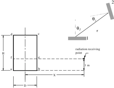
Equation A.1 assumes that the flame, under wind-free conditions, is a vertical cylinder with a diameter equal to that of the fire, and that the receiving element is a point located at a distance, X, from the base of the cylinder (Figure A.1).
H X 1 m a b c d e f D radiation receiving point r θ2 1 2 θ1
Figure A. 1 Quantities Used to Calculate View Factor
The integration is carried out over the entire surface of the flame. Assuming the point of interest to be a vertical receiving element (i.e., a person standing up), the vertical view factor for the case shown in Figure A.1 is [6]:
(
)
(
)
1/2 1 2 1 1/2 1/2 2 2 2 1 2 2 2 2 v 1 b 1 b tan b a 1 b a tan b 1 1 b 1 b 1) (b a 1) (b a tan 1) (b a 2 1) (b 2 a 1 b a b a F p 2 + − − − + + − − + + + × − + + + + + = − − − (A.2) Where: a = 2H(t) / D(t); and b = 2X / D(t).At locations very close to the fire, the maximum view factor is not very sensitive to the flame height. The observer at those locations already sees the maximum amount of flame surface and the increasing flame height does not affect the view factor significantly. On the other hand, at greater distance the view factors are very sensitive to the flame height.
To account for the fact that the target is located at a height of 1 m, rather than at the same height as the base of the fire, the cylinder used to represent the flame is divided into two parts: one above the height of the receiving point (fecd in Figure A.1) and one below the height of the receiving point (abef). The view factor from the entire flame is simply the sum of the view factors from each of the two cylinders to the receiving point.
APPENDIX B – HEAT TRANSFER TO BUILDING ELEMENTS
The FIERAsystem Building Element Failure Model (BEFM) [10] contains four sub-models that accommodate three types of materials: steel, concrete and wood. The BEFM calculates the time to failure of construction building elements, namely, steel columns and beams, concrete slabs and roofs, wooden beams, columns and assemblies, and thermal failure of wood stud assemblies. Some of these calculations are based on fire temperature histories provided by the Fire Development Model, which are then modified by the
Suppression Effectiveness Model to account for the effect of automatic suppression systems [12]. In the case of a ceiling, the ceiling impingement temperature is used to calculate the heat transfer to the compartment building. The equations used to calculate the ceiling impingement temperature are dependent on the heat release rate (e.g., see Equation 30). The FIERAsystem Suppression Effectiveness Model is able to take into account the effect of suppression systems on heat transfer to the ceiling by recalculating the ceiling impingement temperature using the modified heat release rate [12].
The walls of the compartment will be subjected to convective and radiative heat fluxes from both the flame and the plume gases. The FIERAsystem Building Element Failure Model [10] uses only a single temperature to represent the effects of the fire on the walls (e.g., the hot gas temperature in a fire resistant test furnace). Therefore, the
FIERAsystem Fire Development Model calculates an effective plume temperature (Tep) to
account for heat transfer from both the visible flame and the hot gases in the fire plume above the visible flame to the walls. This effective plume temperature is calculated based on a simple model of the thermal radiation heat transfer from the flame and hot gases. The view factors from the flame and hot gases are assumed to be proportional to their surface areas, and hence their heights. The initial wall temperature is assumed to be close to ambient. All emissivities are assumed to be one, and only thermal radiation heat transfer between the walls and the flame and hot gases are considered. The total thermal radiation heat flux from the flames and hot gases is then equated with the thermal radiation heat flux calculated using a single effective plume temperature:
(t) T H (t) H 1 (t) T H (t) H (t) T c4 c f 4 f c f 4 ep − + = (B.1) Where:
Hf(t) = the height of the flame (m); and
Hc = the height of the compartment (m).
Tc = ceiling impingement temperature
Tf = flame temperature
Tep = effective plume temperature
The effective plume temperature is output to the Suppression Effectiveness Model for each time step. The Suppression Effectiveness Model then modifies these temperatures at each time step based on the effect of suppression systems on the flame height, and then outputs the modified effective plume temperature to the Building Element Failure Model to determine the time to failure for each of the walls of the compartment.