HAL Id: hal-01275954
https://hal.inria.fr/hal-01275954
Submitted on 18 Feb 2016
HAL is a multi-disciplinary open access
archive for the deposit and dissemination of
sci-entific research documents, whether they are
pub-lished or not. The documents may come from
teaching and research institutions in France or
abroad, or from public or private research centers.
L’archive ouverte pluridisciplinaire HAL, est
destinée au dépôt et à la diffusion de documents
scientifiques de niveau recherche, publiés ou non,
émanant des établissements d’enseignement et de
recherche français ou étrangers, des laboratoires
publics ou privés.
Danai Symeonidou, Vincent Armant, Nathalie Pernelle, Fatiha Saïs
To cite this version:
Danai Symeonidou, Vincent Armant, Nathalie Pernelle, Fatiha Saïs. SAKey: Scalable Almost Key
Discovery in RDF Data. In proceedings of the 13th International Semantic Web Conference, ISWC
2014, Oct 2014, Riva del Garda, Italy. pp.33–49, �10.1007/978-3-319-11964-9_3�. �hal-01275954�
data
Danai Symeonidou1, Vincent Armant2, Nathalie Pernelle1, and Fatiha Saïs1
1 Laboratoire de Recherche en Informatique, University Paris Sud, France, 2 Insight Center for Data Analytics, University College Cork, Ireland
{danai.symeonidou,nathalie.pernelle,fatiha.sais}@lri.fr, {vincent.armant}@insight-centre.org
Abstract. Exploiting identity links among RDF resources allows appli-cations to efficiently integrate data. Keys can be very useful to discover these identity links. A set of properties is considered as a key when its values uniquely identify resources. However, these keys are usually not available. The approaches that attempt to automatically discover keys can easily be overwhelmed by the size of the data and require clean data. We present SAKey, an approach that discovers keys in RDF data in an efficient way. To prune the search space, SAKey exploits characteristics of the data that are dynamically detected during the process. Further-more, our approach can discover keys in datasets where erroneous data or duplicates exist (i.e., almost keys). The approach has been evaluated on different synthetic and real datasets. The results show both the relevance of almost keys and the efficiency of discovering them.
Keywords: Keys, Identity Links, Data Linking, RDF, OWL2
1
Introduction
Over the last years, the Web of Data has received a tremendous increase, con-taining a huge number of RDF triples. Integrating data described in different RDF datasets and creating semantic links among them, has become one of the most important goals of RDF applications. These links express semantic corre-spondences between ontology entities, or semantic links between data such as owl:sameAs links. By comparing the number of resources published on the Web with the number of owl:sameAs links, the observation is that the goal of building a Web of data is not accomplished yet.
Even if many approaches have been already proposed to automatically dis-cover owl:sameAs links (see [5] for a survey), only some are knowledge-based. In [16, 1], this knowledge can be expressive and specific linking rules can be learnt from samples of data. [13, 10] exploit key constraints, declared by a domain ex-pert, as knowledge for data linking. A key expresses a set of properties whose values uniquely identify every resource of a dataset. Keys can be used as logical rules to clean or link data when a high precision is needed, or to construct more
complex similarity functions [13, 7, 16]. Nevertheless, in most of the datasets pub-lished on the Web, the keys are not available and it can be difficult, even for an expert, to determine them.
Key discovery approaches have been proposed recently in the setting of the Semantic Web [3, 11]. [3] discovers pseudo keys, keys that do not follow the OWL2 semantics [12] of a key. This type of keys appears to be useful when a local completeness of data is known. [11] discovers OWL2 keys in clean data, when no errors or duplicates exist. However, this approach cannot handle the huge amount of data found on the Web.
Data published on the Web are usually created automatically, thus may con-tain erroneous information or duplicates. When these data are exploited to dis-cover keys, relevant keys can be lost. For example, let us consider a “dirty” dataset where two different people share the same social security number (SSN). In this case, SSN will not be considered as a key, since there exist two people sharing the same SSN. Allowing some exceptions can prevent the system from losing keys. Furthermore, the number of keys discovered in a dataset can be few. Even if a set of properties is not a key, it can lead to generate many correct links. For example, in most of the cases the telephone number of a restaurant is a key. Nevertheless, there can be two different restaurants located in the same place sharing phone numbers. In this case, even if this property is not a key, it can be useful in the linking process.
In this paper we present SAKey, an approach that exploits RDF datasets to discover almost keys that follow the OWL2 semantics. An almost key represents a set of properties that is not a key due to few exceptions (i.e., resources that do not respect the key constraint). The set of almost keys is derived from the set of non keys found in the data. SAKey can scale on large datasets by applying a number of filtering and pruning techniques that reduce the requirements of time and space. More precisely, our contributions are as follows:
1. the use of a heuristic to discover keys in erroneous data 2. an algorithm for the efficient discovery of non keys
3. an algorithm for the efficient derivation of almost keys from non keys The paper is organized as follows. Section 2 discusses the related works on key discovery and Section 3 presents the data and ontology model. Sections 4 and 5 are the main part of the paper, presenting almost keys and their discovery using SAKey. Section 6 presents our experiments before Section 7 concludes.
2
Related Work
The problem of discovering Functional Dependencies (FD) and keys has been intensively studied in the relational databases field. The key discovery problem can be viewed as a sub-problem of Functional Dependency discovery. Indeed, a FD states that the value of one attribute is uniquely determined by the val-ues of some other attributes. To capture the inherent uncertainty, due to data heterogeneity and data incompleteness, some approaches discover approximate keys and FDs instead of exact keys and FDs only. In [17], the authors propose
a way of retrieving non composite probabilistic FDs from a set of datasets. Two strategies are proposed: the first merges the data before discovering FDs, while the second merges the FDs obtained from each dataset. TANE [8] discovers ap-proximate FDs, i.e., FDs that almost hold. Each apap-proximate FD is associated to an error measure which is the minimal fraction of tuples to remove for the FD to hold in the dataset. For the key discovery problem, in relational context, Gor-dian method [14] allows discovering exact composite keys from relational data represented in a prefix-tree. To avoid scanning all the data, this method discov-ers first the maximal non keys and use them to derive the minimal keys. In [6], the authors propose DUCC, a hybrid approach for the discovery of minimal keys that exploits both the monotonic characteristic of keys and the anti-monotonic characteristic of non keys to prune the search space. To improve the efficiency of the approach, DUCC uses parallelization techniques to test different sets of attributes simultaneously.
In the setting of Semantic Web where data can be incomplete and may con-tain multivalued properties, KD2R [11] aims at deriving exact composite keys from a set of non keys discovered on RDF datasets. KD2R, extends [14] to be able to exploit ontologies and consider incomplete data and multivalued proper-ties. Nevertheless, even if KD2R [11] is able to discover composite OWL2 keys, it can be overwhelmed by large datasets and requires clean data. In [3], the au-thors have developed an approach based on TANE [8], to discover pseudo-keys (approximate keys) for which a set of few instances may have the same values for the properties of a key. The two approaches [11] and [3] differ on the seman-tics of the discovered keys in case of identity link computation. Indeed, the first considers the OWL2 [12] semantics, where in the case of multivalued properties, to infer an identity link between two instances, it suffices that these instances share at least one value for each property involved in the key, while in [3], the two instances have to share all the values for each property involved in the key, i.e., local completeness is assumed for all the properties (see [2] for a detailed comparison). In [15], to develop a data linking blocking method, discriminat-ing data type properties (i.e., approximate keys) are discovered from a dataset. These properties are chosen using unsupervised learning techniques and keys of specific size are explored only if there is no smaller key with a high discrimina-tive power. More precisely, the aim of [15] is to find the best approximate keys to construct blocks of instances and not to discover the complete set of valid minimal keys that can be used to link data.
Considering the efficiency aspect, different strategies and heuristics can be used to optimize either time complexity or space complexity. In both relational or Semantic Web settings, approaches can exploit monotonicity property of keys and the anti-monotonicity property of non keys to optimize the data exploration.
3
Data Model
RDF (Resource Description Framework) is a data model proposed by W3C used to describe statements about web resources. These statements are usually
rep-resented as triples <subject, property, object>. In this paper, we use a logical notation and represent a statement as property(subject, object).
An RDF dataset D can be associated to an ontology which represents the vocabulary that is used to describe the RDF resources. In our work, we consider RDF datasets that conform to OWL2 ontologies. The ontology O is presented as a tuple (C, P, A) where C is a set of classes3, P is a set of properties and A is a set of axioms.
In OWL24, it is possible to declare that a set of properties is a key for a
given class. More precisely, hasKey(CE(ope1, . . . , opem) (dpe1, . . . , dpen)) states
that each instance of the class expression CE is uniquely identified by the object
property expressions opei and the data property expressions dpej. This means
that there is no couple of distinct instances of CE that share values for all the object property expressions opeiand all the data type property expressions dpej
5 involved. The semantics of the construct owl:hasKey are defined in [12].
4
Preliminaries
4.1 Keys with Exceptions
RDF datasets may contain erroneous data and duplicates. Thus, discovering keys in RDF datasets without taking into account these data characteristics may lead to lose keys. Furthermore, there exist sets of properties that even if they are not keys, due to a small number of shared values, they can be useful for data linking or data cleaning. These sets of properties are particularly needed when a class has no keys.
In this paper, we define a new notion of keys with exceptions called n-almost keys. A set of properties is a n-almost key if there exist at most n instances that share values for this set of properties.
To illustrate our approach, we now introduce an example. Fig. 1 contains descriptions of films. Each film can be described by its name, the release date, the language in which it is filmed, the actors and the directors involved.
One can notice that the property d1:hasActor is not a key for the class F ilm since there exists at least one actor that plays in several films. Indeed, “G. Clooney” plays in films f 2, f 3 and f 4 while “M. Daemon” in f 1, f 2 and f 3. Thus, there exist in total four films sharing actors. Considering each film that shares actors with other films as an exception, there exist 4 exceptions for the property d1:hasActor. We consider the property d1:hasActor as a 4-almost key since it contains at most 4 exceptions.
Formally, the set of exceptions EP corresponds to the set of instances that
share values with at least one instance, for a given set of properties P .
3 c(i)will be used to denote that i is an instance of the class c where c ∈ C 4 http://www.w3.org/TR/owl2-overview
5 We consider only the class expressions that represent atomic OWL classes. An object
property expressionis either an object property or an inverse object property. The only allowed data type property expression is a data type property.
Dataset D1:
d1:Film(f1), d1:hasActor(f1,00B.P itt00), d1:hasActor(f1,00J.Roberts00),
d1:director(f1,00S.Soderbergh00), d1:releaseDate(f1,003/4/0100), d1:name(f1,00Ocean0s 1100),
d1:Film(f2), d1:hasActor(f2,00G.Clooney00), d1:hasActor(f2,00B.P itt00),
d1:hasActor(f2,00J.Roberts00), d1:director(f2,00S.Soderbergh00), d1:director(f2,00P.Greengrass00),
d1:director(f2,00R.Howard00), d1:releaseDate(f2,002/5/0400), d1:name(f2,00Ocean0s 1200)
d1:Film(f3), d1:hasActor(f3,00G.Clooney00), d1:hasActor(f3,00B.P itt00)
d1:director(f3,00S.Soderbergh00), d1:director(f3,00P.Greengrass00), d1:director(f3,00R.Howard00),
d1:releaseDate(f3,0030/6/0700), d1:name(f3,00Ocean0s 1300),
d1:Film(f4), d1:hasActor(f4,00G.Clooney00), d1:hasActor(f4,00N.Krause00),
d1:director(f4,00
A.P ayne00), d1:releaseDate(f4,00
15/9/1100), d1:name(f4,00 T he descendants00), d1:language(f4,00 english00) d1:Film(f5),d1:hasActor(f5,00 F.P otente00), d1:director(f5,00 P.Greengrass00), d1:releaseDate(f5,00200200), d1:name(f5,00
T he bourne Identity00), d1:language(f5,00
english00) d1:Film(f6),d1:director(f6,00 R.Howard00), d1:releaseDate(f6,00 2/5/0400), d1:name(f6,00 Ocean0s twelve00)
Fig. 1: Example of RDF data
Definition 1. (Exception set). Let c be a class (c ∈ C) and P be a set of
properties (P ⊆ P). The exception set EP is defined as:
EP = {X | ∃Y (X 6= Y ) ∧ c(X) ∧ c(Y ) ∧ (
^
p∈P
∃U p(X, U ) ∧ p(Y, U ))}
For example, in D1 of Fig. 1 we have: E{d1:hasActor} = {f 1, f 2, f 3, f 4},
E{d1:hasActor, d1:director}= {f 1, f 2, f 3}.
Using the exception set EP, we give the following definition of a n-almost key.
Definition 2. (n-almost key). Let c be a class (c ∈ C), P be a set of properties
(P ⊆ P) and n an integer. P is a n-almost key for c if |EP| ≤ n.
This means that a set of properties is considered as a n-almost key, if there exist from 1 to n exceptions in the dataset. For example, in D1 {d1:hasActor, d1:director} is a 3-almost key and also a n-almost key for each n ≥ 3. By definition, if a set of properties P is a n-almost key, every superset of P is also a almost key. We are interested in discovering only minimal n-almost keys, i.e., n-n-almost keys that do not contain subsets of properties that are n-almost keys for a fixed n.
4.2 Discovery of n-almost keys from n-non keys
To check if a set of properties is a n-almost key for a class c in a dataset D, a naive approach would scan all the instances of a class c to verify if at most n instances share values for these properties. Even when a class is described by few properties, the number of candidate n-almost keys can be huge. For example, if we consider a class c that is described by 60 properties and we aim to discover all the n-almost keys that are composed of at most 5 properties, the number of candidate n-almost keys that should be checked will be more than 6 millions. An efficient way to obtain n-almost keys, as already proposed in [14, 11], is to discover first all the sets of properties that are not n-almost keys and use them to derive the n-almost keys. Indeed, to show that a set of properties is not a
n-almost key, it is sufficient to find only (n+1) instances that share values for this set. We call the sets that are not n-almost keys, n-non keys.
Definition 3. (n-non key). Let c be a class (c ∈ C), P be a set of properties
(P ⊆ P) and n an integer. P is a n-non key for c if |EP| ≥ n.
For example, the set of properties {d1:hasActor, d1:director} is a 3-non key (i.e., there exist at least 3 films sharing actors and directors). Note that, every subset of P is also a n-non key since the dataset also contains n exceptions for this subset. We are interested in discovering only maximal n-non keys, i.e., n-non keys that are not subsets of other n-non keys for a fixed n.
5
The SAKey Approach
The SAKey approach is composed of three main steps: (1) the preprocessing steps that allow avoiding useless computations (2) the discovery of maximal (n+1)-non keys (see Algorithm 1) and finally (3) the derivation of n-almost keys from the set of(n+1)-non keys (see Algorithm 2).
5.1 Preprocessing Steps
Initially we represent the data in a structure called initial map. In this map, every set corresponds to a group of instances that share one value for a given property. Table 1 shows the initial map of the dataset D1 presented in Fig. 1. For example, the set {f 2, f 3, f 4} of d1:hasActor represents the films that “G.Clooney” has played in.
Table 1: Initial map of D1
d1:hasActor {{f1, f2, f3}, {f2, f3, f4}, {f1, f2}, {f4}, {f5}, {f6}} d1:director {{f1,f2,f3}, {f2, f3, f5}, {f2, f3, f6}, {f4}}
d1:releaseDate {{f1}, {f2, f6}, {f3}, {f4}, {f5}} d1:language {{f4, f5}}
d1:name {{f1}, {f2}, {f3}, {f4}, {f5}, {f6}}
Data Filtering. To improve the scalability of our approach, we introduce two techniques to filter the data of the initial map.
1. Singleton Sets Filtering. Sets of size 1 represent instances that do not share values with other instances for a given property. These sets cannot lead to the discovery of a n-non key, since n-non keys are based on instances that share values among them. Thus, only sets of instances with size bigger than 1 are kept. Such sets are called v-exception sets.
Definition 4. (v-exception set Epv). A set of instances {i1, . . . , ik} of the
class c is a Epv for the property p ∈ P and the value v iff {p(i1, v), . . . , p(ik, v)} ⊆
D and |{i1, . . . , ik}| > 1.
We denote by Ep the collection of all the v-exception sets of the property p.
For example, in D1, the set {f 1, f 2, f 3} is a v-exception set of the property d1:director.
Given a property p, if all the sets of p are of size 1 (i.e., Ep= ∅), this property
is a 1-almost key (key with no exceptions). Thus, singleton sets filtering allows the discovery of single keys (i.e., keys composed from only one property). In D1, we observe that the property d1:name is an 1-almost key.
2. v-exception Sets Filtering. Comparing the n-non keys that can be found by two v-exception sets Evi
p and E
vj
p , where Evpi⊆ E vj
p , we can ensure that the
set of n-non keys that can be found using Evi
p , can also be found using E
vj
p . To
compute all the maximal n-non keys of a dataset, only the maximal v-exception sets are necessary. Thus, all the non maximal v-exception sets are removed. For example, the v-exception set Ed1:hasActor“J. Roberts00 {f 1, f 2} in the property d1:hasActor represents the set of films in which the actress “J. Roberts” has played. Since there exists another actor having participated in more than these two films (i.e., “B, P itt” in films f 1, f 2 and f 3), the v-exception set {f 1, f 2} can be suppressed without affecting the discovery of n-non keys.
Table 2 presents the data after applying the two filtering techniques on the data of table 1. This structure is called final map.
Table 2: Final map of D1
d1:hasActor {{f1, f2, f3}, {f2, f3, f4}}
d1:director {{f1,f2,f3}, {f2, f3, f5}, {f2, f3, f6}} d1:releaseDate {{f2, f6}}
d1:language {{f4, f5}}
Elimination of Irrelevant Sets of Properties. When the properties are nu-merous, the number of candidate n-non keys is huge. However, in some cases, some combinations of properties are irrelevant. For example, in the DBpedia dataset, the properties depth and mountainRange are never used to describe the same instances of the class N aturalP lace. Indeed, depth is used to describe nat-ural places that are lakes while mountainRange natnat-ural places that are moun-tains. Therefore, depth and mountainRange cannot participate together in a n-non key. In general, if two properties have less than n instances in common, these two properties will never participate together to a n-non key. We denote by potential n-non key a set of properties sharing two by two, at least n instances. Definition 5. (Potential n-non key). A set of properties pnkn= {p1, ..., pm}
is a potential n-non key for a class c iff:
∀{pi, pj} ∈ (pnkn× pnkn) | I(pi) ∩ I(pj)| ≥ n
where I(p) is the set of instances that are subject of p.
To discover all the maximal n-non keys in a given dataset it suffices to find the n-non keys contained in the set of maximal potential n-non keys (P N K). For this purpose, we build a graph where each node represents a property and each edge between two nodes denotes the existence of at least n shared instances between these properties. The maximal potential n-non keys correspond to the
maximal cliques of this graph. The problem of finding all maximal cliques of a graph is NP-Complete [9]. Thus, we approximate the maximal cliques using a greedy algorithm inspired by the min-fill elimination order [4].
In D1, P N K = {{d1:hasActor, d1:director, d1:releaseDate},{d1:language}} corresponds to the set of maximal potential n-non keys when n=2. By con-struction, all the subsets of properties that are not included in these maximal potential n-non keys are not n-non keys.
5.2 n -non key Discovery
We first present the basic principles of the n-non key discovery. Then, we in-troduce the pruning techniques that are used by the nNonKeyFinder algorithm. Finally, we present the algorithm and give an illustrative example.
Basic Principles. Let us consider the property d1:hasActor. Since this prop-erty contains at least 3 exceptions, it is considered as a 3-non key. Intuitively, the set of properties {d1:hasActor, d1:director} is a 3-non key iff there exist at least 3 distinct films, such that each of them share the same actor and director with another film. In our framework, the sets of films sharing the same actor is represented by the collection of v-exception sets EhasActor, while the sets of
films sharing the same director is represented by the collection of v-exception sets Edirector. Intersecting each set of films of EhasActor with each set of films of
Edirector builds a new collection in which each set of films has the same actor
and the same director. More formally, we introduce the intersect operator ⊗ that intersects collections of exception sets only keeping sets greater than one. Definition 6. (Intersect operator ⊗). Given two collections of v-exception sets Ep and Ep0, we define the intersect ⊗ as follow:
Epi⊗ Epj = {E v pi∩ E v pj | E v pi∈ Epi, E v pj ∈ Epj, and |E v pi∩ E v pj| > 1}
Given a set properties P , the set of exceptions EP can be computed by applying
the intersect operator to all the collections Ep such that p ∈ P .
EP =
[ ⊗
p∈PEp
For example, for the set of properties P = {d1:hasActor, d1:hasDirector}, EP={{f1, f2, f3}, {f2, f3}} while EP = {f1, f2, f3}
Pruning Strategies. Computing the intersection of all the collections of v-exception sets represents the worst case scenario of finding maximal n-non keys within a potential n-non key. We have defined several strategies to avoid useless computations. We illustrate the pruning strategies in Fig. 2 where each level
corresponds to the collection Ep of a property p and the edges express the
in-tersections that should be computed in the worst case scenario. Thanks to the prunings, only the intersections appearing as highlighted edges are computed.
(a) Inclusion Pruning (b) Seen Intersection Pruning (c) example of nNonKeyFinder
Fig. 2: nNonKeyFinder prunings and execution
1. Antimonotonic Pruning. This strategy exploits the anti-monotonic char-acteristic of a n-non key, i.e., if a set of properties is a n-non key, all its subsets are by definition n-non keys. Thus, no subset of an already discovered n-non key will be explored.
2. Inclusion Pruning. In Fig. 2(a), the v-exception set of p1is included in one
of the v-exception sets of the property p2. This means that the biggest
intersec-tion between p1and p2is {i3, i4}. Thus, the other intersections of these two
prop-erties will not be computed and only the subpath starting from the v-exception set {i3, i4, i5} of p2 will be explored (bold edges in Fig. 2(a)). Given a set of
properties P = {p1, . . . , pj−1, pj, . . . , pn}, when the intersection of p1, . . . , pj−1
is included in any v-exception set of pj only this subpath is explored.
3. Seen Intersection Pruning. In Fig. 2(b), we observe that starting from the v-exception set of the property p1, the intersection between {i2, i3, i4} and
{i1, i2, i3} or {i2, i3, i5} will be in both cases {i2, i3}. Thus, the discovery using
the one or the other v-exception set of p2 will lead to the same n-almost keys.
More generally, when a new intersection is included in an already computed intersection, this exploration stops.
nNonkeyFinder Algorithm. To discover the maximal n-non keys, the v-exception sets of the final map are explored in a depth-first way. Since the
condition for a set of properties P to be a n-non key is EP ≥ n the exploration
stops as soon as n exceptions are found.
The algorithm takes as input a property pi, curInter the current intersection,
curN Key the set of already explored properties, seenInter the set of already computed intersections, nonKeySet the set of discovered n-non keys, E the set
of exceptions EP for each explored set of properties P , n the defined number of
exceptions and P N K the set of maximal potential n-non keys.
The first call of nNonKeyFinder is: nNonKeyFinder(pi, I, ∅, ∅, ∅, ∅, n, P N K)
where pi is the first property that belongs to at least one potential n-non key
and curInter the complete set of instances I. To ensure that a set of properties should be explored, the function uncheckedN onKeys returns the potential n-non keys that (1) contain this set of properties and (2) are not included in an already discovered n-non key in the nonKeySet. If the result is not empty, this set of properties is explored. In Line 3, the Inclusion pruning is applied i.e., if
the curInter is included in one of the v-exception sets of the property pi, the
selectedEp will contain only the curInter. Otherwise, all the v-exception sets of
all the maximal n-non keys using this v-exception set are discovered. To do so, the current intersection (curInter) is intersected with the selected v-exception sets of the property pi. If the new intersection (newInter) is bigger than 1 and
has not been seen before (Seen intersection pruning), then pi∪ curN onKey is
stored in nvN key. The instances of newInter are added in E for nvN key using the update function. If the number of exceptions for a given set of properties is bigger than n, then this set is added to the nonKeySet. The algorithm is called
with the next property pi+1 (Line 16). When the exploration of an intersection
(newInter) is done, this intersection is added to SeenInter. Once, all the
n-non keys for the property pi have been found, nNonKeyFinder is called for the
property pi+1 with curInter and curN Key (Line 19), forgetting the property
pi in order to explore all the possible combinations of properties.
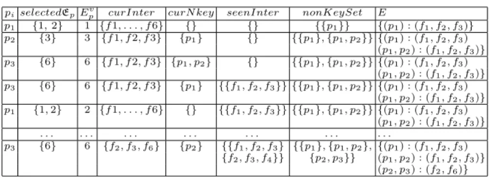
Table 3 shows the execution of nNonKeyFinder for the example presented in Fig. 2(c) where P N K = {{d1:hasActor, d1:director, d1:releaseDate}}. We represent the properties in Table 3 by p1, p2, p3respectively.
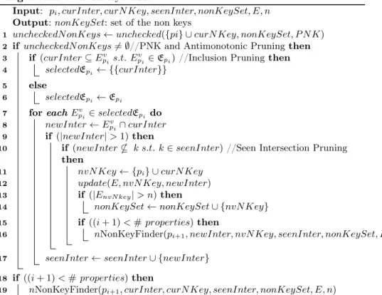
Algorithm 1: nNonKeyFinder
Input: pi, curInter, curN Key, seenInter, nonKeySet, E, n
Output: nonKeySet: set of the non keys
1 uncheckedN onKeys ← unchecked({pi} ∪ curN Key, nonKeySet, P N K) 2 if uncheckedN onKeys 6= ∅//PNK and Antimonotonic Pruning then 3 if (curInter ⊆ Ev
pis.t. E v
pi∈ Epi)//Inclusion Pruning then
4 selectedEpi ← {{curInter}}
5 else
6 selectedEpi ← Epi
7 for each Epvi∈ selectedEpi do
8 newInter ← Epvi∩ curInter
9 if (|newInter| > 1) then
10 if (newInter * k s.t. k ∈ seenInter) //Seen Intersection Pruning then
11 nvN Key ← {pi} ∪ curN Key
12 update(E, nvN Key, newInter) 13 if (|EnvN key| > n) then
14 nonKeySet ← nonKeySet ∪ {nvN Key} 15 if ((i + 1) < # properties) then
16 nNonKeyFinder(pi+1, newInter, nvN Key, seenInter, nonKeySet, E, n)
17 seenInter ← seenInter ∪ {newInter} 18 if ((i + 1) < # properties) then
Table 3: nNonKeyFinder execution on the example of Fig. 2(c)
piselectedEpEpv curInter curN key seenInter nonKeySet E
p1 {1, 2} 1 {f 1, . . . , f 6} {} {} {{p1}} {(p1) : (f1, f2, f3)} p2 {3} 3 {f 1, f 2, f 3} {p1} {} {{p1}, {p1, p2}}{(p1) : (f1, f2, f3) (p1, p2) : (f1, f2, f3)} p3 {6} 6 {f 1, f 2, f 3} {p1, p2} {} {{p1}, {p1, p2}}{(p1) : (f1, f2, f3) (p1, p2) : (f1, f2, f3)} p3 {6} 6 {f 1, f 2, f 3} {p1} {{f1, f2, f3}} {{p1}, {p1, p2}}{(p1) : (f1, f2, f3) (p1, p2) : (f1, f2, f3)} p1 {1, 2} 2 {f 1, . . . , f 6} {} {{f1, f2, f3}} {{p1}, {p1, p2}}{(p1) : (f1, f2, f3) (p1, p2) : (f1, f2, f3)} . . . . p3 {6} 6 {f2, f3, f6} {p2} {{f1, f2, f3} {{p1}, {p1, p2},{(p1) : (f1, f2, f3) {f2, f3, f4}} {p2, p3}} (p1, p2) : (f1, f2, f3)} (p2, p3) : (f2, f6)} 5.3 Key Derivation
In this section we introduce the computation of minimal n-almost keys using maximal (n+1)-non keys. A set of properties is a n-almost key, if it is not equal or included to any maximal (n+1)-non key. Indeed, when all the (n+1)-non keys are discovered, all the sets not found as (n+1)-non keys will have at most n exceptions (n-almost keys).
Both [14] and [11] derive the set of keys by iterating two steps: (1) com-puting the Cartesian product of complement sets of the discovered non keys and (2) selecting only the minimal sets. Deriving keys using this algorithm is very time consuming when the number of properties is big. To avoid useless computations, we propose a new algorithm that derives fast minimal n-almost keys, called keyDerivation. In this algorithm, the properties are ordered by their frequencies in the complement sets. At each iteration, the most frequent prop-erty is selected and all the n-almost keys involving this propprop-erty are discovered recursively. For each selected property p, we combine p with the properties of the selected complement sets that do not contain p. Indeed, only complement sets that do not contain this property can lead to the construction of minimal n-almost keys. When all the n-almost keys containing p are discovered, this prop-erty is eliminated from every complement set. When at least one complement set is empty, all the n-almost keys have been discovered. If every property has a different frequency in the complement sets, all the n-almost keys found are min-imal n-almost keys. In the case where two properties have the same frequency, additional heuristics should be taken into account to avoid computations of non minimal n-almost keys.
Let us illustrate the key derivation algorithm throughout and
example. Let P= {p1, p2, p3, p4, p5} be the set of properties and
{{p1, p2, p3}, {p1, p2, p4}, {p2, p5}, {p3, p5}} the set of maximal n-non
keys. In this example, the complement sets of n-non keys are {{p1, p2, p4},
{p1, p3, p4}, {p3, p5},{p4, p5}}. The properties of this example are explored
in the following order: {p4, p1, p3, p5, p2}. Starting from the most frequent
selected complement set that does not contain this property is {p3, p5}. The
property p4 is combined with every property of this set. The set of n-almost
keys is now {{p3, p4}, {p4, p5}}. The next property to be explored is p1. The
selected complement sets are {p5} and {p3, p5}. To avoid the discovery of
non-minimal n-almost keys, we order the properties of the selected complement sets, according to their frequency (i.e., {p5, p3}). To discover n-almost keys
containing p1 and p5, we only consider the selected complement sets that do
not contain p5. In this case, no complement set is selected and the key {p1, p5}
is added to the n-almost keys. p5 is locally suppressed for p1. Since there is an
empty complement set, all the n-almost keys containing p1 are found and p1 is
removed from the complement sets. Following these steps, the set of minimal n-almost keys in the end will be {{p1, p5}, {p2, p3, p5}, {p3, p4}, {p4, p5}}.
Algorithm 2: keyDerivation
Input: compSets: set of complement sets Output: KeySet: set of n-almost keys 1 KeySet ← ∅
2 orderedP roperties= getOrderedProperties(compSets) 3 for each pi∈ orderedP roperties do
4 selectedCompSets ←selectSets(pi, compSets)
5 if (selectedCompSets == ∅) then 6 KeySet = KeySet ∪ {{pi}}
7 else
8 KeySet = KeySet ∪ {pi×keyDerivation(selectedCompSets)}
9 compSets= remove(compSets, pi)
10 if ( ∃ set ∈ compSet s.t. set == ∅ ) then 11 break
12 return KeySet
6
Experiments
We evaluated SAKey using 3 groups of experiments. In the first group, we demon-strate the scalability of SAKey thanks to its filtering and pruning techniques. In the second group we compare SAKey with KD2R, the only approach that dis-covers composite OWL2 keys. The two approaches are compared in two steps. First, we compare the runtimes of their non key discovery algorithms and second, the runtimes of their key derivation algorithms. Finally, we show how n-almost keys can improve the quality of data linking. The experiments are executed on
3 different datasets, DBpedia6, YAGO7 and OAEI 20138.
The execution time of each experiment corresponds to the average time of 10 repetitions. In all experiments, the data are stored in a dictionary-encoded map,
6 http://wiki.dbpedia.org/Downloads39
7 http://www.mpi-inf.mpg.de/yago-naga/yago/downloads.html 8 http://oaei.ontologymatching.org/2013
where each distinct string appearing in a triple is represented by an integer. The experiments have been executed on a single machine with 12GB RAM, processor 2x2.4Ghz, 6-Core Intel Xeon and runs Mac OS X 10.8.
6.1 Scalability of SAKey
SAKey has been executed in every class of DBpedia. Here, we present the scalability on the classes DB:N aturalP lace, DB:BodyOf W ater and DB:Lake of DBpedia (see Fig. 3(b) for more details) when n = 1. We first compare the size of data before and after the filtering steps (see Table 4), and then we run SAKey on the filtered data with and without applying the prunings (see Table 5). Data Filtering Experiment. As shown in Table 4, thanks to the filtering steps, the complete set of n-non keys can be discovered using only a part of the data. We observe that in all the three datasets more than 88% of the sets of instances of the initial map are filtered applying both the singleton filtering and the v-exception set filtering. Note that more than 50% of the properties are suppressed since they are single 1-almost keys (singleton filtering).
Table 4: Data filtering results on different DBpedia classes
class # Initial sets # Final sets # Singleton sets # Ev
pfiltered Suppressed Prop.
DB:Lake 57964 4856(8.3%) 50807 2301 78 (54%) DB:BodyOfW ater 139944 14833(10.5%) 120949 4162 120 (60%)
DB:NaturalP lace 206323 22584(11%) 177278 6461 131 (60%)
Prunings of SAKey. To validate the importance of our pruning techniques, we run nNonKeyFinder on different datasets with and without prunings. In Table 5, we show that the number of calls of nNonKeyFinder decreases significantly using the prunings. Indeed, in the class DB:Lake the number of calls decreases to half. Subsequently, the runtime of SAKey is significantly improved. For example, in the class DB:N aturalP lace the time decreases by 23%.
Table 5: Pruning results of SAKey on different DBpedia classes
class without prunings with prunings Calls Runtime Calls Runtime DB:Lake 52337 13s 25289 (48%) 9s DB:BodyOfW ater 443263 4min28s 153348 (34%) 40s
DB:NaturalP lace 1286558 5min29s 257056 (20%) 1min15s
To evaluate the scalability of SAKey when n increases, nNonKeyFinder has been executed with different n values. This experiment has shown that nNonKeyFinder is not strongly affected by the increase of n. Indeed, allow-ing 300 exceptions (n=300) for the class DB:N aturalP lace, the execution time increases only by 2 seconds.
6.2 KD2R vs. SAKey: Scalability Results
In this section, we compare SAKey with KD2R in two steps. The first experi-ment compares the efficiency of SAKey against KD2R in the non key discovery
1
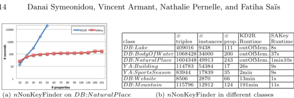
# # # KD2R SAKey class triples instances prop. Runtime Runtime DB:Lake 409016 9438 111 outOfMem. 8s DB:BodyOfW ater 1068428 34000 200 outOfMem. 37s DB:NaturalP lace 1604348 49913 243 outOfMem. 1min10s Y A:Building 114783 54384 17 26s 9s Y A:SportsSeason 83944 17839 35 2min 9s DB:W ebsite 8506 2870 66 13min 1s DB:Mountain 115796 12912 124 191min 11s
(a) nNonKeyFinder on DB:NaturalP lace (b) nNonKeyFinder in different classes
Fig. 3: nNonKeyFinder runtime for DBpedia and YAGO classes
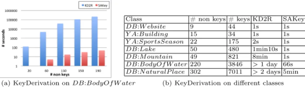
process. Given the same set of non keys, the second experiment compares the key discovery approach of KD2R against the one of SAKey. Note that, to obtain the same results from both KD2R and SAKey, the value of n is set to 1. n-non key Discovery. In Fig. 3(a), we compare the runtimes of the non key discovery of both KD2R and SAKey for the class DB:N aturalP lace. Starting from the 10 most frequent properties, properties are added until the whole set of properties is explored. We observe that KD2R is not resistant to the number of properties and its runtime increases exponentially. For example, when the 50 most frequent properties are selected, KD2R takes more than five hours to discover the non keys while SAKey takes only two minutes. Moreover, we notice that SAKey is linear in the beginning and almost constant after a certain size of properties. This happens since the class DB:N aturalP lace contains many single keys and unlike KD2R, SAKey is able to discover them directly using the singleton sets pruning. In Fig. 3(b), we observe that SAKey is orders of magnitude faster than KD2R in classes of DBpedia and YAGO. Moreover, KD2R runs out of memory in classes containing many properties and triples. n-almost key Derivation. We compare the runtimes of the key derivation of KD2R and SAKey on several sets of non keys. In Fig. 4(a), we present how the time evolves when the number of non keys of the class DB:BodyOf W ater increases. SAKey scales almost linearly to the number of non keys while the time of KD2R increases significantly. For example, when the number of non keys is 180, KD2R needs more than 1 day to compute the set of minimal keys while SAKey less than 1 minute. Additionally, to show the efficiency of SAKey over KD2R, we compare their runtimes on several datasets (see Fig. 4(b)). In every case, SAKey outperforms KD2R since it discovers fast the set of minimal keys.
In the biggest class of DBpedia, DB:P erson (more than 8 million triples, 9 hundred thousand instances and 508 properties), SAKey takes 19 hours to compute the n-non keys while KD2R cannot even be applied.
6.3 Data Linking with n-almost keys
Here, we evaluate the quality of identity links that can be found using n-almost keys. We have exploited one of the datasets provided by the OAEI’13. The benchmark contains one original file and five test cases. The second file is taken
1 Class # non keys # keys KD2R SAKey
DB:W ebsite 9 44 1s 1s Y A:Building 15 34 1s 1s Y A:SportsSeason 22 175 2s 1s DB:Lake 50 480 1min10s 1s DB:Mountain 49 821 8min 1s DB:BodyOfW ater 220 3846 >1 day 66s DB:NaturalP lace 302 7011 >2 days 5min (a) KeyDerivation on DB:BodyOfW ater (b) KeyDerivation on different classes
Fig. 4: KeyDerivation runtime for DBpedia and YAGO classes
from the first test case. Both files contain DBpedia descriptions of persons and locations (1744 triples, 430 instances, 11 properties). Table 6 shows the results when n varies from 0 to 18. In Table 6(a), strict equality is used to compare literal values while in Table 6(b), the Jaro-Winkler similarity measure is used. The recall, precision and F-measure of our linking results has been computed using the gold-standard provided by OAEI’13.
Table 6: Data Linking in OAEI 2013
# exceptions Recall Precision F-Measure 0, 1, 2 25.6% 100% 41%
3, 4 47.6% 98.1% 64.2% 5, 6 47.9% 96.3% 63.9% 7, ..., 17 48.1% 96.3% 64.1% 18 49.3% 82.8% 61.8%
# exceptions Recall Precision F-Measure 0, 1, 2 64.4% 92.3% 75.8%
3, 4 73.7% 90.8% 81.3% 5, 6 73.7% 90.8% 81.3% 7, ..., 17 73.7% 90.8% 81.3% 18 74.4% 82.4% 78.2% (a) Data Linking using strict equality (b) Data Linking using similarity measures
In both tables, we observe that the quality of the data linking improves when few exceptions are allowed. As expected, when simple similarity measures are used, the recall increases while the precision decreases, but overall, better F-measure results are obtained. As shown in [11],using keys to construct complex similarity functions to link data, such as [13], can increase even more the recall. Therefore, linking results can be improved when n-almost keys are exploited by sophisticated data linking tools.
7
Conclusion
In this paper, we present SAKey, an approach for discovering keys on large RDF data under the presence of errors and duplicates. To avoid losing keys when data are “dirty”, we discover n-almost keys, keys that are almost valid in a dataset. Our system is able to scale when data are large, in contrast to the state-of the art that discovers composite OWL2 keys. Our extensive experiments show that SAKey can run on millions of triples. The scalability of the approach is validated on different datasets. Moreover, the experiments demonstrate the relevance of the discovered keys.
In our future work, we plan to define a way to automatically set the value of n, in order to ensure the quality of a n-almost key. Allowing no exceptions might be very strict in RDF data while allowing a huge number of exceptions
might end up to many false negatives. We also aim to define a new type of keys, the conditional keys which are keys valid in a subset of the data.
SAKey is available for download at https://www.lri.fr/sakey. Acknowledgments
This work is supported by the ANR project Qualinca (QUALINCA-ANR-2012-CORD-012-02).
References
1. Arasu, A., Ré, C., Suciu, D.: Large-scale deduplication with constraints using dedu-palog. In: ICDE. pp. 952–963 (2009)
2. Atencia, M., Chein, M., Croitoru, M., Jerome David, M.L., Pernelle, N., Saïs, F., Scharffe, F., Symeonidou, D.: Defining key semantics for the rdf datasets: Experi-ments and evaluations. In: ICCS (2014)
3. Atencia, M., David, J., Scharffe, F.: Keys and pseudo-keys detection for web datasets cleansing and interlinking. In: EKAW. pp. 144–153 (2012)
4. Dechter, R.: Constraint Processing. Morgan Kaufmann Publishers Inc., San Fran-cisco, CA, USA (2003)
5. Ferrara, A., Nikolov, A., Scharffe, F.: Data linking for the semantic web. Int. J. Semantic Web Inf. Syst. 7(3), 46–76 (2011)
6. Heise, A., Jorge-Arnulfo, Quiane-Ruiz, Abedjan, Z., Jentzsch, A., Naumann, F.: Scalable discovery of unique column combinations. VLDB 7(4), 301–312 (2013) 7. Hu, W., Chen, J., Qu, Y.: A self-training approach for resolving object coreference
on the semantic web. In: WWW. pp. 87–96 (2011)
8. Huhtala, Y., Kärkkäinen, J., Porkka, P., Toivonen, H.: Tane: An efficient algorithm for discovering functional and approximate dependencies. The Computer Journal 42(2), 100–111 (1999)
9. Karp, R.M.: Reducibility among combinatorial problems. In: Miller, R.E., Thatcher, J.W. (eds.) Complexity of Computer Computations. pp. 85–103. The IBM Research Symposia Series (1972)
10. Nikolov, A., Motta, E.: Data linking: Capturing and utilising implicit schema-level relations. In: Proceedings of Linked Data on the Web workshop at WWW (2010) 11. Pernelle, N., Saïs, F., Symeonidou, D.: An automatic key discovery approach for
data linking. J. Web Sem. 23, 16–30 (2013)
12. Recommendation, W.: Owl2 web ontology language: Direct semantics. In: Motik B., Patel-Schneider P. F., C.G.B. (ed.) http://www.w3.org/TR/owl2-direct-semantics. W3C (27 October 2009)
13. Saïs, F., Pernelle, N., Rousset, M.C.: Combining a logical and a numerical method for data reconciliation. Journal on Data Semantics 12, 66–94 (2009)
14. Sismanis, Y., Brown, P., Haas, P.J., Reinwald, B.: Gordian: efficient and scalable discovery of composite keys. In: VLDB. pp. 691–702 (2006)
15. Song, D., Heflin, J.: Automatically generating data linkages using a domain-independent candidate selection approach. In: ISWC. pp. 649–664 (2011)
16. Volz, J., Bizer, C., Gaedke, M., Kobilarov, G.: Discovering and maintaining links on the web of data. In: ISWC. pp. 650–665 (2009)
17. Wang, D.Z., Dong, X.L., Sarma, A.D., Franklin, M.J., Halevy, A.Y.: Functional dependency generation and applications in pay-as-you-go data integration systems. In: WebDB (2009)