Publisher’s version / Version de l'éditeur: Building Acoustics, 6, September, pp. 289-308, 1999
READ THESE TERMS AND CONDITIONS CAREFULLY BEFORE USING THIS WEBSITE. https://nrc-publications.canada.ca/eng/copyright
Vous avez des questions? Nous pouvons vous aider. Pour communiquer directement avec un auteur, consultez la
première page de la revue dans laquelle son article a été publié afin de trouver ses coordonnées. Si vous n’arrivez pas à les repérer, communiquez avec nous à PublicationsArchive-ArchivesPublications@nrc-cnrc.gc.ca.
Questions? Contact the NRC Publications Archive team at
PublicationsArchive-ArchivesPublications@nrc-cnrc.gc.ca. If you wish to email the authors directly, please see the first page of the publication for their contact information.
This publication could be one of several versions: author’s original, accepted manuscript or the publisher’s version. / La version de cette publication peut être l’une des suivantes : la version prépublication de l’auteur, la version acceptée du manuscrit ou la version de l’éditeur.
For the publisher’s version, please access the DOI link below./ Pour consulter la version de l’éditeur, utilisez le lien DOI ci-dessous.
https://doi.org/10.1260/1351010991501356
Access and use of this website and the material on it are subject to the Terms and Conditions set forth at
Structure-borne sound transmission in rib-stiffened plate structures typical of wood frame buildings
Bosmans, I.; Nightingale, T. R. T.
https://publications-cnrc.canada.ca/fra/droits
L’accès à ce site Web et l’utilisation de son contenu sont assujettis aux conditions présentées dans le site
LISEZ CES CONDITIONS ATTENTIVEMENT AVANT D’UTILISER CE SITE WEB.
NRC Publications Record / Notice d'Archives des publications de CNRC:
https://nrc-publications.canada.ca/eng/view/object/?id=42e84300-e010-4021-911e-7422cb6fca0c https://publications-cnrc.canada.ca/fra/voir/objet/?id=42e84300-e010-4021-911e-7422cb6fca0c
Bosmans, I.; Nightinghale, T. R. T.
A version of this paper is published in / Une version de ce document se trouve dans : Building Acoustics, v. 6, no. 3/4, 1999, p. 289-308
www.nrc.ca/irc/ircpubs
Structure-Borne Sound Transmission in Rib-stiffened Plate Structures Typical Of
Wood Frame Buildings.
Ivan Bosmans and Trevor R.T. Nightingale
National Research Council Canada, Institute for Research in Construction, Acoustics, Montreal Road, Ottawa, Ontario, K1A 0R6, Canada.
SUMMARY
Structure-borne sound transmission at a subfloor/joist connection typical of wood frame buildings is investigated experimentally and theoretically. The first part of this paper investigates the influence of the fastener spacing on the vibration attenuation across a joist. For this purpose, measurements were carried out on a small floor section for various coupling conditions of the joist. The experimental results suggested the existence of an effective coupling area characterizing the screwed joist/floor connection. In the second part of this study, a calculation model is developed based on Statistical Energy Analysis (SEA) and plate strip theory for the idealized case of a rigid line connection. The presented model is verified experimentally on a Plexiglas structure and a subfloor/joist connection. The experimental validation showed fair agreement between measured and calculated data, but revealed that more work is required to improve the prediction accuracy in realistic situations.
1. INTRODUCTION
Over the past few decades, calculation models predicting structure-borne sound transmission in buildings have almost exclusively been developed by European scientists [1-8]. As a result, these prediction models were originally intended for masonry and concrete buildings, which represent the most common construction type for residential buildings in Europe. In contrast, modeling flanking transmission in lightweight structures remains a relatively new research topic. A recent contribution to this field was reported by Craik et al. [9], who investigated the airborne sound transmission through a double leaf partition in the presence of a fire stop. The effect of flanking transmission through the fire stop was estimated based on a simplified bending wave model. Part of the apparent lack of other theoretical research can be explained by the complexity of wood frame constructions. Only recent developments in analytical modeling have provided the necessary tools for assessing the influence of the anisotropic nature of the materials [10] and the ‘point’ connections using screws or nails [11].
As demonstrated by the work of Craik et al. [9], the dominant flanking path in wood frame buildings often involves the floor/ceiling assembly. Figure 1 illustrates that a typical wood frame floor consists of a subfloor of Oriented Strand Board (OSB) or plywood which is supported by a series of parallel wood joists. The subfloor is connected to the joists by a number of equally spaced screws. If the influence of the suspended ceiling and the cross-bridging is ignored in a first approximation, the floor is essentially a rib-stiffened plate structure. As a result, modeling structure-borne sound transmission in a floor requires an accurate understanding of the subfloor/joist interaction. In this paper, a subfloor/joist connection typical of floors in wood frame buildings is investigated experimentally and theoretically. The aim of this study is to identify the various parameters (e.g. joist depth, fastener spacing and material properties) which need to be considered when modeling flanking transmission through a wood frame floor.
In the first part of this paper, the frequency dependent behavior of the joist/floor connection is investigated based on a series of measurements corresponding to different coupling conditions of the joist. Next, a theoretical calculation model using SEA will be presented for the ideal case of a line connection. This calculation model will be verified experimentally on a homogeneous and isotropic structure as well as on a realistic joint. Distinction will be made between three different approaches, each characterized by a proper procedure for modeling the joist. The analysis will focus only on structure-borne sound transmission in a direction normal to the joist. Although reference will be made only to floors, the connections between gypsum board walls and the supporting framing members are very similar to subfloor/joist connections. Consequently, the theoretical and experimental results presented in this paper are equally relevant to structure-borne sound transmission in lightweight walls.
2. CHARACTERIZING THE SUBFLOOR/JOIST CONNECTION
Characterizing structural connections that use nails or screws represents a major difficulty of modeling flanking transmission in wood frame buildings. In the context of lightweight walls, it has been suggested that the joint between a gypsum board sheet and a wood stud should be treated as a line connection at low frequencies and a series of point connections at high frequencies [12]. The transition between both regimes was found to be the frequency at which the spacing between the nails matched half the bending wavelength in the gypsum board. This simplified approach assumes an infinitely small contact area between the plate and the beam element. In addition, it treats the plate as one entire
subsystem and therefore neglects the vibration attenuation across the framing member. The experimental data presented in the following paragraphs will show that these assumptions are inappropriate for the junction under consideration in this paper.
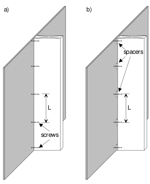
The influence of the screw spacing on structure-borne sound transmission at a subfloor/joist connection is investigated by two series of measurements in laboratory conditions. One OSB sheet (2.4 x 1.2 x 0.0147 m) was connected to a wood joist (1.2 x 0.235 x 0.037 m) using nominally equally spaced screws. The joist divided the OSB sheets into two nominally identical plates measuring 1.2 x 1.2 m. Figure 2 shows that the assembly was mounted on a resilient layer in order to obtain adequate decoupling from the laboratory floor. Two strings were attached to the corners of the OSB sheet to keep the specimen in the vertical position. In the first series, the OSB sheet was attached to the joist by 5, 9 and 17 equally spaced screws, corresponding to a screw spacing, L, of 0.3, 0.15 and 0.075 m (Figure 3a). In the second series of tests, the same number of screws was considered, but a thin aluminum plate (0.038 x 0.038 x 0.001 m) was positioned between the joist and the OSB sheet at each of the fasteners (Figure 3b). The aluminum spacers were applied to create a well defined contact area at the joint. It should be noted that the thin layer of air between the joist and the OSB sheet might lead to an increase of the damping due to air pumping effects. In view of the relatively high internal loss of the building materials in wood frame buildings, it is assumed that the additional damping is negligible.
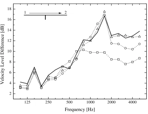
The velocity level difference measurements were carried out using a two channel technique as reported by Craik [13]. Using this method, the transverse velocity level is measured in one randomly positioned measurement point on each plate while the source plate is excited using uniformly distributed hammer blows. The average velocity level difference between the source and the receiving plate is estimated by repeating this procedure for several pairs of measurement points until the average converges to a stable value. The one-third-octave band results of the two series are shown in Figures 4 and 5. All results were compared to a line junction, which corresponds to a combination of glue and 17 screws.
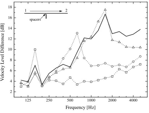
Figure 4 shows that the 17 screw connection behaves as a line junction over the entire frequency range. The case with 9 fasteners approximates a line connection up to 2 kHz, whereas the case with 5 screws does the same up to 800 Hz. Above these cut-off frequencies, the velocity level difference drops, indicating a weakened coupling between the joist and the plate. By comparing Figures 4 and 5, it can be observed that the connections with spacers are characterized by considerably lower cut-off
frequencies. This leads to the conclusion that the transition from line to ‘local’ connection is not determined exclusively by the spacing between the fasteners. Moreover, the results indicate that a realistic subfloor/joist connection is characterized by an effective contact area which is considerably greater than the cross-section area of the fastener. These conclusions demonstrate the necessity for a more sophisticated approach which does not make any simplifying assumptions concerning the transition from line to ‘local’ connection and which allows a finite contact area at the joint. The model developed by Bosmans and Vermeir [11] satisfies these requirements, but needs modifications to more accurately represent the junction under investigation.
3. MODELLING THE JOISTS
In SEA, beams at plate/beam junctions are often considered as undamped coupling elements and not as subsystems [8,14]. The influence of a beam is taken into account when calculating the coupling loss factor, since the presence of the beam changes the impedance of the junction and therefore also the energy flow between the coupled plates. As cross-section deformation is typically not included, this approach is particularly suited for beams having a rectangular cross-section and an aspect ratio close to unity. However, since the aspect ratio of a joist cross-section is usually larger than 6, some deformation is likely to occur at relatively low frequencies. As a result, the impedance at the junction is considerably overestimated when the cross-section is modeled as infinitely rigid. In fact, it is more appropriate to model the joist as an undamped plate strip [12,15]. Also in this case, the joist is not included as a subsystem in the SEA model. Figure 6 illustrates that a plate strip model allows the joist to bend in the plane of its cross-section, whereas, in the eccentric beam model, the cross-section behaves as a rigid body.
Modeling the joist as an undamped plate strip is justified as long as the energy dissipation in the joist is negligible compared to the damping of the OSB plates. This implies that the plate strip model should be applied in a frequency range where the joists support only few modes. At high frequencies, the dissipation cannot be ignored and the joists should be modeled as plate subsystems in order to obtain the correct energy distribution in the floor. In this case, coupling loss factors should be calculated by modeling the subfloor/joist junction as a T-joint.
As a first step towards modeling structure-borne sound transmission through floors, a model is presented for the idealized case of a rigid line connection. The model is based on a wave formulation
for junctions of semi-infinite, orthotropic plates. The theory allows a joist to be modeled as an eccentric Timoshenko beam, a plate strip or a semi-infinite plate
3.1 Wave approach for orthotropic plates
Coupling loss factors describing the energy flow between two plate subsystems in an SEA model are often calculated based on the so-called wave approach. In this method, vibrational energy flow between plates is assessed by modeling reflection and transmission of structure-borne sound waves at junctions of semi-infinite plates coupled along a common edge. The excitation of the plate assembly is taken as a plane wave incident upon the junction on one of the plates. The incident wave generates bending and in-plane waves propagating away from the junction on all plates, where the propagation direction of the waves is determined by Snell's law. The forces and displacements at the plate edges are expressed in terms of the amplitudes of these propagating waves. The equilibrium and continuity conditions at the junction line lead to a set of linear equations, the solution of which yields the unknown wave amplitudes. The energy flow associated with each traveling wave is determined by its amplitude. Structure-borne sound transmission is quantified by the transmission coefficient, which is defined as the ratio of the transmitted intensity to the intensity carried by the incident wave. Based on the assumption of a diffuse wavefield on the source plate, the transmission coefficient is averaged over all angles of incidence. Finally, the angle-averaged result is used to calculate the SEA coupling loss factor. Wöhle et al. [2,3] and Craven et al. [4,5] have developed the wave approach for the basic case of a rigid junction between thin isotropic plates. However, the materials used in wood frame buildings are strongly orthotropic. The wood chips in OSB are predominantly oriented parallel to the long axis of the sheet. As a result, the bending stiffness in this direction is approximately 2-4 times higher than in the direction of the short axis. The anisotropy in dimensional lumber is even more pronounced, since the ratio of the Young’s modulus in the grain direction to the Young’s modulus normal the grain can be as high as 30. In order to take into account the orthotropic behavior of these materials, a model was developed for junctions of thin orthotropic plates.
Analytical solutions to the equations of motion for bending and in-plane waves for thin orthotropic plates have been derived by Bosmans et al. [10,16]. Two typical features of wave propagation in orthotropic plates are that the structural intensity is not parallel to the propagation direction of a plane wave and the vibrational energy is not distributed uniformly over all directions in a reverberant field.
These properties have important implications for the application in an SEA model, since they require a new derivation of the coupling loss factor. Further, in-plane wave propagation cannot be separated into pure quasi-longitudinal and shear waves, but rather into a fast and a slow in-plane wave. However, both wave types are characterized by a mixture of quasi-longitudinal and shear wave motion.
In this paper, the theory presented in [10] and [16] is modified in order to include an orthotropic stiffening rib at the joint. The stiffening rib is modeled either as an orthotropic plate strip, or as an eccentric beam. For this purpose, the orthotropic plate model is modified using concepts of plate strip theory [12,15] and plate/beam joint modeling [8,14]. The following paragraphs will focus mostly on the description of the stiffening rib, since other aspects are sufficiently dealt with in literature.
3.2 Plate strip model.
The geometry of a rigid plate strip joint is shown in Figure 7. The junction consists of an assembly of semi-infinite plates and plate strips coupled by a junction beam. The junction beam is introduced as an artificial coupling element which facilitates the description of the boundary conditions at the joint. When modeling a joint between plates coupled along a common edge, the junction beam does not represent a physical part of the structure and is considered as massless and perfectly flexible. Figure 7 illustrates that a plate strip differs from a semi-infinite plate in that it has two parallel edges and is infinitely extended only in the z-direction. Each plate element has a local coordinate system (xp, yp, zp)
whereas a global coordinate system (x0 ,y0 ,z0) is located at the center of gravity of the junction beam
cross-section. The plate displacements in the x-, y- and z-direction and the rotation around the z-axis of the local coordinate system are symbolized by ξp, ηp, ζp and αzp, respectively. The corresponding
forces and bending moment (Fxp, Fyp, Fzp and Mzp) can be expressed in terms of the plate displacements
based on expressions given in [16]. The displacements of the junction beam (ξb, ηb, ζb and αzb) are
expressed relative to the global coordinate system.
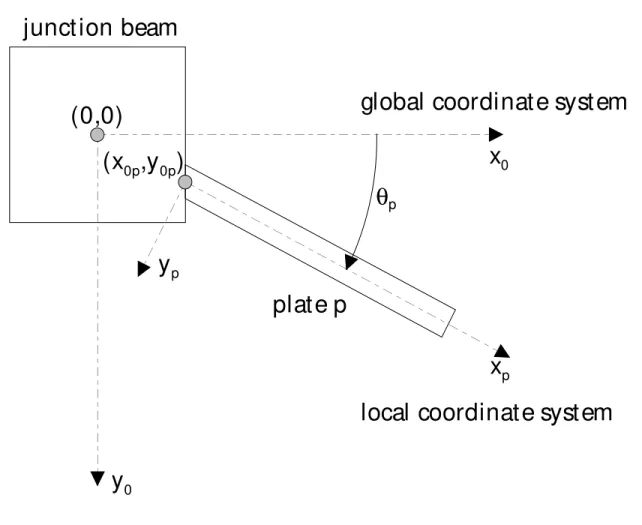
Figure 8 illustrates that each plate can be coupled at any arbitrary coupling angle. The plate orientation is characterized by θp, which represents the angle between the (x,z)-plane of the plate and
the (x,z)-plane of the global coordinate system. The eccentricity by which a plate is connected to the junction beam depends on the fixation position of the plate’s midplane (x0p,y0p).
The boundary conditions at the joint (xp=0) consist of equilibrium conditions of the junction beam
displacements of the junction beam. The equilibrium conditions, expressed in the global coordinate system, are given by:
( )
( )
(
F 0 cos F 0 sin)
0 F p p yp p xp x = θ − θ = (1)( )
( )
(
F 0 sin F 0 cos)
0 F p p yp p xp y = θ + θ = (2)( )
0 0 F F p zp z = = (3)( )
0 y(
F( )
0 cos F( )
0 sin)
x(
F( )
0 sin F( )
0 cos)
0 M M p p yp p xp p 0 p p yp p xp p 0 p zp z =− − θ − θ + θ + θ = (4)where the summations are taken over all plates. For each plate p, four continuity conditions are expressed in the local coordinate system as:
( )
b p b p zb(
0p p 0p p)
p 0 =ξ cosθ +η sinθ +α x sinθ −y cosθ
ξ (5)
( )
b p b p zb(
0p p 0p p)
p 0 =−ξ sinθ +η cosθ +α x cosθ +y sinθ
η (6)
( )
b p 0 =ζ ζ (7)( )
zb zp 0 =α α (8)For a plate strip, an additional set of boundary conditions is required for the plate edge at xp=Lx. In this
paper, free boundary conditions are assumed at the plate strip edge:
( )
L =F( )
L =F( )
L =M( )
L =0Fxp x yp x zp x zp x (9)
In the following paragraphs, the plate strip model will be elaborated by discussing the solutions to the equations of motion. Although equations will be presented only for bending waves, the same approach can be applied to in-plane waves.
A unit amplitude wave traveling with wavenumber ki and angle of incidence θi towards the junction
on one of the semi-infinite plates is described by (the time dependence ejωt is omitted):
( )cos x -jk( )sin z
jki i i e i i i
e θ θ θ θ (10)
The resulting bending wave response of a semi-infinite plate is written as:
( ) ( )
(
-jk x)
-jk( )sin z + x jk -+ z sin jk -p i i i 2 Bx 1 Bx i i i = A e +B e e e x θ θ θ θ η (11)where A+ and B+ represent the wave amplitudes, and the bending wavenumbers kBx1 and kBx2 are
derived in [16]. Equation (11) corresponds to wave propagation away from the junction, i.e. in the direction of the positive x-axis. Depending on the wavenumber and heading θi of the incident wave,
each term in (11) represents a propagating wave or a nearfield. For a plate strip, the reflection at xp=Lx
must be taken into account. In this case, the formulation of the bending wave response should include wave propagation in the direction of the positive as well as the negative x-axis:
( )
( )(
jk x)
-jk( )sin z -x jk -x jk -x jk -z sin jk -p i i i 2 Bx 2 Bx 1 Bx 1 Bx i i i A e Ae B e Be e e x θ θ = + + + + + θ θ η (12)At some frequencies, interference between both oppositely running wave components will lead to resonances and anti-resonances of the plate strip. While resonances cause a reduction of the junction impedance and consequently an increase of structure-borne sound transmission, anti-resonances lead to a significant attenuation of structure-borne sound. Since the internal loss of the plate material is not included in the analysis, one might expect singularities at resonance frequencies. However, an infinite response of the plate strip does not occur due to wave conversion and transmission to other plates.
3.3 Eccentric beam model.
In the eccentric beam model, the plate strip discussed in the previous section is omitted from the junction, and the influence of the stiffening rib is taken into account by assigning a proper mass and stiffness to the junction beam, as in the approach of Steel [8]. In this case, the junction beam will resist the forces and moments imposed by the plates and the equilibrium conditions (1)-(4) will differ from zero. The model is developed for orthotropic beams with rectangular cross-sections. The principal material directions in the beam material are assumed to be parallel to the beam axis and the edges of the cross-section.
The forces acting in the x- and y-direction of the global coordinate system (see Figure 7) will cause bending of the beam in the (x,z)- and (y,z)-planes. Shear deformation and rotatory inertia is included by modeling the beam bending using Timoshenko’s theory [17]. Bending due to a force per unit length Fx,
acting in the x-direction, is governed by the following equation of motion:
x 4 b 4 xz yy 2 2 2 b 4 xz z yy 2 b 2 y x 4 b 4 yy z F t G k I t z G k E 1 I t h h z I E = ∂ ξ ∂ ′ ρ + ∂ ∂ ξ ∂ ö çç è æ ′ + ρ − ∂ ξ ∂ ρ + ∂ ξ ∂ (13)
Here, Ez and Gxz represent the Young’s modulus in the z-direction and the shear constant
corresponding to the (x,z)-plane. The density of the beam material is symbolized by ρ, and hx and hy
denote the dimensions of the beam cross-section in the x- and y-direction. The moment of inertia Iyy is
12 h h I y 3 x yy= (14)
Timoshenko’s assumption of a uniform distribution of the shear stress over the beam cross-section requires a correction factor k′, which is taken equal to 0.833 for rectangular cross-sections. At a plate/beam junction, the beam is driven by the plates and its response is determined by the trace wavenumber ki(θi)sinθi and the time dependence ejωt imposed by the incident wave. As a consequence,
the equilibrium condition (1) is rewritten as:
( )
( )
b xz yy 2 4 xz z i 2 i 2 i 2 yy y x 2 yy z i 4 i 4 i x G k I G k E 1 sin k I h h I E sin k F ξ ö ç ç è æ ′ ρ ω + ÷÷ ö çç è æ ′ + θ θ ω ρ − ρ ω − θ θ = (15)Similarly, the equilibrium condition (2) for the forces acting in the y-direction can be derived as:
( )
( )
b yz xx 2 4 yz z i 2 i 2 i 2 xx y x 2 xx z i 4 i 4 i y G k I G k E 1 sin k I h h I E sin k F η ö ç ç è æ ′ ρ ω + ÷ ÷ ö ç ç è æ ′ + θ θ ω ρ − ρ ω − θ θ = (16)where Gyz denotes the shear constant in the (y,z)-plane and Ixx is calculated by interchanging the indices
x and y in (14).
Since a force per unit length Fz acting in the beam’s axial direction induces compression of the
beam, the response is determined by the equation of motion for quasi-longitudinal waves [18]:
z 2 b 2 2 b 2 z y x F t z E h h çç ö= è æ ∂ ζ ∂ ρ + ∂ ζ ∂ − (17)
As a result, the equilibrium condition (3) corresponding to the z-direction is rewritten as:
( )
(
)
b 2 i 2 i 2 i z y x z h h E k sin F = θ θ −ρω ζ (18)The junction beam will be subjected to torsion due to the bending moments at the plate edges. The beam response for excitation by a torsional moment per unit length Mz is governed by the following
differential equation [18]: z 2 zb 2 z 2 zb 2 M t J z T = ∂ α ∂ ρ + ∂ α ∂ − (19)
where the polar moment of inertia Jz is equal to Ixx+Iyy. The torsional stiffness is calculated as:
az b ah G
h
T=κκκκ 3 (20)
In (20), ha and hb represent the dimensions of the beam cross-section. The coefficient κ depends on the
az bz b a G G h h = σσσσ (21)
The subscripts a and b in Eqs. (20) and (21) refer to the coordinate system and correspond to either the x- or the y-direction. The subscripts should be chosen so that σ is larger than or equal to unity. In this case, κ can be estimated as a function of σ using the table given in Ref. 19. Finally, the equilibrium condition (4) for beam torsion is given as:
( )
(
)
zb 2 z i 2 i 2 i z Tk sin J M = θ θ −ρ ω α (22) 4. EXPERIMENTAL VERIFICATIONThe calculation models outlined in the previous section are verified on two different structures. Since the anisotropic and inhomogeneous character of the materials involved in realistic subfloor/joist connections may not justify the assumptions introduced in the theory, a first series of tests were performed for a rib-stiffened plate structure consisting of Plexiglas. The validation on a structure using a homogeneous and isotropic material represents an appropriate evaluation of the concepts of the plate strip and eccentric beam models. Next, the accuracy of the models for realistic materials is investigated on the subfloor/joist connection discussed in section 2.
4.1 Plexiglas structure.
The Plexiglas structure is illustrated in Figure 9. A Plexiglas sheet, measuring 2.46 x 1.22 x 0.0117 m, was suspended from the laboratory ceiling using cords and springs. A stiffening rib was attached at the center of the sheet by 17 equally spaced screws, dividing the sheet in two plates. Since glue was not used at the joint in order to preserve the integrity of the plates, the joint may not behave as a line connection at all frequencies. Three different cases were considered depending of the depth of the stiffening rib. Each rib was 1.22 m long and 0.01871 m thick, and the depth of the three ribs was taken equal to 0.05, 0.10 and 0.235 m. The material properties were taken as: Young’s modulus E = 4.8⋅109 Pa, Poisson’s ratio ν = 0.4, density ρ = 1183 kg/m3. The damping of the sheet was determined by reverberation time measurements on the suspended sheet without a rib.
The calculations were carried out using three different models of the joint. In the first model, the stiffening rib is treated as a plate strip, whereas in the second model the eccentric Timoshenko beam
theory is used. In the third approach, the joint is modeled as a classic T-joint, assuming that the stiffening rib can be considered as a plate subsystem. The coupling angles and the fixation point coordinates used in the plate strip model and the eccentric beam model are listed in Tables 1 and 2. In the T-joint model, the plate corresponding to the rib has the same coupling conditions as the plate strip in Table 1. The models were used to calculate the coupling loss factor between plates 1 and 2. The transverse velocity level difference between both plates was then estimated using SEA.
Plate element θθθθp [rad] x0p y0p
Plate 1 0 0 0
Plate 2 π 0 0
Plate strip π/2 0 h/2
Table 1: Coupling angle and fixation point coordinates used in the plate strip model (h is the thickness of plates 1 and 2).
Plate element θθθθp [rad] x0p y0p Plate 1 0 0 -(h+hy)/2
Plate 2 π 0 -(h+hy)/2
Table 2: Coupling angle and fixation point coordinates used in the eccentric beam model (h is the thickness of plates 1 and 2, hy is the
beam thickness in the y-direction).
Figure 10 shows the measured and predicted velocity level difference when the 5 cm deep stiffening rib was installed. Of all models, the plate strip results agree best with the measured data. A slight underestimation of the velocity level difference can be observed up to 1 kHz, but the pronounced peak at 1.6 kHz is accurately predicted and the theoretical results generally show a similar trend as the experimental data. At low and mid frequencies, the predictions of the eccentric beam and plate strip models are almost identical, which confirms the findings of Heron [15]. However, the eccentric beam
calculations start to deviate from the measured results above 1 kHz. Modeling the 5 cm rib as a plate subsystem is clearly inappropriate as the T-joint model overestimates the velocity level differences in almost the entire frequency range.
The pronounced maximum in Figure 10 is explained based on a few calculation examples. If the model is simplified by limiting the calculations to normal incidence and by restricting the motion of the junction beam to rotation only, then the joint behaves as a pinned junction of one finite-sized and two semi-infinite beams. In this equivalent beam junction, the finite-sized beam represents the stiffening rib and its length is equal to the depth of the rib. At a pinned joint, bending waves are transmitted exclusively by bending moments. As a result, the bending wave transmission loss will be determined by the moment impedance of the coupled beams. Since the moment impedance of the finite-sized beam is characterized by resonances and anti-resonances, the bending wave transmission loss between the two infinite beams shows a series of minima and maxima at the corresponding resonance and anti-resonance frequencies. Figure 11 shows the bending wave transmission loss for normal incidence and bending waves only for the 5 cm rib junction. Also shown is the moment impedance ZM of a pinned 5
cm long beam. It is clearly demonstrated that the distinct maximum in the transmission loss curve is located exactly at the first anti-resonance frequency of the finite-sized beam. When the joint is allowed to translate as well as to rotate, the bending wave transmission loss changes drastically as illustrated in Figure 11. The maximum corresponding to the anti-resonance is reduced significantly and its position is shifted to a lower frequency. Figure 11 shows that averaging the transmission coefficient over all angles of incidence, as was done for the plate strip model results in Figure 10, leads to a further reduction of the maximum and an additional shift to lower frequencies. This final peak corresponds to the maximum in the velocity level difference curve in Figure 10, which thus proves to be related to the anti-resonance of the stiffening rib.
Figure 12 shows the measurements and calculations for the 10 cm deep stiffening rib. Also in this case, the plate strip model agrees well with the measurements. The eccentric beam model works reasonably well at low frequencies, but starts to overestimate the velocity level difference above 1 kHz. Modeling the rib as a plate still leads to inaccurate predictions, although the agreement between the measurements and the T-joint model calculations is good at the highest one-third octave bands.
Measured and predicted results for the 23.5 cm rib are plotted in Figure 13. Except for some discrepancies at low and at high frequencies, the plate strip model produces very reliable predictions.
While the eccentric beam model is only useful up to 250 Hz, the accuracy of the T-joint model is acceptable starting from 2 kHz. After comparing Figures 10, 12 and 13 it can be concluded that increasing the depth of the rib effectively reduces the upper frequency limit below which the eccentric beam model is relatively accurate. In addition, increasing the rib depth also reduces the lower frequency limit above which the junction may be modeled as a T-joint. In general, the plate strip model seems to work well at all frequencies in all three cases and, consequently, represents the preferred calculation model in a frequency range where the stiffening rib behaves neither as a beam nor as a plate.
4.2 Subfloor/joist connection.
The calculation models were verified on the rib-stiffened structure discussed in section 2, where the joist was connected to an OSB sheet using a combination of glue and 17 screws. The elastic properties of the subfloor and the joist were determined by measuring the resonance frequencies of beam samples taken from both materials, as suggested by Hearmon [19]. Both the Young’s modulus in direction of the beam axis and the shear constant in the plane of bending could be estimated simultaneously by taking shear deformation into account. Since not all elastic constants could be determined based on these measurements, some literature data were used in the calculations. The material properties of the joist and OSB-sheet are listed in Table 3. While the internal loss factor of the joist was estimated by measuring the half-value bandwidth of the beam resonances, the damping of the OSB sheet was determined by measuring the reverberation time of the OSB sheet without the joist. The calculations were carried out using the coupling parameters given in Tables 1 and 2.
Element Ex [Pa] Ez [Pa] Gyz [Pa] Gxz [Pa] ννννxz ρρρρ [kg/m3] OSB 6.6⋅109 1.5⋅109 / 2.0⋅109 (*) 0.3 (*) 558 Joist 2.5⋅108 1.0⋅1010 8.7⋅107 1.8⋅108 5.9⋅10-4 (**) 540
Table 3: Material properties of the OSB subfloor and the joist. OSB-data (*) after Larsson [20], joist-data (**) after Illston [21].
Figure 14 shows the measured and predicted velocity level difference for the subfloor/joist junction. Although the low frequency accuracy for the plate strip model is reasonable, the underestimation of the velocity level difference above 630 Hz is unacceptably high. In addition, the calculated data do not show the same trend as the measured results since the maximum at 1600 Hz is not predicted. Figure 14 further illustrates that neither of the other two models are successful at predicting the velocity level difference at high frequencies.
In view of the good results obtained for the Plexiglas structure, the discrepancies between measurement and calculation for the realistic joint are probably caused by the anisotropic and inhomogeneous nature of the materials. One possible explanation is the fact that the influence of rotatory inertia and shear deformation was not included in the mathematical description of the plate response by virtue of the thin plate assumption. Since the measurements on the beam samples showed that shear deformation was important in both materials, the thin plate assumption is very likely to introduce prediction errors which might increase with increasing frequency. Further, the principal material directions in the joist are not parallel to the edges of the cross-section. In fact, the orthotropic structure is determined by the annular rings in the wood, and the principal directions are normal to (radial) and parallel (tangential) to these rings. This polar orthotropy can lead to coupling between the various wave types in the joist, which is not incorporated in the presented theory. An additional error might be introduced by taking part of the elastic properties from literature, as it is unclear whether these data are truly representative for the materials used in the experiments.
5. CONCLUSIONS
Vibration attenuation across a typical subfloor/joist connection was investigated experimentally and theoretically in laboratory conditions. The typical connection using equally spaced screws was studied in a series of experiments with systematic changes in the coupling conditions of the joist. It was demonstrated that structure-borne sound transmission across the joist does not depend exclusively on the spacing between the fasteners, but rather on an effective contact area between the joist and the subfloor in the vincinity of each fastener.
As a first step towards modeling flanking transmission through wood frame floors, a calculation model was developed for predicting structure-borne sound transmission between two plates coupled along a line by an eccentric stiffening rib. Three different variants of the model were considered in
which the stiffening rib was treated as a beam, a plate strip or a plate subsystem. The calculation models were verified experimentally on a Plexiglas structure as well as on a subfloor/joist connection. Three different depths of the stiffening rib were considered in the Plexiglas test series. The accuracy of the plate strip model proved to be good in all three cases and at all frequencies. It was found that the eccentric beam model is essentially the same as the plate strip model below the first anti-resonance of the stiffening rib. Modeling the connection as a classic T-joint is only acceptable at high frequencies, where the rib starts to support a sufficient number of modes. In spite of the good results for the Plexiglas structure, the agreement between measurement and calculation for the subfloor/joist connection was rather poor at mid and high frequencies for all three models. The discrepancies are assumed to be caused by the anisotropic and inhomogeneous character of the subfloor and the joist, and more research is required to investigate the effect of shear deformation and the internal structure of materials commonly used in wood frame buildings.
REFERENCES
1. Kihlman, T. 1967 Transmission of structure-borne sound through buildings. Report 9 National Swedish Institute for Building Research, Stockholm.
2. Wöhle, W., Beckmann, Th. and Schreckenbach, H. 1981 Journal of Sound and Vibration 77(3), 323-334. Coupling loss factors for statistical energy analysis of sound transmission at rectangular structural slab joints, part I.
3. Wöhle, W., Beckmann, Th. and Schreckenbach, H. 1981 Journal of Sound and Vibration 77(3), 335-344. Coupling loss factors for statistical energy analysis of sound transmission at rectangular structural slab joints, part II.
4. Craven, P.G. and Gibbs, B.M. 1981 Journal of Sound and Vibration 77(3), 417-427. Sound transmission and mode coupling at junctions of thin plates, part I : representation of the problem. 5. Gibbs, B.M. and Craven, P.G. 1981 Journal of Sound and Vibration 77(3), 429-435. Sound
transmission and mode coupling at junctions of thin plates, part II : parametric survey.
6. Craik, R.J.M. 1982 Journal of Sound and Vibration 82(4), 505-516. The prediction of sound transmission through buildings using statistical energy analysis.
7. Steel, J.A. and Craik, R.J.M. 1993 Applied Acoustics 39(1993), 191-208. Sound transmission between columns and floors in framed buildings.
8. Steel, J.A. 1994 Journal of Sound and Vibration 178(3), 379-394. Sound transmission between plates in framed structures.
9. Craik, R.J.M., Nightingale, T.R.T. and Steel, J.A. 1997 Journal of the Acoustical Society of
America 101(2), 964-969. Sound transmission through a double leaf partition with edge flanking.
10. Bosmans, I., Mees, P. and Vermeir, G. 1996 Journal of Sound and Vibration 191(1), 75-90. Structure-borne sound transmission between thin orthotropic plates: analytical solutions.
11. Bosmans, I. and Vermeir, G. 1997 Journal of the Acoustical Society of America 101(6), 3443-3456. Diffuse transmission of structure-borne sound at periodic junctions of semi-infinite plates. 12. Craik, R.J.M. and Smith, R.S. Accepted for publication in Applied Acoustics Sound transmission
through lightweight plasterboard walls. Part II: structure-borne sound (1998).
13. Craik, R.J.M. 1982 Applied Acoustics 15, 355-361. The measurement of structure-borne sound transmission using impulsive sources.
14. Langley, R.S. and Heron, K.H. 1990 Journal of Sound and Vibration 143(2), 241-253. Elastic wave transmission through plate/beam junctions.
15. Heron, K.H. 1997 Predictive SEA using line wave impedances. In: Fahy, F.J. and Price, W.G. (Eds.) 1999 IUTAM Symposium on Statistical Energy Analysis, 107-119. Dordrecht, Kluwer. 16. Bosmans, I. 1998 Analytical modeling of structure-borne sound transmission and modal
interaction at complex plate junctions. Ph.D. Dissertation, K.U.Leuven (ISBN 90-5682-131-8). 17. Weaver, W., Timoshenko, S.P. and Young, D.H. 1990 Vibration problems in engineering. New
York, Wiley, fifth edition.
18. Cremer, L., Heckl, M. and Ungar, E.E. 1988 Structure-Borne Sound. Berlin, Springer-Verlag, second edition.
19. Hearmon, R.F.S. 1966 Forest Products Research Society, 16(8), 29-40. Vibration Testing of Wood.
20. Larsson, D. 1997 Journal of Engineering Mechanics, 123(3), 222-229. Using modal analysis for estimation of anisotropic material constants.
FIGURE CAPTIONS
Figure 1: Cross-section of a joint between two walls and a floor/ceiling assembly. The subfloor is supported by a series of parallel wood joists.
Figure 2: One joist was screwed against an OSB sheet and mounted on a resilient layer on the laboratory floor. The structure was kept upright by two strings.
Figure 3: In the first series of tests, the joist was attached directly to OSB sheet (a), whereas in the second series square aluminum spacers are used to create a well-defined contact area (b).
Figure 4: Measured velocity level difference as a function of frequency for the cases where the joist was directly attached to the OSB sheet: line connection (), 17 screws (∆), 9 screws (Ο) and 5 screws ( ).
Figure 5: Measured velocity level difference as a function of frequency for the cases where aluminum spacers were used to create a well-defined contact area between the joist and the OSB sheet: line connection (), 17 spacers (∆), 9 spacers (Ο) and 5 spacers ( ).
Figure 6: Eccentric beam model: rigid body motion (a). Plate strip model: cross-section deformation (b).
Figure 7: Model of the junction: conventions of forces and displacements.
Figure 8: Plates can be connected at any arbitrary coupling angle θp . The eccentricity of the joint is
determined by the coordinates of the fixation point (x0p,y0p).
Figure 9: The Plexiglas structure was suspended from the laboratory ceiling using cords and soft springs. Three different cases were considered depending on the depth of the stiffening rib. The ribs were attached to the plate using 17 equally spaced screws (spacing 7.5 cm).
Figure 10: Measured and predicted velocity level difference for the Plexiglas structure with a 5 cm deep stiffening rib: measured (∆), plate strip model (), eccentric beam model (---) and T-joint (⋅⋅⋅⋅⋅⋅⋅).
Figure 11: Calculated transmission loss for the Plexiglas structure with a 5 cm deep stiffening rib: normal incidence bending wave only (), normal incidence bending and in-plane waves (---), random incidence bending and in-plane waves (⋅⋅⋅⋅⋅⋅⋅). Calculated moment impedance ZM of a 5 cm
long, 1.871 cm thick Plexiglas beam (-⋅-⋅-⋅-⋅).
Figure 12: Measured and predicted velocity level difference for the Plexiglas structure with a 10 cm deep stiffening rib: measured (∆), plate strip model (), eccentric beam model (---) and T-joint (⋅⋅⋅⋅⋅⋅⋅).
Figure 13: Measured and predicted velocity level difference for the Plexiglas structure with a 23.5 cm deep stiffening rib: measured (∆), plate strip model (), eccentric beam model (---) and T-joint (⋅⋅⋅⋅⋅⋅⋅).
Figure 14: Measured and predicted velocity level difference for the subfloor/joist connection: measured (∆), plate strip model (), eccentric beam model (---) and T-joint (⋅⋅⋅⋅⋅⋅⋅).
1
2
3
4
5
6
7
2
2
3
3
7 6
1. OSB subfloor
2. W ood joist s
3. Cross-bridging
4. Resilient channels
5. Gypsum board ceiling
6. Gypsum board wall
7. W ood studs
Figure 1: Cross-section of a joint between two walls and a floor/ceiling assembly. The subfloor is supported by a series of parallel wood joists.
resilient layer
string
st ring
1
2
joist
Figure 2: One joist was screwed against an OSB sheet and mounted on a resilient layer on the laboratory floor. The structure was kept upright by two strings.
a)
b)
L
screws
L
spacers
Figure 3: In the first series of tests, the joist was attached directly to OSB sheet (a), whereas in the second series square aluminum spacers are used to create a well-defined contact area (b).
125 250 500 1000 2000 4000 2 4 6 8 10 12 14 16 18 2 1 V eloci ty L evel D if fer ence [ d B] Frequency [Hz]
Figure 4: Measured velocity level difference as a function of frequency for the cases where the joist was directly attached to the OSB sheet: line connection (), 17 screws (∆), 9 screws (Ο) and 5 screws ( ).
125 250 500 1000 2000 4000 2 4 6 8 10 12 14 16 18 spacers 2 1 V elo ci ty L ev el D iff er en ce [ d B ] Frequency [Hz]
Figure 5: Measured velocity level difference as a function of frequency for the cases where aluminum spacers were used to create a well-defined contact area between the joist and the OSB sheet: line connection (), 17 spacers (∆), 9 spacers (Ο) and 5 spacers ( ).
a)
b)
Figure 6: Eccentric beam model: rigid body motion (a). Plate strip model: cross-section deformation (b).
xp yp zp Fyp Fxp Fzp Mzp αzp ηp ζp ξp αzb ηb ζb ξb
semi-infinite plate semi-infinit e plate
junct ion beam
plat e strip Lx x0
y0
z0
x
0y
0y
px
p(x
0p,y
0p)
θ
pglobal coordinate system
local coordinate system
plate p
junction beam
(0,0)
Figure 8: Plates can be connected at any arbitrary coupling angle θp . The eccentricity of the joint is
cord
spring
17 equally spaced screws
ceiling
1
2
Figure 9: The Plexiglas structure was suspended from the laboratory ceiling using cords and soft springs. Three different cases were considered depending on the depth of the stiffening rib. The ribs were attached to the plate using 17 equally spaced screws (spacing 7.5 cm).
125 250 500 1000 2000 4000 4 6 8 10 12 14 16 18 20 22 2 1 V elo ci ty L ev el D iff er en ce [ d B ] Frequency [Hz]
Figure 10: Measured and predicted velocity level difference for the Plexiglas structure with a 5 cm deep stiffening rib: measured (∆), plate strip model (), eccentric beam model (---) and T-joint (⋅⋅⋅⋅⋅⋅⋅).
50 100 200 400 800 1600 3200 0 10 20 30 40 50 60 70 2 1 Anti-resonance Frequency [Hz] T ra n sm issi o n L o ss [ d B ] -60 -50 -40 -30 -20 -10 0 10 20 30 40 50 60 ZM M o m ent I m p ed anc e Z M [ d B , re 1 N m s/rad]
Figure 11: Calculated transmission loss for the Plexiglas structure with a 5 cm deep stiffening rib: normal incidence bending wave only (), normal incidence bending and in-plane waves (---), random incidence bending and in-plane waves (⋅⋅⋅⋅⋅⋅⋅). Calculated moment impedance ZM of a 5 cm
125 250 500 1000 2000 4000 4 6 8 10 12 14 16 18 20 22 24 2 1 V elo ci ty L ev el D iff er en ce [ d B ] Frequency [Hz]
Figure 12: Measured and predicted velocity level difference for the Plexiglas structure with a 10 cm deep stiffening rib: measured (∆), plate strip model (), eccentric beam model (---) and T-joint (⋅⋅⋅⋅⋅⋅⋅).
125 250 500 1000 2000 4000 4 6 8 10 12 14 16 18 20 22 24 26 28 2 1 V elo ci ty L ev el D iff er en ce [ d B ] Frequency [Hz]
Figure 13: Measured and predicted velocity level difference for the Plexiglas structure with a 23.5 cm deep stiffening rib: measured (∆), plate strip model (), eccentric beam model (---) and T-joint (⋅⋅⋅⋅⋅⋅⋅).
125 250 500 1000 2000 4000 3 6 9 12 15 18 21 24 27 30 2 1 V elo ci ty L ev el D iff er en ce [ d B ] Frequency [Hz]
Figure 14: Measured and predicted velocity level difference for the subfloor/joist connection: measured (∆), plate strip model (), eccentric beam model (---) and T-joint (⋅⋅⋅⋅⋅⋅⋅).

![Table 3: Material properties of the OSB subfloor and the joist. OSB-data (*) after Larsson [20], joist- joist-data (**) after Illston [21].](https://thumb-eu.123doks.com/thumbv2/123doknet/14206950.481163/15.918.130.782.825.928/table-material-properties-subfloor-joist-larsson-joist-illston.webp)