Cavity quantum electrodynamics with ensembles of ytterbium-171

(1)

Cavity Quantum Electrodynamics with Ensembles of

Ytterbium-171

by

Boris Braverman

B.Sc., University of Toronto (2011)

Submitted to the Department of Physics

in partial fulfillment of the requirements for the degree of

Doctor of Philosophy in Physics

at the

MASSACHUSETTS INSTITUTE OF TECHNOLOGY

February 2018

c

○ 2018 Massachusetts Institute of Technology. All rights reserved.

Author . . . .

Department of Physics

January 24, 2018

Certified by. . . .

Vladan Vuletić

Lester Wolfe Professor of Physics

Thesis Supervisor

Accepted by . . . .

Scott Hughes

Professor of Physics

Interim Associate Department Head

(2)

(3)

Cavity Quantum Electrodynamics with Ensembles of

Ytterbium-171

by

Boris Braverman

Submitted to the Department of Physics on January 24, 2018, in partial fulfillment of the

requirements for the degree of Doctor of Philosophy in Physics

Abstract

In this thesis, I present the realization of a system applying the tools of cavity quantum electrodynamics to an atomic optical lattice clock.

We design and implement a unique experimental cavity structure, with a small radius of curvature mirror on one side and a large mirror on the other side. With this structure, we are able to probe ytterbium-171 atoms in both the weak and strong coupling regimes of cavity quantum electrodynamics. This asymmetric micromirror structure simultaneously offers strong light-atom coupling, mechanical robustness, and excellent access to a large cavity volume.

We develop a simple but accurate model for strong light-atom interactions in our system, which allows us to predict the performance of both cavity-assisted quantum nondemolition measurements of the atomic state, and the back-action of the probing light onto the atomic state.

We find theoretically, and confirm experimentally, that probing the atom-cavity system with two frequencies at the vacuum Rabi peaks of a system with strong col-lective light-atom coupling generates the largest possible entanglement between the probing light and the atomic state. With this scheme, we demonstrate atomic number measurements within a factor of 2 of the quantum Fisher information limit.

By using the quantum back-action of the probing light on the atomic ensemble, we perform squeezing by cavity feedback. We produce states with −11±1 dB of variance squeezing and 14±1 dB of antisqueezing. Using theoretical simulations, we show that states with near-unitary squeezing offer significant advantages for improving atomic clocks compared to previous work.

The ability to load large atomic ensembles in the strong coupling regime in our system offers several routes to the generation of highly entangled non-Gaussian quan-tum states. Such states can be produced by heralded measurements, or by global atom-atom interactions based on unitary spin squeezing.

Altogether, we realize a system of unprecedented versatility and great potential for performing a large variety of hybrid atomic clock and cavity QED experiments.

(4)

Thesis Supervisor: Vladan Vuletić Title: Lester Wolfe Professor of Physics

(5)

Acknowledgments

The results I describe in my thesis are the product of years of work by the talented and hard-working team of the Yb Clock project in the group of Vladan Vuletić. Vladan is a wonderful role model – always a source of optimism and thoughtful guidance, with no question too big or too small to discuss and analyze. I have learned a great deal from his deep insights on everything, from quantum mechanics and atom-light interactions to feedback loops and lasers, a depth and breadth of knowledge that I hope to reach someday.

Akio Kawasaki and I worked side by side for 6 years, building from an empty room all the way to the experiment as it is today. His drive to tackle any challenge and move the experiment forward have been invaluable. Over the years, Akio and I were joined by many capable colleagues that left indelible marks on the experiment. Özge Özel joined us at the start and set up much of our efficient lab infrastructure. David Levonian and Daisuke Akamatsu contributed tremendously to building and locking narrow lasers. André Heinz built and characterized our stable reference cavity. Grace Zhang was the driving force behind our 3-D printed shutter project. Enrique Mendez introduced many innovations in digital electronics and circuit design and construction. We benefited greatly from the hard work of other lab members as well: David Ma, Leonardo Salvi, Christopher Sanfillipo, Yasunari Suzuki, Tamara Sumarac, Sophie Weber, Tailin Wu, Yanhong Xiao, Megan Yamoah, QinQin Yu, Harry Zhou, and Bojan Zlatković. As I near the end of my time at MIT, I am confident that the future of the experiment is bright, in the capable hands of the new generation: Edwin Pedrozo, Chi Shu, Simone Colombo, and Zeyang Li.

The entire Vuletić group and the Center for Ultracold Atoms were a generous source of technical wisdom, scientific insights, and necessary equipment. I learned a tremendous amount about topics ranging from quantum measurement to low-noise laser electronics and vacuum systems from Kristin Beck, Dorian Gangloff, Alexei Bylinskii, Mahdi Hosseini, Hao Zhang, Jesse Amato-Grill, Michael Gutierrez, Wenlan Chen, Jeff Thompson, and many others. Sometimes, I needed to venture outside the

(6)

CUA to get things done for the project, and MIT staff were there to help: Mark Belanger taught me a great deal about machining metal, plastics, and ceramics, while Kurt Broderick taught me everything I needed to know about nanofabrication.

I am grateful for my friends outside of the lab, Daniel Kolodrubetz, Colin Kennedy, Reed Essick, Fabián Kozynski, Rachael Harding, Steven Chang, Bernhard Zimmer-mann, George Chen, Frank Wang, Stephanie Nam, William Li, Jenny Wang, and many others, who made my time at MIT enjoyable through many meals together and a shared appreciation for puzzles, art, and nature. The MIT Physics Department fos-tered a warm atmosphere, and I am especially grateful for the wonderful community at Sidney-Pacific and all the great times I’ve had there.

Most of all, I have to thank my loving and supportive family: Elena, Leonid, Mark, Anna, and Linda. Every day, you remind me that there are things in life more beautiful than even a smoothly running experiment. You have sacrificed a great deal along my PhD journey, and at the end of it all, I hope that I’ve made you proud.

(7)

List of Figures

1-1 Ramsey spectroscopy measures the phase difference between a local oscillator and the atoms’ frequency, allowing for the construction of atomic clocks. . . 34 1-2 Stability of several generations of 133_Cs _{clocks at NIST. This figure is}

adapted from [94]. . . 35 1-3 A summary plot of recent state of the art clocks using different atomic

species. Red circles, blue squares, and green triangles correspond to hyperfine fountain clocks, single-ion optical clocks, and optical lattice clocks respectively. . . 37 1-4 Accurate clock comparisons enable measurements of the time variation

of dimensionless constants of nature, such as the fine structure constant 𝛼 and the proton-to-electron mass ratio 𝜇. This figure is from [69]. . . 42 1-5 Ramsey spectroscopy using a squeezed spin state reduces the projection

noise of the final measurement and improves the overall clock precision. 44 1-6 The current state of the art in spin squeezing experiments. Black,

red, and blue markers correspond respectively to trapped ions, BECs, and cold thermal atoms. Stars correspond to directly measured phase sensitivity gains, found from a complete Ramsey sequence. Circles correspond to potential sensitivity gain inferred from a characterization of the state; filled (open) circles correspond to results without (with) subtraction of technical noise. This figure is from [117]. . . 47

(14)

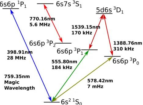
2-1 Simplified level diagram of the lowest energy levels of 171_Yb_{. Hyperfine}

structure is not shown. . . 54 2-2 Schematic diagram of atoms in an optical cavity, illustrating the

self-consistency condition for the cavity field – in equilibrium, the field must be constant after one round trip. Therefore, the sum of the input field 𝑖𝑡1𝐸𝑖𝑛, the radiation of the atomic ensemble 𝐸𝑀, and the cavity

field returning after the round trip 𝐸𝐶𝑟1𝑟2𝑒2𝑖𝑘𝐿 must equal the cavity

field 𝐸𝐶 itself. . . 56

2-3 A cavity with lossy mirrors is shown in (a), while an equivalent con-figuration of a lossless cavity with additional output coupling loss is shown in (b). This equivalence holds if the starred variables take the values given in (2.16). . . 60 2-4 (a) Schematic of a cQED experiment with atoms in an arbitrary

mag-netic field. (b) Level diagram for the 1_𝑆

0(𝐹 = 1/2) → 3𝑃1(𝐹 = 3/2)

transition in171_Yb_{. . . .} ₆₅

2-5 Clebsch-Gordan coefficients for the1_𝑆

0 →3𝑃1transition in171Yb. Note

that the hyperfine interaction that allows the 1_𝑆

0 → 3𝑃0 transition

has the form 𝐻 ∝ ⃗𝐼 · ⃗𝐽, which commutes with 𝐹2_{. Therefore, the}

Clebsch-Gordan coefficients for the 1_𝑆

0(𝐹 = 1/2) → 3𝑃0(𝐹 = 1/2)

clock transition are the same as the ones for 1_𝑆

0(𝐹 = 1/2) →3𝑃1(𝐹 =

1/2). The coefficients for 𝐹 = 3/2 stay the same when we replace 𝑚𝐹 → −𝑚𝐹, while those for 𝐹 = 1/2 change sign. . . 65

2-6 Simulation results for 171_Yb atoms in our experimental cavity with

zero applied magnetic field, showing the transmission intensity 𝑇𝑖 and

phase 𝜑𝑖 for the two cavity polarization eigenmodes, as well as the

Stokes vector parameters ⃗𝑆1 for the first eigenmode. (a-e) show the

cavity response for atom number 𝑁↑𝜂 = {0, 1, 10, 100, 1000} polarized

(15)

2-7 Simulation results for a specific possible cQED experiment. We input light polarized along ^𝑥 into a cavity with 𝑁↑𝜂 = 1000 atoms polarized

along ^𝑧. (a) shows the overall response – the probabilities that an input photon will be transmitted (𝑇 ), reflected (𝑅), scattered by the mirrors into free space (𝑆𝑚) or scattered by the atoms into free space (𝑆𝑎).

(b) and (c) show the Stokes vector components of the reflected and transmitted light. (d) is similar to (a), but shows the relative prob-abilities of possible outcomes (transmission and free space scattering) for a photon that is not reflected from the cavity. . . 79 2-8 Simulation results for interactions between 171_Yb _{atoms in our}

exper-imental cavity with a typical applied magnetic field ⃗𝐵 = 14 G ^𝑧. It is clear that in this configuration, the behavior of the system closely approximates an atom with only two energy levels. (a-c) show the system’s behavior for 𝑁↑𝜂 = {100, 1000, 5000}. (d) is similar to (c),

but with the addition of a large atomic population in the |↓⟩ state of 𝑁↓𝜂 = 5000. . . 81

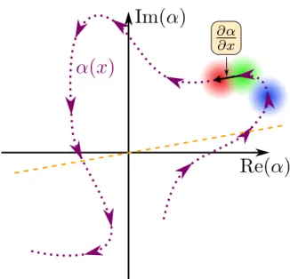
2-9 Simulation results for probing the atom-cavity system with a trans-verse applied magnetic field ⃗𝐵 = 2 G ^𝑥, showing the effect of atomic coherence on the response of the system. (a) and (b) show the effect due to a shift in the relative phase of the populations in the |↑⟩ and |↓⟩ states, while (a), (c), and (d) show the effect of going from a coherent atomic state to a statistical mixture with no coherence. . . 83 2-10 Schematic diagram of the measurement of a parameter 𝑥 by detecting

a coherent state of light 𝛼. . . 85 2-11 Conceptual illustration of two-color measurement: our goal is to

simul-taneously probe both vacuum Rabi peaks of a cQED system. . . 94 2-12 Geometric illustration of two-color probing. The single-frequency

co-herent states 𝛼 and 𝛽 add with a time-varying relative phase 𝜑 = 𝑡Δ𝜔 to give the total field 𝛾 = 𝛼 + 𝛽𝑒𝑖𝜑_{. . . .} ₉₅

(16)

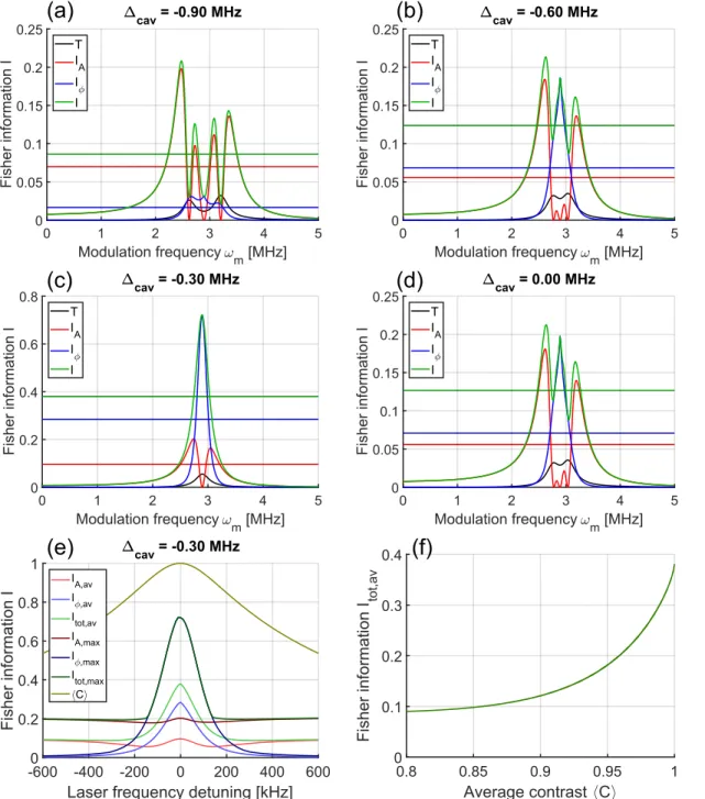
2-13 Calculations of the FI for 𝑁↑ measurement using two-color probing

with 𝑁↑𝜂 = 𝑁↓𝜂 = 500 and ⃗𝐵 = 7.5 G ^𝑧. ℐ = 1 corresponds to a

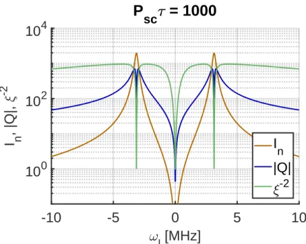
variance of 𝑁/𝜂 per photon. . . 97 2-14 Shearing strength 𝑄, Fisher information ℐ𝑡𝑜𝑡,𝑛, and net squeezing 𝜉−2

for cavity feedback squeezing with 𝑁 = 1000, 𝜂 = 1. . . 102 2-15 Illustration of a Ramsey sequence using a spin squeezed state. . . 105 2-16 Theoretical response curve for the measured atomic signal 𝑆𝑧as a

func-tion of the phase deviafunc-tion of the local oscillator 𝛿𝜑, for a clock using 1000atoms and (a) a coherent spin state (b) a squeezed spin state with 𝜉2 _{= −15 dB}. . . 107

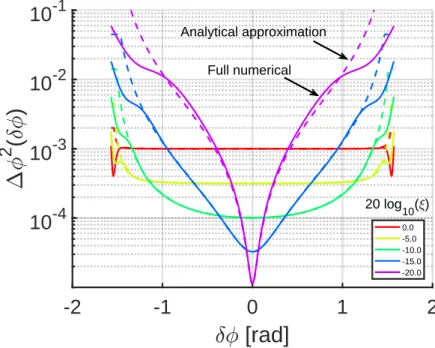
2-17 Error in the estimate of 𝛿𝜑 for different amounts of squeezing 𝜉 and actual values of 𝛿𝜑. Dashed lines are the analytical formula built from (2.95), (2.99), and (2.100), while the solid lines are the result of a numerical calculation. . . 110 2-18 (a) Phase error after one Ramsey experiment Δ2

𝜑 for different levels

of contrast 𝐶 in a clock with no squeezing, as a function of the phase deviation 𝛿𝜑. (b) Corresponding clock stability after a time 𝑇 = 𝛾−1_.

(c) Same as (a), but for perfect contrast 𝐶 = 1 and different amounts of squeezing in dB. (d) Corresponding clock stability after a time 𝑇 = 𝛾−1_.

(e) Same as (c), fixing the squeezing at 𝜉2 _{= −10 dB}_{, and varying the}

state area 𝐴 and correspondingly the antisqueezing 𝜒 = 𝐴/𝜉. (f) Corresponding clock stability. . . 112 2-19 Plot of the best possible clock performance, in units of dB of clock

phase variance, and compared to a clock with no squeezing and perfect contrast. We vary the the clock contrast and amount of squeezing, assuming no excess antisqueezing (i.e. the area of the state is 𝐴 = 1). 114 2-20 Plot of the best possible clock performance, in units of dB of clock

phase variance compared to a clock with no squeezing and perfect con-trast. We vary the the amount of squeezing, and excess antisqueezing, assuming no contrast loss, i.e. 𝐶 = 1. . . 115

(17)

2-21 Illustration of spin carving; this is Fig. 1 from [25]. . . 118 2-22 Spherical Wigner functions [143] corresponding to Schrödinger cat states

of different magnitude. These states could be produced by spin carving [25] in a cQED system of sufficiently high cooperativity 𝜂. . . 118 2-23 Plots of spherical Wigner functions [143] for different squeezing

Hamil-tonians, discussed in Section 2.9.2. Red and blue color correspond to positive and negative Wigner function values. (l) is a plot of the Husimi Q function for the same state as (k). . . 122 3-1 Stability diagram showing possible combinations of two spherical

mir-rors that can create an optical cavity. Text indicates the cavity length 𝐿 corresponding to each possible cavity arrangement. . . 129 3-2 (a) Expected waist sizes 𝑤0 and (b) single-atom cavity cooperativities

𝜂 as a function of cavity length 𝐿. These calculations are made for a cavity with one mirror of fixed ROC 𝑅1 = 25 mm and a second mirror

of a smaller curvature 𝑅2. . . 129

33 The optical axis determines the direction of the modes in the cavity -a longer optic-al -axis m-akes -a c-avity more st-able -ag-ainst mis-alignment. 130 3-4 Plot of the optical axis length necessary to attain a cooperativity of 𝜂 =

40in a cavity of finesse 14000, with one mirror of ROC 𝑅1 = 25 mm,

as a function of the ROC of the second mirror 𝑅2. A smaller value of

𝑅2 gives a larger optical axis length, making it easier to assemble the

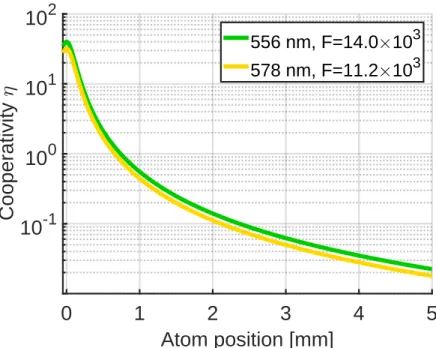
cavity and keep it aligned. . . 132 3-5 Expected single-atom cooperativity at the standing wave antinodes in

the asymmetric micromirror cavity, as a function of the atom position relative to the cavity waist. . . 135 3-6 Conceptual diagram of our finesse measurement technique. We

gener-ate clean ringdown signals by using an AOM to quickly modulgener-ate the laser beam on and off. . . 139

(18)

3-7 Typical cavity ringdown measurement data taken with a setup as shown in Figure 3-6. (a)–(c) show the APD voltage over different time spans, including an exponential decay fit in (c). (d) is a histogram of 6500 similar measurements, showing a measurement repeatability at a 0.5% level. . . 140 3-8 Overview of the major structural elements of the experimental cavity

with an asymmetric structure, with a micromirror on the top and a 25 mmmirror on the bottom. . . 142

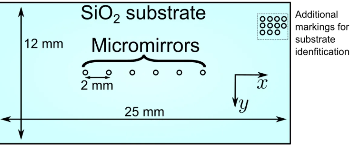
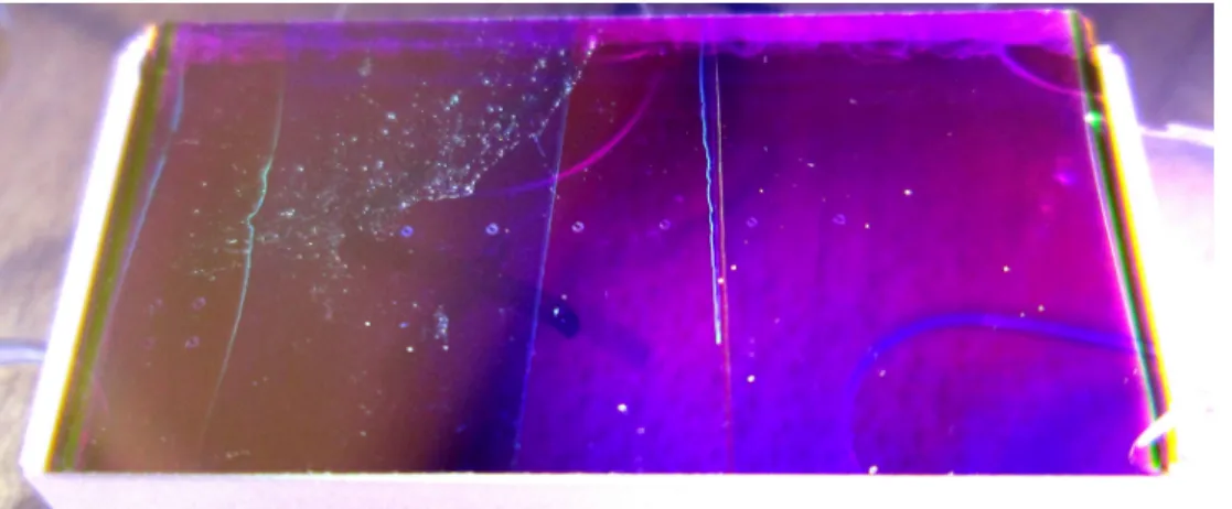
3-9 General layout of micromirror substrates used in the experiment. . . . 146 3-10 Photograph of a typical micromirror substrate. Vertical lines are

mark-ings due to dielectric coating etching (see Section 3.4.5). . . 147 3-11 Optical microscope images of three representative micromirrors from

different substrates. Mirror (b) is the one actually used in our experi-mental cavity. . . 147 3-12 Surface profiles of the micromirror used in the experiment (photograph

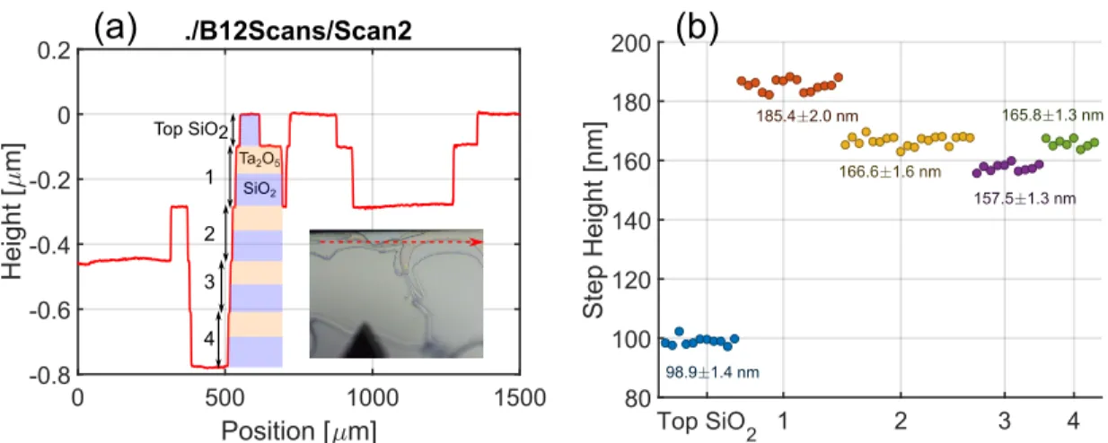
shown in Figure 3-11(b)). Plots (a) and (b) show an overview of the surface profile, which is slightly asymmetric (a feature also visible in the photograph). Plots (c) and (d) magnify the central parts of the surface profiles and show quadratic fits with typical RMS residual roughness of 1 nm, limited only by the profilometer’s stability. . . 148 3-13 (a) Example cross-section scan across a micromirror substrate that was

intentionally etched in a non-uniform way to reveal sections with dif-ferent number of etched layers. (b) Summary of several measurements such as in (a), revealing with good accuracy the thicknesses of the dielectric layers composing the high reflectivity coating. . . 153

(19)

3-14 (a) Theoretical calculation of the impact of micromirror etching on dielectric coating transmission, and resulting effect on finesse, assum-ing no change in loss. For each SiO2 and Ta2O5 layer removed, the

transmission increases by a factor of 2.13. (b) Measured micromirror coating transmission for different number of layers etched away. The transmission in fact increases by a factor of 1.92 ± 0.07 for each Ta2O5

and SiO2 layer removed. . . 154

3-15 Temperature vs. time curve for the thermal annealing of the micromir-ror used in the experimental cavity. . . 156 3-16 Effects of annealing and deposition steps on the (a) cavity finesse and

(b) light loss at the micromirror. Annealing in performed in air at 450∘C. Curves correspond to individual micromirrors on a single sub-strate. . . 156 3-17 (a) front and (b) back photographs of the micromirror substrate that

is incorporated into our science cavity. . . 157 3-18 Summary of the testing and characterization of approximately 100

mi-cromirrors. In (a-c), points of the same color correspond to micromir-rors on the same rectangular substrate. (a) Radii of curvature in the ^𝑥 and ^𝑦 directions. Our mirrors typically have astigmatism of 20%, and a manufacturing repeatability on one substrate of 20%. (b) Depth of mirror versus the geometric mean radius of curvature. As expected, deeper mirrors are more curved. (c) Best finesse seen in testing versus the geometric mean radius of curvature. There seems to be a broad peak centered around 𝑅2 = 500 𝜇m. Round markers correspond to

mirrors with no etching, while square ones are for mirrors with some etching steps. (d) Cooperativity at the cavity waist (calculated from finesse) versus the geometric mean radius of curvature. Colors indicate the transmission to loss ratio for each micromirror, with the arrow in-dicating the effect for the micromirror we are currently using in the experimental cavity. . . 160

(20)

3-19 Finesse of an asymmetric micromirror cavity as a function of transverse alignment. Inset are diagrams illustrating the formation of a cavity mode with two reflections from the micromirror substrate – once from the micromirror itself, and once from a flat region of the substrate. Note that the finesse actually equals half the plotted value outside the central region, because the FSR of the cavity is twice as large in that case. . . 161 3-20 (a) Free spectral range and (b) finesse of a cavity consisting of a 25 mm

mirror and the micromirror we are using in the experiment. The effec-tive curvature of the larger mirror depends on the cavity length due to corrections to the paraxial approximation, while the finesse degrades as the cavity gets longer due to coupling to higher order transverse modes [11]. . . 164 3-21 Top and bottom base plates used to hold the mirrors, ready for mirrors

to be glued onto them. . . 166 3-22 The (a) 25 mm mirror and (b) micromirror substrates being epoxied

onto their respective holding structures. . . 166 3-23 Temperature vs. time curve for the thermal curing of the epoxies used

in cavity assembly. These particular data are from the final epoxy-ing step – attachepoxy-ing the micromirror substrate to the two rectangular piezos that hold it in place and actuate its motion. . . 168 3-24 Wiring diagram for the 19 pins of the MiL-C-26482 feedthrough, shown

looking toward the feedthrough both from the air and vacuum sides. 169 3-25 Photograph of the two cavity base plates on a hot plate, showing the

wiring of the PZTs and the wire strain relief. . . 171 3-26 Photograph of the final state of the cavity inside the vacuum chamber,

(21)

3-27 Finesse of experimental cavity for higher order TEM𝑙,𝑚 transverse

modes. Error bars are approximately ±0.1 × 103, too small to show.

The inset figures are calculated TEMl,mmode patterns to illustrate the

spatial orientation of the measured modes. . . 174 3-28 Apparatus for measuring the complex field amplitude of the cavity

field, which is essential for optimizing mode matching into a single mode fiber. . . 175 3-29 CCD images showing steps in measuring the complex field of the cavity

mode. (a) Cavity mode intensity distribution. (b) Reference beam intensity. (c), (d) Example interference images between the cavity mode and reference beam. (e) Zoomed-in image of the cavity mode. (f), (g) Intensity and phase profiles of cavity mode, reconstructed from the interference pattern. . . 177 3-30 (a) Measured and best fit electric distributions for the experimental

cavity mode at 556 nm at the bottom of the vacuum chamber. (b) Example calculations of Gaussian beam propagation used to optimize mode matching of the cavity light to a single-mode fiber. . . 178 3-31 Long-term record of the temperature stability of the experimental

cav-ity, over approximately 2 months. (a) Cavity temperature as a function of date. The temperature transients correspond to the tuning on and off of the MOT coils, which heat the vacuum chamber surrounding the cavity. (b) Histogram of experimental cavity temperature. In the absence of MOT coil operation, the stability has a FWHM of 56 mK. (c) Heater current necessary to maintain the cavity temperature at 29.15∘C. (d) Histogram of heater currents. . . 179 3-32 (a) Schematic diagram illustrating how a change Δ𝐿 in the relative

length of the cavity posts produces a shift Δ𝑥𝑅𝑂𝐶 in the ROC center

of the 25 mm mirror. (b) Results of a finite-element simulation using only one of four heaters to heat the experimental cavity structure. . 181

(22)

3-33 Change in cavity loss as a function of transverse motion of the center of curvature of the 25 mm mirror. . . 182 3-34 The experimental cavity resonance at 556 nm shifts due to changes in

the cavity heating, even if its length is locked at 759 nm. Different colors correspond to different dates in 2017. . . 183 3-35 (a) Setup for measuring birefringent eigenmode splitting of our

ex-perimental cavity. (b) The real-space orientation of the polarization modes that the cavity light is projected onto, overlaid on the image of the micromirror used in the experimental cavity. . . 186 3-36 (a) Example plot showing the cavity transmission and Lorentzian fits

measured for polarization modes for a projection basis angled at 𝜃 = 0∘

to {^𝑥, ^𝑦}, with red and blue markers corresponding to modes with ⃗𝐸 ‖ ^𝑥 and ⃗𝐸 ‖ ^𝑦 respectively. (b) Plot summarizing about 100 measurements such as shown in (a) performed for different projection bases. . . 187 3-37 (a) Example traces showing the effect of the analysis polarization basis

on the shape of the cavity ringdown signal, an important side-effect of cavity birefringence. Note that this is a log-linear plot. (b) The inferred cavity finesse has a strong dependence on the measurement polarization, requiring special care to avoid systematic errors. . . 190 3-38 The transmission of the experimental cavity becomes bistable as we

input an increasing amount of 556 nm light. . . 191 4-1 Overview of the main vacuum chamber. Thin black lines outline the

optics table, breadboards, and 1.5 in steel pillars that connect them. . 194 4-2 View of the central part of the main vacuum chamber, near the

exper-imental cavity. . . 195 4-3 Theoretical oven flux and measured MOT loading rate, normalized to

(23)

4-4 Diagram of the in-vacuum heated window we use to prevent Yb depo-sition from attenuating the longitudinal cooling beam. This figure is adapted from [73, Sec. 4.4]. . . 197 4-5 Record of a typical single run of the titanium sublimation pump. . . . 199 4-6 Error signals for locking the 399 nm laser to the1_𝑆

0 →1𝑃1 transition in

ytterbium. Labels indicate the isotope and total angular momentum 𝐹 . 202 4-7 Frequencies relevant to locking of the 556 nm laser. Note that all

fre-quencies are in MHz and in the IR (1112 nm). This figure is adapted from [73, Fig. 5-7]. . . 204 4-8 Measurement of the linewidth of the 556 nm laser by comparison with

a 40 ± 2 kHz wide reference cavity. (a) and (b) show the transmission of the laser through the cavity with and without the “fast feedback” respectively. (c) shows the transmission of the laser when fixed on the slope of the cavity, and (d) is the corresponding histogram. With the fast feedback, we estimate a laser linewidth of 2.3 ± 0.1 kHz. . . 206 4-9 Measurement of the spectral purity of the 556 nm laser by comparison

with (a-b) a 40 kHz wide reference cavity, measured with strong light and an APD, and (c-d) the 430 kHz wide reference cavity, measured with very weak probing light and detected with an SPCM. . . 207 4-10 Schematic of the electronics and RF circuit used to generate all the

probing light used in our cQED experiments. . . 209 4-11 Overview of the 1157 nm laser system used to produce 578 nm light

through SHG. This figure is adapted from [73]. . . 211 4-12 Loop filter used in the direct feedback path when locking the 1157 nm

laser to the ultrastable cavity. . . 212 4-13 Noise spectrum of 1157 nm clock laser when locked to the ultrastable

reference cavity. . . 213 4-14 Diagram showing the layout of the 759 nm laser, adapted from [181]. 215

(24)

4-15 Open-loop gain of the feedback loop of the 759 nm trap laser. In the legend, “with” indicates that the switch directly routing the PDH error signal to the fast amplifier in Figure 4-14 is closed. . . 217 4-16 Frequency noise spectrum of the 759 nm magic wavelength trap laser. 217 4-17 Photograph of the ultrastable cavity inside of its vacuum chamber.

The cylindrical midsection and top cap of the thermal shield have been removed to clearly show all the in-vacuum components of the cavity, its mounting, and its thermal shielding and stabilization. . . 223 4-18 Measurement of the zero-crossing temperature of the CTE of the

“un-stable” axis of the ultrastable cavity (used for locking the 1112 nm laser that produces 556 nm light by frequency doubling). The fitting func-tion used is 𝑓(𝑇 ) = 𝑎1+ 𝑎3× (𝑇 − 𝑎2)2. Note that all frequencies are

measured in the IR. . . 225 4-19 CAD model of the homebuilt 4-axis reference cavity. This figure is

adapted from [56]. . . 226 4-20 Photograph of the homebuilt 4-axis reference cavity, with the top

chamber window and the top of the gold-plated thermal shield removed.226 4-21 Optics for coupling MOT light into the main vacuum chamber. This

figure is adapted from [73, Sec. 4.4]. . . 231 4-22 Optics for coupling light into the experimental cavity from below the

optics table. This figure is updated from [73]. . . 233 4-23 Optics for collecting and analyzing light emerging from the

experimen-tal cavity above the optics table. This figure is updated from [73]. . . 234 4-24 Schematic representation of the main parts of the experimental control

software and hardware, as well as the real-time data analysis software in our experiment. . . 237

(25)

5-1 (a) Effective potential depth for a singlet (triplet) MOT in ytterbium, shown in blue (green). Solid, dashed, and dashed-dotted lines show the result for MOTs with 0%, 5%, and 10% power imbalance between the counter-propagating beams. (b) Number of atoms loaded into a singlet MOT (blue triangles) and two-color MOT (green squares) for different MOT field gradients. These figures are from [74]. . . 243 5-2 (a-b) When imaging the singlet 171_Yb _{MOT, we collect light from the}

MOT and its reflection from the micromirror substrate. These images allow us to determine the MOT (c-d) position, (e) brightness, and (f) size. . . 245 5-3 We continuously monitor the atom number in the cavity by fixing the

laser and cavity frequencies. The atom lifetime in the lattice increases 10×when we actively stabilize its intensity. . . 247 5-4 (a) Atom number loaded into the optical lattice at a fixed atom-mirror

distance of 𝑧𝑀 𝑂𝑇 = 0.4 mm, as a function of the input 759 nm laser

power. (b) Local maximums of atom loading efficiency for different MOT positions. . . 248 5-5 We calculate the lattice vibrational frequencies from the optimized trap

depths from Figure 5-4(a). The “shallow” and “deep” lattice regimes correspond to axial vibrational frequencies 𝜔𝑎𝑥 of 70 kHz and 200 kHz

respectively. . . 249 5-6 (a) Vacuum Rabi splitting observed for atoms loaded into the lattice at

a distance of 0.1 mm from the micromirror surface. (b) Corresponding 𝑁 𝜂values and photograph of MOT immediately prior to lattice loading.250 5-7 Lattice modulation spectroscopy results at two different atom loading

positions. The data for 𝑧𝑀 𝑂𝑇 = 1.99 mmare offset by +0.05 s for clarity.252

5-8 The fraction of atoms remaining trapped in the optical lattice after its depth is suddenly decreased from 40 𝜇K has an exponential dependence on the final lattice depth and is consistent with an atom temperature of 11.2 ± 1.3 𝜇K. . . 253

(26)

5-9 Optical pumping of Yb into a single nuclear spin state can be realized by either (or both) polarization and frequency control of the pumping light. . . 253 5-10 Quality of optical pumping, as a function of the pump laser detuning

𝛿pump. . . 254

5-11 Population of atoms remaining in the 𝑚𝐹 = 1/2 state after a single

Rabi pulse of varying duration and constant amplitude. The Rabi frequency at which we drive the nuclear spin flips is 186.8 ± 1.8 Hz. . 255 5-12 Population of atoms remaining in the 𝑚𝐹 = 1/2 state after a Ramsey

sequence. Based on these two measurements, we can extract the171_Yb

atoms’ nuclear spin Larmor frequency 𝜔𝐿 = 10295 ± 1 Hz and their

dephasing time 𝑇2* = 0.14 ± 0.02 s. . . 256

5-13 Phase shift per detected photon at various atom positions in the optical lattice and probe laser frequencies, measured by Ramsey spectroscopy with a single light pulse in the middle. . . 257 5-14 Summary of 𝜂/𝜖 measurements from Figure 5-13. We see excellent

agreement between the calculated 𝜂 curve and the observed values by setting 𝜖 = 0.15. . . 258 5-15 Phase shift per detected photon as a function of optical lattice depth,

for a fixed MOT position and probing frequency. We attribute the variation in 𝜂 seen here to the same mechanism that gives the different optical lattice loading regimes in Figure 5-4. . . 259 5-16 Experimental realization of two-color chirped atom number

measure-ment. (a-c) Raw data; each point corresponds to a single detected photon, while the curves are fits using a two-level model. (d) Binning the photon phases allows us to confirm the model accuracy. (e) The measured 𝑁↑ values over 200 individual chirp measurements are

con-sistent with a linear decay. (f) The residuals from a linear fit to the data in (e) show that our measurement accuracy is 𝜎(𝑁↑) = 69.4 for

(27)

5-17 Measurement quality (in units of standard deviation, 𝜎 = 1/√ℐ) as a function of the two-color probing contrast 𝐶 for chirp measurement. The dashed line indicates the ultimate precision limit when scanning across a spectrum with vacuum Rabi splitting. . . 262 5-18 Measurement-based squeezing in 171_Yb_{nuclear spins. (a) The Ramsey}

contrast as a function of the number of detected photons. (b) Measure-ment quality, contrast, and usable squeezing according to the Wineland parameter (1.3). . . 264 5-19 Experimental sequences used for demonstrating near-unitary cavity

feedback spin squeezing in 171_Yb_{. (a) “Unsqueezing” sequence used}

to show state unitarity. (b) “Quantum magnification” sequence used to show detection sensitivity below the SQL. These are [73, Fig. 7-43] and [73, Fig. 7-47] respectively. . . 265 5-20 Cavity feedback squeezing in 171_Yb nuclear spins. (a) Results of

“un-squeezing” sequence, in agreement with a model assuming unitary squeezing. (b) Result of “quantum magnification” experiment, showing a signal slope 3.5(2) times larger than the equivalent sequence without squeezing. . . 266 A-1 CAD model of a 3-D printed shutter. The main parts are a moving

flap which can block the laser beam, a motor to move the flap, and a holding structure to support the motor and dissipate the flap’s kinetic energy. . . 272 A-2 Photographs of a 3-D printed shutter. (a) and (b) are side and front

views of the same design as shown in Figure A-1, made entirely of ABS plastic. (c) shows a customized shutter with a metal blade, which allows for blocking more intense laser beams. . . 273 A-3 Schematic diagram of a circuit for driving a single 3-D printed shutter. 275

(28)

B-1 The process of thermally insulating the vacuum chamber for the refer-ence cavity. We’ve already wrapped the chamber in a layer of insulating fabric and aluminized Mylar, and are getting ready to add the second layer of insulating fabric. . . 279 B-2 Long-term measurements of the temperatures of the four-axis reference

cavity chamber and spacer. . . 280 C-1 Schematic for the real-time atom counting circuit. . . 286 C-2 Simulations of the real-time atom counting circuit show the desired

behavior: the modulation frequency for two-color probing reaches its optimal value equaling the vacuum Rabi splitting and stays “locked” there. Color lines follow individual simulation trajectories, while thick black and gray lines show the mean and standard deviation of 100 simulated trajectories. . . 287 C-3 Schematics for coil AC drivers. The design in (a) shows a single coil

driven by a power supply and gated with a MOSFET. The design in (b) allows DC magnetic field cancellation: two coils are counter-wound and are driven with out of phase AC signals. The DC components of the field cancel while the AC components add. . . 291 C-4 (a) Simulated and (b) measured behavior of a coil AC driver as shown

in Figure C-3(a). . . 291 C-5 Schematic for a single AC coil driver, with active PI feedback for

im-proved current stability. Special high-power components are listed in Table C.1. . . 291 C-6 Conceptual pictures of (a) bridge-type and (b) four-point resistance

sensing approaches. The differential amplifiers shown here have 𝐺 = 1. 294 D-1 An illustration of the process for fitting a distribution to a set of

sam-ples using maximum likelihood estimation (MLE). Red lines mark the positions of detection events {𝑥𝑜𝑏𝑠}. . . 296

(29)

List of Tables

2.1 Abundances of naturally occurring ytterbium isotopes [12]. The five bosonic isotopes all have nuclear spin 0. . . 53 2.2 Summary of key properties of 171_Yb_{. . . .} ₅₅

3.1 Summary of key experimental cavity parameters. . . 134 3.2 Transmission and reflection coefficients of the dielectric coatings made

on our micromirror substrates, measured by Advanced Thin Films Inc. 150 3.3 Key physical properties of the three types of epoxies used in

experi-mental cavity construction, all manufactured by EPO-TEK Inc. . . . 165 3.4 Pin assignments and normal values for resistances and capacitances of

electrical devices that are parts of the experimental cavity assembly. See Figure 3-24 for the spatial arrangement of the pins in the MiL-C-26482 feedthrough connector. . . 169 3.5 Contributions of different parts of the cavity structure to its net CTE. 180 4.1 Free spectral ranges of the two axes of the ultrastable cavity measured

at 1112 nm and 1157 nm, with the cavity temperature stabilized to 32.50∘C. . . 224 4.2 Key properties of the homebuilt 4-axis reference cavity. . . 227 4.3 Performance characteristics of the three pairs of bias magnetic coils in

the apparatus. . . 229 C.1 Specialized components and part numbers used in the Rabi coil

(30)

(31)

Chapter 1 Introduction

In this project, our primary goal is the unification of two exciting fields in atomic physics: optical atomic clocks and cavity quantum electrodynamics (cQED). We aim to study quantum control and metrology and its ultimate limits, by applying it to an atomic clock system.

The first goal for the experiment is to demonstrate a significant metrological en-hancement in an optical lattice clock via spin squeezing. Longer-term goals include the creation of more complicated entangled states using large atom-light coupling strength and atomic ensemble sizes, and the study of interacting quantum gases with coupled motional and internal degrees of freedom.

Much of the technology we use in our apparatus has been successfully implemented in other groups. Our atom of choice, ytterbium, is already used in a multitude of successful atomic clock projects, while cQED has been successfully applied to create and detect entangled atomic states. Nonetheless, as we will see, there are plenty of new and interesting challenges for us to overcome in putting an atomic clock inside an optical cavity.

1.1 Optical Lattice Clocks

Time and frequency measurements have been of great interest to humanity since its earliest days. Ancient peoples used the cycles of day and night, the seasons,

(32)

and the motions of the Moon and stars to develop agriculture and navigation. The orderliness of the heavens, in contrast to the seeming chaos of the Earth, gave rise to many mythologies that have been passed down to the modern day.

For millenia, the measurement of time has been, and remains, the most precise and accurate measurement accessible to humanity. Despite only having the simplest tools, ancient astronomers were successful in deducing many patterns in the motion of the Moon and the planets. By the last few centuries BCE, astronomers had discovered the 18 years, 11 days, and 8 hours periodicity in the timing of lunar and solar eclipses which we now know as the Saros.

The next stage in the development of timekeeping was the mechanization of clocks and construction of astronomical calculators, which could predict the relative posi-tions of the Sun, Moon, planets and stars. The ancient Greek Antikythera mechanism is an early and famous example of such a device.

For at least 3000 years, until 1600 CE, the state of the art in short-term time mea-surement was the humble water clock, calibrated to a sun-dial for absolute accuracy. The effective frequency stability of water clocks was limited by the 3% K−1 _{change in}

water’s viscosity with temperature.

A revolution in timekeeping was spurred by Galileo Galilei’s observation of the regularity of pendulum motion. For the first time, intervals much shorter than a day could be accurately measured. The pendulum clock is made up of two basic components: the pendulum itself, which behaves in a highly regular, predictable manner, and a mechanism of gears to convert this regular process into a usable signal – the movement of the clock’s hands. Since that time, all clocks have followed this recipe in one way or another.

An important step forward in time measurement was driven by the need for robust and precise marine clocks, useful as navigation tools in determining a ship’s longitude by comparing local astronomical time to a clock synchronized with a known location. A clock meeting these requirements was finally built in 1761 by John Harrison. The ability to navigate precisely and reliably across wide swaths of ocean had profound effects on global trade and politics.

(33)

Pendulum clocks were further refined with the discovery of piezoelectricity, which allowed the creation of precision timekeeping devices utilizing very high-Q tuning forks made of piezoelectric material as frequency references. Quartz crystals are at the heart of the vast majority of modern digital clocks. They are even present in the form of a crystal oscillator in every digital electronic device, keeping their disparate parts operating in synchrony, and allowing different devices to communicate without conflict.

The 20th _{century heralded the era of the atomic clock. The conceptual picture}

was proposed by Lord Kelvin and Peter Tait already in 1879 [163, p. 227], when the atomic theory was still young and many of its aspects were unclear. We can only marvel at the prescience of their analysis:

The recent discoveries due to the Kinetic theory of gases and to Spec-trum analysis (especially when it is applied to the light of the heavenly bodies) indicate to us natural standard pieces of matter such as atoms of hydrogen, or sodium, ready made in infinite numbers, all absolutely alike in every physical property. The time of vibration of a sodium particle cor-responding to any one of its modes of vibration, is known to be absolutely independent of its position in the universe, and it will probably remain the same so long as the particle itself exists.

This paragraph highlights the main fundamental advantage of atomic clocks over any prior method of time-keeping: their immutability and invariance in space and time. An atomic clock built on Earth will tick at the same rate as one built in another galaxy.

The technical realization of atomic clocks had to wait until the development of microwave technology during World War II. Hyperfine transitions in hydrogen and alkali atoms proved to be amenable to precision spectroscopy, because of their espe-cially simple level structure and energies in the 1 − 10 GHz interval, convenient for interrogation with the microwave oscillators originally developed for radar applica-tions.

(34)

Rabi was the first to consider the response of a 2-level system to an oscillating field [126]. Since the 2-level system will only experience transitions between the ground and excited states when driven close to resonance, Rabi spectroscopy allows the precise determination of the oscillation frequency of an atomic transition. A refinement of his technique was developed by Ramsey, which he named the “method of separated oscillatory fields” [128]. This latter approach is now simply known as Ramsey spectroscopy, widely utilized in many metrological applications, even beyond clocks.

Figure 1-1 illustrates this approach, representing atomic states on the Bloch sphere. We begin with an ensemble of 𝑁 atoms, all prepared in the ground state |𝑔⟩ of the clock transition of interest with frequency 𝜔𝑎. A resonant 𝜋/2 Rabi pulse

from a local oscillator of frequency 𝜔 ≈ 𝜔𝑎 excites the atoms into an equal

superposi-tion of ground and excited states, |𝑔⟩+|𝑒⟩. Now, we simply wait for the Ramsey time 𝜏, during which the relative phase of the atoms and the local oscillator becomes equal to 𝜑 = 𝜏 (𝜔 − 𝜔𝑎). A second 𝜋/2 Rabi pulse converts this phase difference into an

observable population difference between the ground and excited states. A significant benefit of Ramsey spectroscopy is that the atoms spend most of their time “in the dark” without any applied fields, which reduces potential systematic shifts due to the probing light.

Figure 1-1: Ramsey spectroscopy measures the phase difference between a local os-cillator and the atoms’ frequency, allowing for the construction of atomic clocks.

The realization of atomic clocks on microwave transitions in the early 1950’s [43] rapidly demonstrated their feasibility and superior performance. Only a few years later, in 1967, the SI second was redefined to make the hyperfine transition frequency

(35)

in 133_Cs _{equal to exactly 9192631770 Hz. Over the past few decades, these clocks}

have experienced rapid development, with stability improving by a factor of 106 over

60years, as shown in Figure 1-2.

1940 1950 1960 1970 1980 1990 2000 2010 2020 Year NBS-1 NBS-2 NBS-3 NBS-4 NBS-5 NBS-6 NIST-7 NIST-F1 NIST-F2 F ra ct io na lF re q ue ncy Un ce rt ai nt y 1E-9 1E-10 1E-11 1E-12 1E-13 1E-14 1E-15 1E-16 1E-17

Figure 1-2: Stability of several generations of 133_Cs _{clocks at NIST. This figure is}

adapted from [94].

Unlike clocks operating using astronomical or mechanical references, the atoms at the heart of an atomic clock are very simple systems, that can be essentially fully understood and modeled. Quantum mechanics governs the behavior of the atoms, and sets a limit to the frequency precision of a clock built from an atomic ensemble:

𝜎SQL(𝜔) = 1 𝜔𝑎 1 √ 𝑁 𝑇 𝜏 (1.1)

where 𝜔𝑎 is the oscillation frequency of the atomic transition, 𝜏 is the Ramsey time,

𝑁 is the number of atoms used in the clock, and 𝑇 is the total time over which the clock is operated. This limit in precision is known as the standard quantum limit (SQL), and applies regardless of probing details (i.e. Rabi vs. Ramsey spectroscopy). We can see that there are only a few options for increasing the stability of atomic clocks: either increase one of the four parameters 𝜔𝑎, 𝜏, 𝑁, and 𝑇 ; or find a way to

(36)

overcome the SQL and approach the Heisenberg limit for clock precision: 𝜎HL(𝜔) = 1 𝜔𝑎 1 𝑁√𝑇 𝜏 (1.2)

However, beating the SQL requires entanglement, which is a considerable technical and conceptual challenge. The desire to study and optimize schemes for quantum sensors, especially beyond the SQL, acts as the driving force for the field of quantum metrology, which we discuss further in Section 1.3.

For now, we keep our focus on atomic clocks obeying the SQL of (1.1), and trace their evolution into the present day. Using an optical transition rather than a microwave one corresponds to a roughly 105 increase the transition frequency 𝜔

𝑎,

which increases the clock stability by the same amount. In an optical clock, the role of the pendulum is thus played by the phase between two atomic electronic levels, while the role of the gears is filled by the probe laser.

Optical clocks were first realized using ions, because they can be trapped in very strongly confining radio frequency (RF) traps. Tight trapping of atoms used in optical clocks, known as the “Lamb-Dicke regime” [110], is essential for eliminating both Doppler and recoil shifts in the atomic transition frequency. In this regime, the vibrational frequency of the atoms’ motion exceeds the recoil frequency corresponding to the momentum it absorbs from a single photon. This process is equivalent to the Mössbauer effect, with the RF fields playing the role of the crystal lattice in absorbing the momentum of the incident photon. As a result, the motional quanta of the atoms can be resolved, and the frequency corresponding to no change in atomic motion can be selectively addressed, suppressing any effect of atomic motion.

Trapped ion clocks offer excellent performance – a single 171_Yb+ _{ion yields a}

fractional frequency instability of 5 × 10−15_s1/2_/√_𝑇 [70], significantly better than

a state of the art 133_Cs _{fountain clock [139], which attains an instability of 4 ×}

10−14s1/2_/√_𝑇 with 6 × 105 atoms.

Frequency combs are a crucial technology enabling the development of optical clocks, by providing a means of translating optical and microwave frequencies [165].

(37)

They act as “reduction gears”, allowing for the comparison of optical clocks using different atoms, as well as the measurement of the absolute frequencies of optical transitions in terms of the SI second.

Lasers with narrow linewidths and long coherence times are another essential technology in the improvement of optical clocks. These lasers are necessary to drive the extremely narrow atomic optical transitions; for example, the E3 transition used in [70] has a natural linewidth of order 1 nHz. In addition, the Ramsey time 𝜏 is limited by the coherence time of the laser, since a phase slip of 2𝜋 is impossible to detect. Over the past 10 years, there has been tremendous progress in the development of increasingly narrow and coherent lasers, yielding linewidths well below 100 mHz and starting to approach the 10 mHz level [76, 186]. This generation of clock lasers has enabled Ramsey times of up to 15 s on an optical transition [99].

10-16 10-15 10-14 10-13 10-12 Stability at 1 second 10-18 10-17 10-16 10-15 10-14 Fractional uncertainty 1 second 1 minute 1 hour 1 day 1 month 1 year 133 Cs 87 Rb 87 Sr 88 Sr 171 Yb 27 Al+ 40 Ca+ 88 Sr+ 171 Yb+ 199 Hg+ 133_{Cs: Metrologia 48 283 (2011)} 87 Rb: Metrologia 54 247 (2017) 87_{Sr: Nat. Comm. 6 6896 (2015)} 88 Sr: PRA 81 023402 (2010) 171 Yb: Science 341 1215 (2013) 27 Al+: PRL 104 070802 (2010) 40 Ca+: PRL 116 013001 (2016) 88 Sr+: PRA 92 042119 (2015) 171 Yb+: PRL 116 063001 (2016) 199 Hg+: Appl Phys B 89 167 (2007)

Figure 1-3: A summary plot of recent state of the art clocks using different atomic species. Red circles, blue squares, and green triangles correspond to hyperfine fountain clocks, single-ion optical clocks, and optical lattice clocks respectively.

Ion clocks suffer from a significant disadvantage – they operate with only a single ion, 𝑁 = 1. Of course, it is possible to trap many ions in an ion trap, but

(38)

ion-ion interaction-ions can produce large systematic shifts in the clock performance. The development of multi-ion clocks is at present an active research field [144, 75].

To improve the precision of optical atomic clocks, it is then necessary to increase 𝑁, which can be achieved by utilizing neutral atoms instead of ions. Neutral atoms may be trapped in in near-perfect isolation from the environment using the dipole force induced by the spatial gradient of the AC Stark shift in an optical lattice [51]. A problem with this approach is immediately apparent: if the trapping potentials (or equivalently AC Stark shifts) of the ground and excited states are unequal, then the frequency of the atomic clock transition will change. Fortunately, it is the case that there exist so-called “magic wavelengths” for the trapping light, where the AC Stark shift is identical for both levels, and this major potential source of systematic errors is strongly suppressed [37]. For 171_Yb, this magic wavelength was first calculated

in [120]. With all these techniques ready to go, the first optical lattice clocks were constructed in the mid-2000’s with 87_Sr [157], followed a few years later by 171_Yb

[88, 81].

Figure 1-3 summarizes the state of the art in atomic clocks, with one recent publication chosen to represent each species of atom or ion. Red circles correspond to hyperfine clocks, blue squares to single-ion optical clocks, and green triangles to optical lattice clocks with neutral atoms. Diagonal lines indicate the averaging time 𝑇 necessary to reach a certain uncertainty in clock comparison for each given stability at 1 s, following the 𝑇−1/2 _{trend given in (1.1).}

Most of these experiments report the result of the comparison of two identical, side-by-side clocks using the same species. The stability at 1 second is the precision of the clocks’ frequency comparison after 1 s of averaging, when systematic drifts are still negligible. These values then simply correspond to (1.1) with 𝑇 = 1 s. State of the art experiments are often quite close to the SQL; for example, the 87_Sr _clocks

in [111] are within a factor of 1.5 of the SQL. As predicted by (1.1), ion clocks outperform hyperfine clocks due to an increased transition frequency 𝜔𝑎, with lattice

clocks showing a further improvement due to larger 𝑁.

(39)

may be compared, after a long averaging time. These comparisons are limited by systematic drifts and their characterization and control, as well as the robustness of the systems in operating continuously for long periods of time. Here, the differences between different types of clocks are less drastic than in the stability at 1 s, corre-sponding to better control of systematics and more mature technologies for hyperfine and ion clocks as compared to optical lattice clocks.

An in-depth review of recent advances in optical clock technology can be found in [96].

1.1.1 Systematic Errors in Optical Lattice Clocks

As optical lattice clocks become increasingly precise and stable, a plethora of sys-tematic shifts becomes relevant to their utilization as primary time standards and eventually as the definition of the second. Here, we describe some of the most signif-icant effects, and recent progress toward their characterization and mitigation.

The dominant source of systematic shifts for optical lattice clocks is due to black-body radiation (BBR) radiation inducing both DC and AC Stark shifts, due to dif-ferential static and dynamic polarizabilities between the ground and excited states of the clock transition. These polarizabilities have been characterized with great preci-sion, allowing the cancellation of the BBR shift by a precise control and measurement of the environmental temperature of the atoms in the clock. Another approach for reducing the BBR shift is by constructing a cryogenic clock, where the atoms’ envi-ronment is much colder than ambient temperature. Since the BBR power scales as 𝑇4, a clock even at liquid nitrogen temperatures of 77 K already has 200 times less

BBR shift than one operating at room temperature [168]. A third route to suppress the BBR shift in trapped ion clocks is simply to find optical transitions with reduced polarizabilities [84]. This approach is more feasible for ions than for neutral atoms due to the larger number of potentially trappable species and charge states.

Even though ultracold fermions are usually thought of as non-interacting, they can still collide and interact weakly. The resulting many-body quantum spin dynamics can distort and even shift the line shapes of the observed excitation spectra [153, 100].

(40)

These density-shifts in optical clocks are difficult to measure, and in practice limit the number of atoms in a 1-D optical lattice clock to 𝑁 < 10000. These problems can be overcome by using clocks with a low density and a large number of lattice sites. In the ideal limit, each lattice site has exactly one atom, forming a Mott insulator [23]. One issue that faces optical clocks in 3D lattices is that it is no longer possible to have the lattice be linearly polarized, which can induce significant systematic shifts in the optical clock frequency.

Present generations of optical clocks operate in a pulsed regime, and therefore suf-fer from the Dick effect [124]. In the time between successive Ramsey interrogations, the clock laser phase can evolve, and this drift is not controlled or measured by the atomic phase reference. Most experiments that compare a pair of clocks sidestep this problem by operating both clocks simultaneously. Only just recently has the technol-ogy matured to the point where it’s possible to operate two clocks in an interleaved manner, eliminating time when the clock laser’s phase is not monitored [97].

The magic wavelength approximation eventually breaks down due to corrections from vector and tensor light shifts. This means that at non-zero intensities of the lattice laser, there will remain energy shifts between the clock levels, producing sys-tematic shifts in the clock frequency. Nonetheless, it’s possible to define an opera-tional magic wavelength where the clock frequency is quadratic in the lattice depth, centered at a non-zero value of the depth. Very recently, a careful characterization of lattice shifts in 171_Yb _{was performed [21].}

The Rabi pulses of the clock lasers can themselves induce phase shifts on the atomic state, if the laser frequency is not precisely equal to the atomic frequency. However, a technique called “hyper-Ramsey spectroscopy” uses a series of clock laser pulses, effectively a composite pulse sequence, to suppress these AC Stark shifts and make them higher-order in the laser-atom detuning [184, 58].

As we can see, great progress is being made on characterizing and eliminating systematic shifts in optical lattice clocks, paving the way toward a redefinition of the International System of Units (SI) second in terms of an optical transition in the next few years. The main remaining question is not whether to make the shift to an optical

(41)

transition, but which one to use to have the best possible standard in the long run.

1.2 Fundamental Physics with Precision Atomic

Mea-surements

There are many practical applications to precision measurement. The best-known of these for atomic clocks must be the Global Positioning System (GPS), which enables accurate, world-wide navigation. From the perspective of physics, high-precision but low-energy experiments are another way to study and constrain possible violations of the Standard Model of particle physics, perform tests of general relativity, and search for certain types of dark matter [136].

The unrivaled precision of frequency measurements allows extremely tight con-straints on quantities that would influence the frequencies of these kinds of clocks. Since optical clocks are on electronic transitions, they allow for constraining the vari-ation of the fine structure constant, while clock comparisons involving hyperfine tran-sitions are primarily sensitive to the proton to electron mass ratio. These kinds of experiments are of course only possible when comparing two clocks using different atomic species. In addition, the coupling to nuclear forces adds an effective depen-dence on the strong force, quark masses, and their coupling parameters.

Why and how might the fundamental constants be varying? Since this variation has not yet been observed, the field is wide open for speculation. Fundamental con-stants could be postulated to vary as a function of time, due to dynamical effects of coupling to unknown new physical phenomena. The time scales over which these variations occur are dependent on the postulated mechanism. For example, an under-lying scalar field corresponding to an axion-like dark matter particle will produce an oscillating signal at a rate given by the mass of the axion field. In the other extreme, we could also imagine a slow drift over the lifetime of the Universe.

On the other hand, fundamental constants could vary as a function of spatial coordinates, due to coupling to matter density, gravitational fields, or inhomogeneity

(42)

in dark matter or dark energy distributions in the universe [36]. A universe-scale spatial gradient in 𝛼 was reported [174] but corresponds to only a 10−20 _fractional

variation over the Earth’s annual motion around the Sun. A search for brief glitches in the GPS system that would indicate domain walls in topological dark matter has yielded a null result [134]. Note that spatial and temporal variations in fundamental constants can be coupled through the motion of the Earth around the Sun and through the Milky Way.

Figure 1-4: Accurate clock comparisons enable measurements of the time variation of dimensionless constants of nature, such as the fine structure constant 𝛼 and the proton-to-electron mass ratio 𝜇. This figure is from [69].

By going beyond electronic transitions in atoms, even more exotic physics can be probed with even greater precision. One of the most promising candidates for looking for changes in fundamental constants is the229_Thnuclear isomeric transition [22, 170].

In this particular isotope, due to a near-perfect cancellation of electrostatic and strong nuclear effects, the nuclear transition energy has an optical wavelength of 160±10 nm. This transition has not yet been directly observed, but it is known to be very narrow with a linewidth below 10−4_Hz_{. Because the energy of this transition comes from a}

the cancellation of two otherwise very large energies (on the MeV scale), it should be especially sensitive to any variation in fundamental constants that control these interactions, with an enhancement to ˙𝛼 variations of order 105 _{compared to other}

(43)

optical or microwave clocks.

Precision spectroscopy of molecules offers another window into searches for physics beyond the Standard Model. For example, violations of CP-symmetry appear as a non-zero value for the electron electrical dipole moment (EDM). In molecules, degen-erate states of opposite parity are mixed by the electron EDM, with large enhance-ments in the resulting splitting possible with a judicious choice of molecule to study. Thus, by performing precision spectroscopy in ThO, the electron EDM has been con-strained in value to below 8.7 × 10−29_{e · cm} _{at a 90% confidence level, excluding}

CP-violating effects at an energy scale below 1 TeV [29].

The usefulness of ultra-precise measurements in searching for new physics was already discussed in 1955, in a note following [43]: “It is possible that the new accuracy in the measurement of frequency will reveal some unexpected phenomena. ... the ‘constants of physics’ may change by amounts on the order of 1/𝑇 per year, where 𝑇 is the ‘age of the universe’ in years. ” So far, no deviations from true constancy have been found, but the quest continues.

1.3 Quantum Metrology and Squeezing

Atomic sensors are inevitably limited by the shot noise due to the discrete nature and finite sample size of the detection elements. If the sensor uses 𝑁 independent atoms, then there will inevitably be a detection noise (often called the “shot noise”) on the order of √𝑁. This means that the signal to noise ratio will improve as √

𝑁. This intuition was captured in (1.1), the formula for the SQL in atomic clocks using coherent spin states (CSSs) [4]. Overcoming this precision limit requires the creation and use of entanglement between the probe atoms. In the context of Ramsey spectroscopy, squeezed spin states (SSSs) offer the most straightforward route to metrological improvement, as can be seen in Figure 1-5. The final clock readout has less noise when using an entangled atomic state with a reduced variance in one spin quadrature (and an increased variance in the complementary quadrature, to satisfy the uncertainty principle), which gives an improvement in the clock precision.