Broadband modal coherence and beamforming at megameter ranges

(1)

Broadband Modal Coherence and Beamforming at

Megameter Ranges

by

Kathleen E. Wage

B.S., University of Tennessee (1990)

S.M., Massachusetts Institute of Technology (1994) E.E., Massachusetts Institute of Technology (1996)

Submitted in partial fulfillment of the requirements for the degree of

Doctor of Philosophy at the

MASSACHUSETTS INSTITUTE OF TECHNOLOGY

and the

WOODS HOLE OCEANOGRAPHIC INSTITUTION February 2000

@2000

Department of Electrical Engineering and Computer Science

01 Joint Program in Applied Ocean Science and Engineering

December 13, 1999

Arthur B. Baggeroer, Thesis Supervisor Ford Professor of Engineering the Navy/Chief of Naval Operations Chair for Ocean Science Massachusetts Institute of Technology

~a C.- ~eis-Thes' Supervisor

Assistant 5c tjst, d e ogr44ric Institution

Arthur C. Smith rman, EECS Departmental Committee on Graduate Students Massachusetts Institute of Technology

Accepted

by-Michael Triantafyllou Chairman, Joint Committee for Applied Ocean Science and Engineering

MASSACHusbis, nlU;-OF TECHNOLOGY

MAR 0 ?S00

(2)

Broadband Modal Coherence and Beamforming at

Megameter Ranges

by

Kathleen E. Wage

Submitted to the MIT Department of Electrical Engineering and Computer Science and to the WHOI Department of Applied Ocean Science and Engineering

on December 13, 1999, in partial fulfillment of the Requirements for the degree of Doctor of Philosophy in

Electrical Engineering

Abstract

This thesis develops a method for estimating the normal mode decomposition of broadband signals and uses it to analyze data from the Acoustic Thermometry of Ocean Climate (ATOC) experiment. Normal modes are the eigenfunctions of the ocean waveguide, derived from the frequency-domain wave equation. They are useful in underwater acoustics, particularly matched field processing and tomography, be-cause the lowest modes provide an efficient description of the most energetic arrivals at long ranges. Extracting source or environmental information from the mode sig-nals depends on understanding the effects of internal waves on coherence and the validity of adiabatic approximation. While much theoretical research has been done on long-range propagation of modes in deep water, there have been few opportunities to compare theoretical predictions with experimental measurements.

The first contribution of this thesis is a short-time Fourier framework for es-timating broadband signals propagating in the lowest modes of the ocean wave-guide. Since previous research has focused primarily on narrowband sources, this work concentrates on broadband processing issues. Specificalry, it addresses the fun-damental issue of frequency resolution required for mode estimation, analyzes the performance characteristics of two modal beamforming algorithms and explores the time/frequency tradeoffs inherent in STFT mode processing.

The second contribution of this research is a detailed analysis of the low-mode arrivals at megameter ranges using five months of data from the ATOC vertical line array at Hawaii (3515 km range). Short-time Fourier processing of these receptions revealed that each low mode contains a series of arrivals, rather than the single dis-persive arrival that would characterize adiabatic propagation. Average coherence times of the mode signals are on the order of 6-8 minutes. The multipath structure changes significantly between receptions at 4-hour intervals, indicating that

(3)

stochas-tic methods are required for mode tomography at megameter ranges. A statisstochas-tical analysis found that modes do retain travel-time information at megameter ranges, e.g., the centroids show the expected dispersion characteristics of a deep water chan-nel. The centroids show statistically significant trends in mode arrival time over the period of the experiment.

Thesis Supervisor: Arthur B. Baggeroer Ford Professor of Engineering

Secretary of the Navy/Chief of Naval Operations Chair for Ocean Science Massachusetts Institute of Technology

Thesis Supervisor: James C. Preisig

(4)

Acknowledgements

First, I would like to thank my parents and my brother David for their love and support. You are truly a blessing in my life, and none of this would have been possible without you.

I thank my advisors, Arthur Baggeroer and Jim Preisig for sharing their ideas and insights, challenging me to and providing encouragement along the way. I hope that we will have the opportunity to work together in the future. I am very grateful for the advice and encouragement of my thesis committee members, John Colosi and David Staelin. Thanks also to Gregory Wornell for agreeing to serve as the chair of my defense at the last minute. I am thankful to Alan Oppenheim for all of his support and encouragement throughout the years. I consider my experience working as a teaching assistant with him on 6.011 to be one of the most valuable aspects of my experience at MIT.

I have learned a great deal from my colleagues in the Digital Signal Processing Group. Former DSPG'ers John Buck and Andy Singer welcomed me into the group and have definitely influenced my development as a researcher. I look forward to many years of friendship and collaboration in the future. Over the past several years, it has been a pleasure to share an office and many conversations with Matt Secor and Wade Torres. I appreciate Giovanni Aliberti for his kindness and generosity and for sharing his vast knowledge of computer systems. Both Maggie Beucler and Darla Chupp Secor have brightened my day on many occasions, and their presence helped make DSPG a great place to work. On the ocean acoustics side, I feel grateful for wonderful colleagues such as Brian Sperry and Peter Daly. I am thankful to them for many interesting conversations and feedback about my work.

Susan Worst has been a constant source of support and inspiration (and editorial assistance!) these past few years, and I can't imagine what I would do without her. I am indebted to my friend/priest/mentor Jane Gould for her good advice, willingness to learn a little about underwater acoustics, and at least a million cups of tea. Amy ("friend, but not so good") Troutman and Melissa ("Dr. Marlin")

Caldwell have helped me stay sane by getting a little crazy at times. I am thankful to have such good friends and look forward to many future adventures, at home and abroad. Lisa Tucker-Kellogg and I have shared experiences in grad school and church, and our 8:30 am meetings played a key role in helping me finish this thesis. For their encouragement and friendship, I am also very grateful to Larry Cohen, Joanne Engquist, Sumila Gulyani, Karianne Hoier Kjolaas, Alice Liu, Kelly Poort, Trish Weinmann, and all of the members of the Lutheran-Episcopal Ministry.

This research was made possible by the experimental work carried out by the ATOC Group. I gratefully acknowledge financial support from the following sources: the University of California-Scripps ATOC Agreement, PO

#

10037359, a subcon-tract to the University of California; a GE Fund Faculty for the Future Fellowship; and the Office of Naval Research Grant N00014-97-1-0788.

(5)

(6)

List of Figures

1-1 Deep ocean waveguide. The left panel shows a typical deep water

sound speed profile. The right panel illustrates how refractive effects permit propagation over extremely long ranges. . . . . 15

1-2 Broadband reception on 40-element VLA located 3515 km from source 16

1-3 ATOC source and receivers . . . . 19

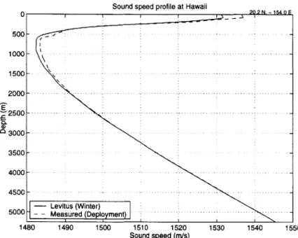
2-1 Sound speed at the ATOC Hawaii array (20.2'N, -154.0'E). The solid line is the profile obtained using temperature and salinity from the Levitus database for the winter season. The dashed line corresponds to the profile computed from a CTD measurement taken at the time of array deployment (mid-November 1995). . . . . 25

2-2 Comparison of Levitus environment and measured environment at Hawaii. The left panel shows a closeup of the sound speed profiles around the channel axis. The right panel shows the modeshapes for the first 10 modes at 75 Hz in each environment . . . . 26 2-3 Modeshapes for the first 10 modes of the Hawaii-Levitus environment

at 60 Hz and 90 Hz. The plot shows the upper 2500 meters of the

(9)

2-4 ATOC environment: geodesic path between source at Pioneer Seamoun-t (off California) and Seamoun-the receiving array near Hawaii. The lefSeamoun-t panel is the average sound speed profile over the path, computed using 235 sections

(~

15 km apart). The right panel shows the differences

be-tween the mean profile and the Levitus (winter) profile for each of the sections. Depth of the ocean bottom, shown in black, is taken from bathymetric surveys of Pioneer Seamount [1] and the ETOPO-5

topography database [2]. . . . . 30 2-5 Sound speed perturbations due to internal waves at 1/2 Garrett-Munk

strength ... ... ... ... 31

2-6 Range-averaged group velocities for the first 40 modes of the CA-HI Levitus environment . . . . 32 2-7 Adiabatic predictions of mode time spread due to dispersion . . . . . 32 2-8 PE simulation through Levitus environment. The top panel is the

received pressure on a 40-element VLA; the bottom panel shows the corresponding arrival time series in the first 10 modes . . . . 33

2-9 PE simulation through Levitus environment plus internal waves . . . 33 2-10 Proposed short-time Fourier mode processing framework . . . . 45

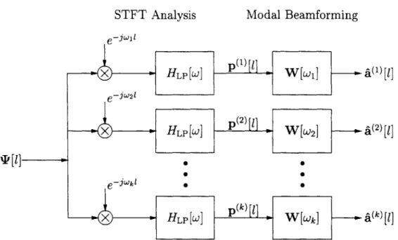
3-1 Block diagram of STFT-based mode processor . . . . 49

3-2 Modeshapes (75 Hz) and receiver locations (+'s) for the design example 59

3-3 MF Beampattern (75 Hz) for the 40-element ATOC VLA in the

Hawaii-Levitus environment . . . . 60

3-4 Comparison of pseudo-inverse filter beampatterns (75 Hz) for the

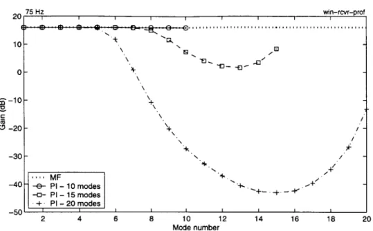
ATOC array in the Hawaii-Levitus environment . . . . 61 3-5 White noise gain at 75 Hz for the ATOC array in the Hawaii-Levitus

environm ent . . . . 62 3-6 M aximum crosstalk . . . . 63

(10)

3-7 Frequency response of the matched filter. Solid lines indicate the

response in the desired mode; dashed lines indicate crosstalk from neighboring modes (up to 10). . . . . 65 3-8 Frequency response of the PI filter designed for 10 modes. Solid

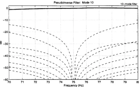
lines indicate the response in the desired mode; dashed lines indicate crosstalk from neighboring modes (up to 10). . . . . 66 3-9 Frequency response of the PI filter for mode 10 (designed using 10

m odes) . . . . 69 3-10 Time and frequency responses for three Hanning windows, assuming

a 300 Hz sample rate. Amplitude differences among the impulse re-sponses are a result of constraining the response to be equal to 1 at 0 H z. . . . . 70 3-11 Simple illustration of time resolution imposed by the lowpass filter . . 71 3-12 White noise gain as a function of frequency for the matched filter and

three different pseudo-inverse filters (for 10 modes, 12 modes, and 15 m odes). . . . . 72 3-13 STFT example: processing of adiabatic propagation data. Top plot

is the received pressure on a 40-element array as a function of time and depth. The bottom plots show the frequency-stacked outputs for modes 1 and 5, respectively. . . . . 74 3-14 Estimated frequency-stacked outputs for the first 10 modes, computed

using a pseudo-inverse filter . . . . 76 3-15 Difference in range-averaged wavenumber and 3-term Taylor series

approximation for the CA-HI Levitus environment. Note that the phase differences are scaled by the range (3515 km) of the ATOC

experiment and normalized by 7r. . . . . 79

3-16 Magnitude and phase across frequency at the peak arrival time in the 75 Hz bin for modes 1 and 5 of the adiabatic example . . . . 82

(11)

3-17 Difference in delay . . . . 86 3-18 Comparison of deployment and recovery sound speed profiles . . . . . 87

3-19 Comparison of deployment and recovery modeshapes at 75 Hz . . . . 88

3-20 Beampattern for the mismatch case: PI filter designed with

deploy-ment profile modeshapes; recovery profile modes are the input . . . . 89

3-21 Beampattern for the mismatch case: matched filter designed with

deployment profile modeshapes; recovery profile modes are the input 89

4-1 ATOC transmission schedule through yearday 509. Crosses mark the

time of each good reception; receptions with bad channels have been eliminated from the data set. The line of numbers below the crosses indicates how the receptions are divided into 13 subgroups for post-processing. . . . . 93

4-2 Estimated noise spectra for hydrophones 10 and 30. The solid line is computed using the noise-only section prior to the signal arrival; dashed line is computed using the noise-only section after the signal arrivals. . . . . 94 4-3 Estimated spatial covariance in the 75 Hz bin; calculated from 300

snapshots. Units are dB, referenced to peak value. . . . . 95

4-4 Input noise levels at 60, 75, and 90 Hz as a function of reception number. 96 4-5 ATOC Reception . . . 100 4-6 PE simulation without internal waves . . . 100 4-7 PE simulation with internal waves at 1/2 Garrett-Munk strength . . 100

4-8 Frequency-stacked mode estimates for the ATOC reception in Fig. 4-5. Color scale is in dB. . . . 101

4-9 Frequency-stacked mode estimates for the PE simulation without in-ternal waves in Fig. 4-6. Black lines in each subplot are the predicted arrival times based on adiabatic dispersion curves. . . . 104

(12)

4-10 Frequency-stacked mode estimates for the PE simulation with internal waves in Fig. 4-7 . . . 105 4-11 Comparison of ATOC data, PE simulations, and adiabatic predictions

for m odes 1 and 10. . . . 106 4-12 Bathymetry near the ATOC source at Pioneer Seamount . . . 107 4-13 Comparison of propagation through the environment that includes the

actual sloping bottom near the source (top plot) and the environment without the slope (bottom plot) . . . 108 4-14 Comparison of arrivals in modes 1 and 10 for the sloping bottom (top

plots) and the zero-slope approximation (bottom plots) . . . 109 4-15 Comparison of the time series for the first 80 modes at 50 km range

from the Pioneer Seamount source. Top plot is for the actual slope. Middle two plots are for the 8.5 degree and 4.3 degree approximations, respectively. The bottom plot corresponds to the no slope case. . . . 110 4-16 Comparison of modes 1 and 10 for the first (top plots) and last (bottom

plots) periods of a source transmission . . . 112 4-17 Comparison of modes 1 and 10 for realizations of a time-varying

in-ternal wave environment. The lag time between the top and bottom plots is 16 m inutes. . . . 113 4-18 Temporal coherence as a function of frequency for mode 1 (left plot)

and as a function of mode number for the 75 Hz bin (right plot). These results were obtained by averaging across 96 receptions (yeardays 363-435). . . . 114 4-19 Variability of modes 1 and 10 across a single transmission (18.2

min-utes) in the 75 Hz bin . . . .. . . . 115 4-20 Variability of modes 1 and 6 for the simulated data in the 75 Hz bin,

calculated at 4 minute intervals. . . . 116 4-21 Mode 1 in ATOC receptions at 4-hour intervals . . . 117

(13)

4-22 Histogram of peak arrivals in the 75 Hz bin. Threshold for peak detection was set at 12 dB above the noise floor. These results were computed from the first 96 good receptions (yeardays 363 to 436). . . 118 4-23 Leading edge, falling edge, and centroid in the 75 Hz bin for the first

20 ATOC receptions, each consisting of 10 four-period averages. . . . 119 4-24 Comparison of average leading and falling edges for the first group of

ATOC receptions and the simulated data set . . . 120

4-25 Comparison of average centroid locations for the first group of ATOC receptions, the simulated receptions, and adiabatic predictions . . . . 122 4-26 Average centroids as a function of frequency for the first 7 groups of

ATOC receptions. Legend is identical to that shown in Fig. 4-25. See

Fig. 4-1 for a definition of the groups. . . . 124 4-27 Average centroids as a function of frequency for groups 8-13 of the

ATOC receptions. Legend is identical to that shown in Fig. 4-25. See

Fig. 4-1 for a definition of the groups. . . . 125 4-28 Average centroids in the 75 Hz bin for modes 1-10 as a function of

yearday . . . .. . . 126 4-29 Average leading and falling edges for mode 1 in the 75 Hz bin as a

function of yearday . . . 127 4-30 Average of the RMS error over 13 groups of receptions as a function

of mode number. Results are shown for the centroids and the falling edges of the 75 Hz bin. . . . 128

(14)

Chapter 1 Introduction

Normal modes provide a convenient description of low-frequency sound in the deep ocean. Their strong connection to the propagation environment makes them useful in a variety of applications, including source localization and acoustic tomography. Currently, there is much interest in using modes to analyze broadband receptions at megameter ranges for the purpose of studying ocean variability on basin-scales. At these ranges, the effects of internal waves on mode coherence are not known. This thesis develops a signal processing framework for estimating modal time series and uses it for analyzing data from the Acoustic Thermometry of Ocean Climate experiment. From a signal processing perspective, the key issue to consider is the broadband nature of the signals; specifically, any approach must accommodate vari-ations in the mode characteristics across the bandwidth of the source. In examining the data, the focus is on understanding the fluctuations of mode arrivals and char-acterizing the complicated multipath structure.

The rest of this chapter introduces the research questions addressed by this thesis. As a starting point, the following section motivates the use of the modal description in the context of long-range acoustics and discusses open questions about megameter propagation. The second section highlights some of the signal processing issues surrounding the broadband mode estimation problem. Section 1.3 describes the

(15)

Avg. Speed 0 r Source / Rcvr 1000 Array 2 2000 a 3000-4000 5000 1500 1550 0 500 1000 1500 2000 2500 3000 3500 Range (km)

Figure 1-1: Deep ocean waveguide. The left panel shows a typical deep water sound speed profile. The right panel illustrates how refractive effects permit propagation over extremely long ranges.

opportunities presented by the recent ATOC experiment. Finally, Section 1.4 states

the specific research objectives and outlines the remainder of the thesis.

1.1 Use of Modes in Long-Range Acoustics

The deep ocean is an efficient channel because it traps low-frequency acoustic signals, enabling them to be detected thousands of kilometers from their source. Figure 1-1

shows how the refractive effects of the underwater waveguide allows propagation to

such long ranges. Acoustically, the deep ocean is characterized by a sound speed

profile with a minimum, between 800 and 1200 meters depth, known as the sound

channel axis. Sound waves bend towards regions of lower velocity, thus the minimum

creates a duct. As the figure depicts, a sound wave leaving the source on a downward

trajectory bends back towards the axis. Once it passes through the minimum on an

upward path, it bends away from the surface. Purely refracted paths, such as the

one shown, do not scatter energy at boundary interactions. Since absorption losses for low frequencies (on the order of 100 Hz) are minimal, the signals can propagate

(16)

Received pressure 364084024.cirlO.hva ₀ 400 600 _-5 800 51000 -10 1200 1400 -15 1600 -20 2368 2369 2370 2371 2372 2373 2374 2375 2376 Time (seconds)

Figure 1-2: Broadband reception on 40-element VLA located 3515 km from source

over extremely long distances in the channel.

Fig. 1-2 illustrates some general features of pulse propagation to megameter ranges. The plot shows the pulse-compressed and sequence-averaged time series recorded by a 40-element vertical line array (VLA) located 3515 km from a broad-band source. Inter-element spacing is 35 m, and the array is approximately centered on the sound channel axis. This figure reveals an important characteristic of propa-gation in the underwater sound channel, namely the time-spread of the arrivals due to the fact that they take many different paths between source and receiver. The early arrivals traverse deep-diving ray paths that are associated with higher group ve-locities because they sample the water away from the sound speed minimum. Signals that propagate almost horizontally, along the sound channel axis, arrive last and are often more energetic. In general, the multipath arrival structure can be represented in terms of the vertical eigenfunctions, or normal modes, of the underwater wave-guide. Modal dispersion accounts for the time-spread of the signal at long ranges. In deep water, the high modes travel faster than the low modes, thus the high modes are associated with the early-arriving energy in Fig. 1-2. The planewave-type arrivals visible in the early parts of the reception (up until ~ 2373 seconds) are the result

(17)

not evident in the last 2.5 seconds of the reception, associated with the low mode arrivals.

As solutions to the frequency-dependent wave equation, the modes provide many useful insights about sound propagation. Each mode essentially samples a different

part of the water column: the low modes are concentrated around the axis, whereas the higher modes have greater vertical extents. Since the modes depend strongly on the environment, they can be used as observables for matched field processing or tomography applications. The key to matched field or tomographic inversions is the ability to associate an arrival with a particular path or section of the water column. In range-invariant environments, this problem is trivial because the modes propagate independently without exchanging energy, i.e., an arrival in mode 1 is known to have traversed the entire path in mode 1. For a realistic ocean environment, however, inhomogeneities cause coupling of energy among the modes, which makes the problem much more difficult. Understanding the mechanisms and effects of mode coupling is crucial to using these signals in any type of application.

At long ranges, internal waves are thought to be the primary source of coupling. Vertical displacements of water associated with internal waves cause fluctuations of the temperature, thus changes in the sound speed, at a fixed depth. The horizontal variability of these sound speed fluctuations, in turn, can cause an exchange of en-ergy among the modes as they propagate. The effects of these fluctuations on the planewave-type arrivals are fairly well-understood - these arrivals are amenable to analysis via geometrical optics approximation. Significantly less is known about the axial mode arrivals since there is no comparable theory. The late-arriving modes tend to describe the most energetic, trapped signals and thus are useful in detect-ing/estimating weak sources at long range. To develop an understanding of how these low modes propagate through internal wave fields and to test some of the limited theoretical results, it is necessary to study them experimentally.

(18)

1.2 Broadband Mode Estimation at Megameter

Ranges

Measuring the mode arrival structure at long ranges presents an interesting signal processing problem. Unlike the planewave arrivals, axial mode arrivals generally overlap in time, and must be estimated via spatial processing. Since the modes are an orthonormal basis in depth, in principle they can be separated using vertical line arrays spanning the entire water column. In practice, the degree of orthogonality of the modeshapes, as sampled by a practical array, determines how well the modes can be resolved.

A key issue in this thesis is the use of broadband signals. The modes are

inher-ently frequency-dependent, since they are derived from the frequency-domain wave equation. Previous work on mode estimation has primarily focused on situation-s where a narrowband approximation isituation-s valid, i.e., either the situation-source isituation-s CW or the mode functions are approximately constant across the band of the source. A few researchers have implemented broadband mode processors using an FFT for the fre-quency decomposition, but they have not discussed the frefre-quency resolution required for this approach. What is needed is a general framework for broadband mode esti-mation that will allow a careful analysis of performance in terms of mode resolution

and time/frequency resolution.

A recent experiment provides an opportunity to develop methods of mode

pro-cessing and to apply them to studying the coherence of mode arrivals at megameter ranges.

(19)

ATOC source and receiver locations I QQ~1 QQ~~ 60N 5ON 40N - Pioneer Seamount 30N - 3515 km 20N - 5171 km-Hawaii 10N -0 Kiritimati (Christmas Island) 180W 160W 140W 120W 100W 80W 60W Longitude

Figure 1-3: ATOC source and receivers

1.3 Acoustic Thermometry of Ocean Climate

Experiment

The purpose of the Acoustic Thermometry of Ocean Climate (ATOC) experiment is to study long-range propagation of sound and to investigate acoustic methods for monitoring ocean climate variability. The intent is to demonstrate that travel-time tomography can be used to measure ocean temperature over ranges of 3,000 to

10,000 km. The ATOC network consists of a broadband source off the California

coast, two vertical line arrays, and a number of bottom-mounted horizontal arrays. This thesis focuses on analyzing data from the two VLA's, which were designed to spatially resolve the lowest 10 modes at each location. Figure 1-3 shows the location of source and receivers considered in this thesis. The path lengths to the receivers at Hawaii and Kiritimati (Christmas Island) are 3515 km and 5171 km, respectively.

(20)

These arrays were deployed in November 1995 and recovered in September of 1996. The bottom-mounted source (934 m) on Pioneer Seamount transmitted pulses at a center frequency of 75 Hz. Each transmission consists of 40 periods of a pseudo-random sequence, phase modulated onto a 75 Hz carrier. The receiver averages every 4-periods internally. Over the duration of the experiment, transmissions are sent every 4 hours during periods established by the ATOC Marine Mammal Research

Program.

ATOC presents the first opportunity to study mode arrivals at megameter ranges.

The next section outlines the objectives of this thesis.

1.4 Thesis Objectives

The first objective of this research is to define a framework for broadband mode estimation. Since the modeshapes are frequency-dependent and the mode spectral coefficients are time-dependent, mode estimation involves a combination of temporal and spatial filtering. Most previous work has focused primarily on the narrowband mode estimation problem, and has not addressed issues unique to broadband signals. The second objective is to analyze the low-order mode arrivals in the ATOC data. This is really the first opportunity of its kind. Specifically, this research hopes to

characterize the complicated mode arrival structure and explore the effects of internal waves on mode coherence.

The organization of the thesis is as follows. Chapter 2 reviews background about normal mode representations and motivates several specific questions about long-range mode propagation. It clearly formulates the broadband mode estimation problem and proposes and approach for exploring the scientific/signal processing research topics using the ATOC data. Following that, Chapter 3 presents a frame-work for broadband mode processing, based on short-time Fourier techniques. The fourth chapter presents an analysis of the ATOC data set for the Hawaii array,

(21)

compares these results to simulations, and identifies several useful statistics of the mode arrivals. Finally, Chapter 5 summarizes the thesis contributions and indicates directions for future research.

(22)

Chapter 2 Background

As indicated in Chapter 1, normal modes are of interest in applications such as tomography and thermometry because the lowest modes provide a convenient de-scription of the energetic late arrivals at megameter ranges. This chapter lays the groundwork for the rest of the thesis by motivating specific questions about long-range mode propagation, clearly formulating the broadband mode estimation prob-lem, and proposing an approach for exploring these research topics using data from the ATOC vertical arrays. The material is divided into four parts. Section 2.1 re-views the salient characteristics of the normal mode representation and outlines some of the open questions concerning mode propagation through range-dependent and random environments. In the course of describing relevant features of the modal basis set, this section also introduces a range-dependent ocean environment, which is used for many of the examples in later chapters. Given this mathematical back-ground and experimental motivation, Section 2.2 poses the mode estimation problem for vertical arrays and highlights important design considerations. In particular, the discussion emphasizes the broadband character of the problem since most prior work has focused on using modes to analyze narrowband signals. The third section reviews previous work on mode estimation in order to place the current research in context. Finally, Section 2.4 outlines the proposed approach, which is based on short-time

(23)

Fourier analysis techniques, and describes the areas addressed by the rest of the thesis.

2.1 Broadband Normal Mode Representation

Normal mode representations are useful in describing the acoustic pressure field in a variety of underwater environments. Several standard textbooks develop acoustic mode theory in detail [3, 4, 5]. The following discussion reviews the basic concepts, focusing primarily on modal representations for broadband signals in deep ocean environments such as those encountered in ATOC. This section is split into two parts: the first describes the use of the modes as a "local" basis set for the pressure field; the second discusses mode propagation in a variety of environments.

2.1.1 "Local" Orthonormal Basis

Normal modes are the eigenfunctions of the ocean waveguide, which are derived from the frequency domain wave equation (Helmholtz equation). At each frequency, a mode is characterized by its wavenumber km and its modeshape 0m. For a given environment, defined by the sound speed profile and boundary conditions, the modes satisfy a second-order eigenvalue equation, e.g., in cylindrical coordinates (assuming constant density):

d24 (r, Z, Q) +

[k2(r, z,

Q) - km(r, Q)] Om(r, z, Q) = 0; _{k(r, z,}_Q)

dz2 M c(r, z)

(2.1) In Eq. 2.1, Q is the temporal frequency, c(r, z) is the sound speed as a function of range r and depth z, and k(r, z, Q) is the medium wavenumber. The modal wavenumber (km) determines propagation characteristics, such as phase and group speeds, and the modeshape determines the spatial distribution of pressure due to

(24)

each mode. These shapes are orthogonal functions, scaled such that

1 jZax Om(Q, z)4,(Q, _z)dz₌_6(m

-n), _(2.2)

p 0

where p is the density of water.

Since the modes are an orthonormal basis for narrowband signals, the pressure field at coordinates (r, z) can be represented as the weighted sum

p(r, z, )= am(r, Q)Om(r, z, £) (2.3)

m

where am is the frequency-dependent coefficient for mode m. In general, the sum in Eq. 2.3 is infinite, although in most realistic environments only a finite number of modes contribute significantly to the field. The remaining "leaky" modes have complex wavenumbers and suffer exponential losses as they propagate, thus their contributions are negligible in the far-field of the source. This thesis focuses on long-range propagation scenarios where it is reasonable to represent the pressure field with a finite set of modes.

Time- and frequency-domain representations of the pressure are related via Fouri-er synthesis, i.e., the time sFouri-eries for a receivFouri-er at range r and depth z is

(r, z, t) = 1f r, z, Q)e'dQ = 1 am(r, £)4m(r, z, ) ejntdQ. (2.4)

Similarly, the inverse Fourier transform of the frequency-dependent mode coefficient

am(£) in Eq. 2.3 defines the time series associated with mode m at range r:

am(r, t) = - fam(r, Q)ejftd. (2.5)

27r Q

Limits of integration in the above equations are determined by the source bandwidth and the frequency range over which the relevant modes are propagating.

(25)

nor-Sound speed profile at Hawaii 2 ? N - 154-0 E 500 -- - - - - -- -- ---1000 - - - --- - - --1500 - ---- - --- ----0 o 3000 - - - --- - -- 3500- 4000- 4500-- Levitus (Winter) 5000 - - _{Measured (Deployment)} 1480 1490 1500 1510 1520 1530 1540 1550 Sound speed (m/s)

Figure 2-1: Sound speed at the ATOC Hawaii array (20.2'N, -154.0'E). The solid line is the profile obtained using temperature and salinity from the Levitus database for the winter season. The dashed line corresponds to the profile computed from a

CTD measurement taken at the time of array deployment (mid-November 1995).

mal modes using the environment at the ATOC Hawaii array. Figure 2-1 shows the sound speed profile for this location, computed from Levitus climatological da-ta [6, 7]. For reference, the plot also includes the profile derived from environmenda-tal measurements taken during the array deployment. Figure 2-2 shows the first 10 modeshapes at 75 Hz for both of these environments.' Note that each mode samples a different part of the waveguide: the lowest modes are concentrated around the sound channel axis, while the higher order modes cover greater extents of the water column. The modes of these two environments are qualitatively similar, however the shapes do reflect the differences in sound speed (up to 1 m/s near the channel axis).

Since the medium wavenumber depends on frequency as well as sound speed, the modes are functions of frequency, in general. To demonstrate this, Figure

2-3 compares the modeshapes at 60 and 90 Hz for the Levitus environment. The

(26)

Environmental dependence of modeshapes: Levitus vs. measured 200 1 NZ 400-600 - - - -8 0 0 -/--/ 1000 - --- ) -E _ 1 2 0 0 -- -- 1400---1600 -N -1800 - -2000- - - Levitus (Winter) - - Measured (Deployment) 2200 ' 1482 1486 14900 1 2 3 4 5 6 7 8 9 10 11

Speed (m/s) Mode number

Figure 2-2: Comparison of Levitus environment and measured environment at Hawai-i. The left panel shows a closeup of the sound speed profiles around the channel axis. The right panel shows the modeshapes for the first 10 modes at 75 Hz in each envi-ronment.

frequency range on the plot corresponds to the approximate bandwidth of the ATOC source. Over this 30 Hz interval, mode 1 varies slightly, whereas mode 10 changes quite significantly. In general, the environment and the source bandwidth determine the extent of modal.frequency dependence. As this example clearly shows, modal frequency variations are an important factor to consider in the ATOC experiment.

The formulation in Equations 2.1-2.5 emphasizes that the modes are an orthonor-mal basis for a particular environment, defined by c(r, z). Based on their spatial distributions, the lowest modes (eigenfunctions) can provide a compact description of acoustic energy concentrated around the sound channel axis. Beyond being useful as a "local" basis set, the modes are interesting because they are strongly connected with the propagation of signals in the ocean waveguide. The following section dis-cusses how modes propagate in a variety of different environments and raises some questions about long-range sound transmissions.

(27)

Modeshapes at Hawaii (Levitus profile) n , \ I 500 - 7 g 1000-S/ E 2000.--- 60 Hz S90Hz 21500 1 M 3 20t 1 2 3 4 5 6 7 8 9 10 11 Mode number

Figure 2-3: Modeshapes for the first 10 modes of the Hawaii-Levitus environment at 60 Hz and 90 Hz. The plot shows the upper 2500 meters of the 5250 meter waveguide.

2.1.2 Mode Propagation

From a simple input/output viewpoint, the underwater channel transforms the mode

signals excited by the source into a modal time series at the receiver. Assuming a finite number of propagating modes, a concise frequency-domain description of this

system is

a[r, Q] = T[Q]a[0, Q] (2.6)

where a[0, Q] is a vector of mode amplitudes at the source (r = 0) and a[r, Q] represents the corresponding vector at the receiver. For a point source, the modes are excited at levels proportional to the source spectrum Srrc and the amplitude of

the modeshape at the source depth z, i.e.,

a[0, Q] = Ssc[]0,( ,z )(2.7)

(28)

In Eq. 2.6, T[Q] is a square matrix that defines the transformation of the spectral amplitudes, according to how the modes propagate in the channel. There are two broad classes of propagation environments to consider: independent and range-dependent.

Range-Independent Environments

Given a fixed sound speed profile and bottom depth, the modeshapes and wavenum-bers are independent of range. In this case, the modes propagate without exchanging energy, i.e., T is a diagonal matrix:2

0

TRI[Q] = __ eikmr (2.8)

0

In this type of waveguide, each mode is a standing wave in depth that propagates outward from the source with a group velocity equal to dQ/dkm. In general, group velocity varies with mode number and frequency, meaning that the channel is dis-persive. For a deep water environment, the low modes travel slowest, since they represent energy trapped around the sound speed minimum; higher modes travel faster. In a deep channel, modal group velocity typically decreases with frequency.

Range-Dependent Environments

For realistic ocean waveguides, the environment is a function of range, or more gen-erally, a function of range and azimuth. When the medium is inhomogeneous due to variations in sound speed and/or bathymetry, the modes no longer propagate inde-pendently. Instead there is coupling of energy among the modes, meaning that the T matrix has non-zero off-diagonal terms. A range-dependent waveguide can be

mod-2_{Eq. 2.8 assumes the receiver is in the farfield of the source. See [4, 5] for a discussion of}

(29)

eled using a cascade of range-independent segments. In this type of model, boundary conditions at the segment interfaces determine the mode coupling coefficients.

Since the coupled-mode approach leads to a computationally-intensive implemen-tation, it is useful to consider a simplification. The adiabatic approximation assumes the range dependence is weak and neglects the coupling terms, reducing T to a di-agonal matrix. Under this assumption, each propagating mode adapts with range (changes shape and wavenumber), but does not transfer energy into the other modes. For an adiabatic model the range-averaged wavenumber,

km =- km(r')dr', (2.9)

r 0

determines the phase and group speeds for mode m, thus the adiabatic propagation matrix, TAD, is simply TRI with km replaced by km. Obviously the validity of the adiabatic assumption is related to the nature of the inhomogeneities in the medium. Desaubies has analyzed this problem in detail, concluding that the approximation's accuracy depends strongly on frequency, mode number, range and the acoustic quan-tity of interest, e.g., intensity, phase travel time [9, 10].

In long-range experiments, there are several types of inhomogeneities that may cause mode coupling. Consider the environment along the geodesic connecting ATOC source at Pioneer Seamount to the receiving array at Hawaii, shown in Fig. 2-4. The plot shows how the Levitus (winter) sound speed profiles change over the 3515 km path. Variability is concentrated in the upper 500 m of the water column and is a relatively mild function of range. The figure also displays the bathymetry for this section of the ocean. In a deep water environment, changes in the bottom are unlikely to affect the axial modes since they do not interact with the waveguide boundaries. For these modes, the most significant feature of this path is the rapid dropoff in the vicinity of Pioneer Seamount. The bottom-mounted source (935.5 m) does not directly excite the lowest modes. Instead they are excited by energy that couples from the higher order modes as the sound propagates downslope. Chapter 4 explores

(30)

Avg. SSP Difference from mean profile 0 15 10 'a 1000 5 2000 0 EW _-5 CL 3000 --10 CL 4000 -15 u C §000 -20 5000--25 1480 1555 0 500 1000 1500 2000 2500 3000 3500 Cavg(z) Range (km)

Figure 2-4: ATOC environment: geodesic path between source at Pioneer Seamount (off California) and the receiving array near Hawaii. The left panel is the average sound speed profile over the path, computed using 235 sections

(~

15 km apart). The right panel shows the differences between the mean profile and the Levitus (winter) profile for each of the sections. Depth of the ocean bottom, shown in black, is taken from bathymetric surveys of Pioneer Seamount

[1]

and the ETOPO-5 topography database [2].

the issue of bathymetric coupling and its implications for the mode arrivals measured in ATOC.

As indicated in Chapter 1, internal waves are expected to be the primary source of mode coupling in long-range propagation experiments. In the deep ocean, in-ternal wave variability is typically modeled using the empirical Garrett-Munk spec-trum [11, 12]. Figure 2-5 shows one realization of sound speed perturbations due to internal wave fluctuations, computed using the method of Colosi and Brown [13]. The calculation assumes the internal waves are 1/2 Garrett-Munk strength. Note that the variability is greatest in upper part of water column.

Before reviewing what is known about mode propagation through random internal

wave fields, it is useful to consider two simulation examples. The first shows how broadband signals propagate through the slowly-range-varying Levitus environment. As a comparison, the second example illustrates the effects of internal waves by adding the sound speed perturbations of Fig. 2-5 to the background environment.

(31)

Internal wave sound speed perturbations - single realization 0 4 3 2002 400 C 600 -1 3 -2 800 -3 1000 -4 0 500 1000 1500 2000 2500 3000 3500 Range (km)

Figure 2-5: Sound speed perturbations due to internal waves at 1/2 Garrett-Munk strength

For simplicity, both simulations use an axial (rather than bottom-mounted) source and ignore the seamount.

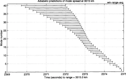
To develop some general intuition about propagation in the unperturbed Levitus environment, consider the adiabatic group velocities. Figure Figure 2-6 shows the ve-locities for the first 40 modes, derived from the average wavenumbers for the 3515 km path. On the plot, the bottom line on the plot corresponds to mode 1 and the top line corresponds to mode 40. Group velocity decreases with frequency and increases as a function of mode number, as is typical in a deep water channel. Figure 2-7 shows the predicted spread of mode arrival times at 3515 km range, assuming a bandlimited source spectrum between 60 and 90 Hz and adiabatic propagation. As expected from the group velocity curves, the high modes arrive first and exhibit the most dispersion, while the low modes arrive last and are less spread. Mode 1 is undispersed since its group speed is approximately constant with respect to frequency.

Figure 2-8 shows the results of a broadband parabolic equation (PE) simulation

through the Levitus background environment. The top plot is the pressure time series at the Hawaii array location, calculated using the RAM PE code [14].' Individual

3

(32)

-- ~

Range-averaged group velocity: CA-HI path

1483.5 1483- 1482.5--E 148 2 Z. ... 0 1481 1480.5-1480 60 65 70 75 80 85 90 Frequency (Hz)

Figure 2-6: Range-averaged group velocities for the first 40 modes of the CA-HI Levitus environment

Adiabatic predictions of mode spread at 3515 km win-range-avg

40 ... . 35 -_-_-_-_ _-_- -. 30... . ... ... 35 -~25 E -20 15 - -. . 10 . 5 - . - -. --HH 01 2369 2370 2371 2372 2373 2374 2375

Time (seconds) to range = 3515.0 km

(33)

400 600 800 0) E 1000 1200 1400 1600 20 - 15 C 10 05 2372 2372.5 2373 2373.5 2374 2374.5 Time (seconds)

Figure 2-8: PE simulation through Levitus environment. ceived pressure on a 40-element VLA; the bottom panel arrival time series in the first 10 modes

400 600 800 WI) E 1000 -C 1200 1400 1600 20 E15 C 10 05 2372 2372.5 2373 2373.5 2374 2374.5 Time (seconds) 0 -5 -10 -15 -20 -25 -10 -20 2375

The top panel is the re-shows the corresponding

0 -5 -10 -15 -20 -25 -10 -20 2375

(34)

mode arrivals are evident in the pressure field, e.g., modes 5, 3, 1. Below the pressure plot is the modal time series obtained by projecting the PE field onto the functions at the receiver. The modes are obviously arriving in order from highest to lowest. The constructive interference of the higher modes result in the planewave (ray) arrivals in the early part of the reception.4 _{Each of the low modes appears to have a single}

dominant peak, which arrives at the predicted adiabatic arrival time. This implies that that the range variations in the sound speed do not result in mode coupling. Dispersion characteristics of the waveguide are evident.

In contrast, Fig. 2-9 shows the analogous results of the PE simulation for the Levitus environment plus internal waves. The picture is quite different. Individual modes are no longer visible in the pressure time series. From the mode time series, it appears that instead of a single, dispersive arrival in each mode, there are multiple arrivals. This "modal multipath" creates the complicated interference patterns seen in the pressure waveforms. Comparing these two examples to the ATOC reception shown in Fig. 1-2 of Chapter 1 reveals that the experimental measurement more

closely resembles the internal wave simulation.

From a theoretical standpoint, the effects of internal waves on long-range sound propagation are not fully understood. Most previous work has focused on the ray arrivals because they are amenable to analysis via the geometric optics approxima-tion. The monograph by Flatte et al. summarizes the path integral theory that predicts the fluctuations and coherence of resolved rays [17]. No corresponding the-ory exists for predicting the behavior of the mode arrivals. The following discussion reviews important results regarding mode propagation through internal waves (but does not attempt a comprehensive overview of work in this area).

In two seminal papers, Dozier and Tappert derive statistics for the modal in-tensities of narrowband signals propagating in a random ocean [18, 19]. Based on theoretical work and a set of numerical simulations, they conclude that scattering

(35)

eventually results in an equipartition of energy among the modes. To make the problem tractable, the authors rely on a number of key assumptions, which may not be valid in real ocean environments. Notably they assume that the acoustic modes are mutually incoherent (phase-random) and that there is no loss of energy into the bottom. Regarding the first assumption, Nechaev has shown that partial coherence of the modes can prevent the equipartition of energy predicted by Dozier and Tap-pert [20, 21]. Nechaev's analytical results indicate that decorrelation of neighboring modes can occur more slowly than the randomization of the overall field and that scattered modal energy can form a stable interference structure.

A series of papers in the Russian literature have investigated the degradation of

mode coherence by internal waves and the resulting implications for various sig-nal processing methods, e.g., matched filtering [22], horizontal array beamform-ing [23, 24], and vertical array beamformbeamform-ing [25]. Recently, Sazontov has developed an approximate analytic method for computing the modal cross-coherences and using them to calculate the mutual coherence function for the total field [26]. Gorodet-skaya et al. provide an excellent introduction to this technique, applying it to a study of horizontal and vertical array gain limitations due to internal wave fluctu-ations [27]. At present, it is not known how well the approximate expressions for coherence agree with experimental data.

Prior to ATOC, there have been very few opportunities to observe the axial arrivals at megameter ranges. Researchers have relied heavily on numerical simula-tions to test theories about the late-arriving mode energy. In one of the first looks at experimental data, Colosi et al. compare pressure measurements from the 1000 km SLICE89 experiment to broadband PE simulations [28]. Their results show that the broadening of the transmission finale in the data is attributable to internal waves. This smearing in depth of the final axial arrivals is due to an exchange of energy a-mong the modes. Colosi and Flatte explore the subject of mode coupling via internal waves using PE simulations designed to model certain aspects of the ATOC

(36)

experi-ment [29]. They show that mode propagation through these random fields is strongly non-adiabatic and quantify the travel-time bias/spread and intensity fluctuations for the modes. According to Colosi et al.'s recent review article, internal-wave-induced mode coupling, while definitely an issue at 75 Hz, may be significantly reduced at lower frequencies, e.g., 28 Hz [30].

Internal waves can obviously limit the effectiveness of tomographic inversions or MFP applications since it hampers the ability to associate an arrival with a particular path through the ocean. As indicated by this overview, there is much left to learn about broadband mode propagation through internal wave fields. Characterizing the mode arrival structure is a prerequisite to using the modes in tomography or source localization. The ATOC experiment is the first to have mode-resolving arrays deployed to measure axial modes at megameter ranges over a period of months. The following section describes some specific questions that this thesis proposes to explore using the ATOC receptions.

Questions About Long-Range Mode Propagation

This thesis seeks to address the following questions concerning long-range mode propagation. By answering these questions we hope to gain insight into how to identify appropriate observables for tomography and other applications.

First, a general question about axial arrivals at megameter ranges:

" How to characterize the mode arrival structure?

- is each mode dominated by a single, dispersive arrival?

- is there multipath?

- are the dispersion characteristics of the channel evident? * How do the mode signals vary with time?

The next question requires a different approach than previous researchers have taken, namely it requires short-time frequency decompositions.

(37)

" Can the characteristics of individual multipaths within a mode be measured?

How do they compare with the ray arrivals?

- temporal coherence?

- frequency coherence? resolvable multipath?

- fluctuation statistics

" How does the downslope propagation/bottom interaction near the source affect

the initial mode excitations. In turn, how does that affect the receptions at megameter ranges?

For an experiment like ATOC where there are many questions about the forward propagation, it is crucial to design a mode estimator that doesn't assume any a

priori knowledge of the arrival structure and to thoroughly analyze the estimator's

behavior. The following section defines the broadband mode estimation problem and identifies the various factors that determine mode resolution.

2.2 Broadband Mode Estimation Problem

In general, the low order modes are not temporally resolvable [31], meaning that they are not directly observable in the time series from a single hydrophone. In-stead, vertical arrays can be used to separate the mode signals based on their spatial characteristics. This approach relies heavily on the orthogonality of the sampled modes.

Using Eq. 2.3, the noisy pressure field at frequency Q, sampled by an N-element vertical array, may be written:

A

pr, Zi

7Q)

1 (r, zi,Q) ...

Om

a,(,Q

1r

[i)

n(zl, Q)1

p(r, zN, )[ 1(r, zN, Q) ... M(r, zN, Q) aM (r,1) n(ZN,

J

(38)

or in vector notation:

p[r, Q] = 4[r, Q]a[r, Q] + n[Q]. (2.11)

4 is the matrix of sampled modeshapes, a is the vector of mode amplitudes, and n

is the vector of observation noise. Eq. 2.10 assumes that the signal consists of M

propagating modes. In the case of a broadband source, the array actually measures

a vector time series, i.e., from Eq. 2.4,

xI(r, t) = p[r, Q]ejtdQ = (4[r, Q]a[r, Q] + n[Q]) edtdQ. (2.12)

This thesis considers the problem of estimating the mode signals (i.e., a[Q]) from

noisy measurements of the pressure field. A number of important signal processing

is-sues arise in designing broadband mode estimators. The rest of this section discusses

these issues in detail, using the ATOC experiment as the motivating example.

Modal frequency dependence is the most important issue to consider in broadband

mode estimation. As Fig. 2-3 demonstrates, modeshapes can vary significantly across

a 30 Hz source band. Clearly, spatial processing must be done on a set of subbands

to avoid mismatch problems. Since a combination of temporal and spatial filtering

is required, there are time/frequency tradeoffs to make. Good time resolution is

desirable for resolving the individual multipaths within a mode. The allowable widths

of the subbands is determined by the environment, i.e., the modeshape variations.

On a band-by-band basis, mode estimation reduces to a classic linear inverse

problem, discussed in many areas of the literature, e.g., estimation theory [32],

geo-physical inverse theory [33]. In the narrowband mode estimation problem, the key

issue to consider is the degrees of freedom of the sampled modeshape matrix. This

de-termines how well the processor can resolve a mode and reject noise. From the point

of view of estimating one mode, there are two types of noise to consider. The first

component consists of signals propagating in the other modes - this is structured in-terference and may be correlated with this signal. The second is measurement noise

(39)

that uncorrelated with the signal, e.g., shipping noise, sensor noise. Note that in terms of interference rejection, we assume that some time windowing can be done to limit the number of modes contained in the measurement, i.e., the ray arrivals (high order modes) can be ignored by time-gating.

In addition to time/frequency tradeoffs and degrees of freedom concerns, two other issues arise in implementing mode estimators for realistic experiments. The first concerns arrays that are not perfectly vertical. This can be modeled by using a complex modeshape matrix - the phase terms represent the timing corrections required for each mode. In planewave beamforming, this is known as the array transit time problem. It is important to quantify the limitations it places on the processor for modes. Usually, reliable mooring motion estimates are available, so the problem is one of correcting for known delays.

A second practical concern relates to the dependence of the mode on the local

environment at the array. Mode environmental dependence is the key to using them in tomography or matched field processing, but can be a hindrance when the receiver environment is not exactly known. Uncertainty in our knowledge of <>[Q] affects ability to resolve the mode signals accurately. Consider the measured and archival profiles shown in Fig. 2-2. In this case, the archival profile does not adequately represent the modes of the measured environment. In ATOC the problem is that we only have two measurements of the environment: one at deployment and one at recovery. The time lapse between those two is approximately 9 months. It is expected that mesoscale effects and seasonal changes affect the profile over the course of the experiment, so that there may be mismatch between the modes of the measured profile and the true profile. It is important to quantify the effects of mismatch on mode processing.

In summary, there are a number of important design considerations in broadband mode estimation. The following section reviews relevant literature on mode filter-ing techniques and their application to tomography, focusfilter-ing in particular on how