Bias corrected instrumental variables estimation for dynamic panel models with fixed effects

Digitized

by

the

Internet

Archive

in

2011

with

funding

from

Boston

Library

Consortium

IVIember

Libraries

Massachusetts

Institute

of

Technology

Department

of

Economics

Working

Paper

Series

BIAS

CORRECTED

INSTRUMENTAL

VARIABLES ESTIMATION

FOR

DYNAMIC

PANEL

MODELS

WITH

FIXED EFFECTS

Jinyong

Hahn

Jerry

Hausman

Guido

Kuersteiner

Working

Paper

01

-24

June

2001

Room

E52-251

50

Memorial

Drive

Cambridge,

MA

02142

This

paper

can

be

downloaded

without

charge

from

the

Social

Science

Research Network

Paper

Collection

at

MASSACHUSEHS

INSTITUTE

OFTECHNOLOGY

Massachusetts

Institute

of

Technology

Department

of

Economics

Working

Paper

Series

BIAS

CORRECTED

INSTRUMENTAL

VARIABLES

ESTIMATION

FOR

DYNAMIC

PANEL

MODELS

WITH

FIXED

EFFECTS

Jinyong

Hahn

Jerry

Hausman

Guide

Kuersteiner

Working

Paper

01

-24

June

2001

Room

E52-251

50

Memorial

Drive

Cambridge,

MA

021

42

This

paper

can be downloaded

without

charge

from

the

Social

Science

Research Network

Paper

Collection

at

Bias

Corrected

Instrumental Variables

Estimation

for

Dynamic

Panel

Models

with Fixed

Effects

Jinyong

Hahn

Jerry

Hausman

Guido

Kuersteiner

Brown

University

MIT

_MIT

June,

2001

Acknowledgment:

We

are grateful to

Yu

Hu

for exceptional research assistance. Helpful

comments

by

Guido

Imbens,

Whitney

Newey,

James

Powell,

and

participants of

workshops

at

Arizona

State University, Berkeley

Harvard/MIT,

Maryland,

Triangle,

UCL,

UCLA,

UCSD

are appreciated.

Abstract

This

paper

analyzes the second order bias of instrumental variables estimators for a

dynamic

panel

model

with fixed effects.

Three

different

methods

of second order bias correction are

considered. Simulation experiments

show

that these

methods

perform

well if the

model

does

not

have

a root near unity but

break

down

near the unit circle.

To remedy

the

problem

near the unit root a

weak

instrument

approximation

is used.

We

show

that

an

estimator

based

on

long differencing the

model

is

approximately

achieving the

minimal

bias in

a

certain class of

instrumental variables (IV) estimators. Simulation experiments

document

the

performance

of the

proposed

procedure in finite samples.

Keywords:

dynamic

panel, bias correction,

second

order, unit root,

weak

instrument

reduces the finite

sample

bias

and

alsodecreases the

MSE

ofthe estimator.

To

increeise further the explanatory

power

ofthe instruments,

we

use the technique ofusing estimated residuals as

additional instruments a technique introducedinthesimultaneous equations

model by Hausman,

Newey, and

Taylor (1987)

and

used in the

dynamic

panel

data

context

by

Ahn

and Schmidt

(1995).

Monte

Carloresults

demonstrate

that the long differenceestimator

performs

quite well,

even for high positive values of the lagged variable coefficient

where

previous estimators are

badly biased.

However,

thesecond orderbiascalculations

do

notpredict wellthe

performance

ofthe

estima-tor for these high values ofthe coefficient. Simulation evidence

shows

that our

approximations

do

not

work

well near the unit circle

where

the

model

suffers

from

a near non-identification

problem. In order to analyze the bias of

standard

GMM

procedures

under

these circumstances

we

consider alocal to non-identification

asymptotic

approximation.

The

alternativeasymptotic

approximation

of Staiger

and

Stock (1997)

and

Stock

and Wright

(2000) is

based

on

letting the correlation

between

instruments

and

regressors decrease at a

prescribed rate ofthe

sample

size. In their work, it is

assumed

that the

number

ofinstruments

is held fixed as the

sample

size increases. Their limit distribution is

nonstandard

and

in special

cases corresponds to exact small

sample

distributions

such

as the

one

obtained

by

Richardson

(1968) for the bivariate simultaneous equations

model.

This approach

is related to the

work

by

Phillips (1989)

and Choi and

Philfips (1992)

on

the asymptotics of

2SLS

in the partially

identified case.

Dufour

(1997),

Wang

and

Zivot (1998)

and

Nelson, Startz

and

Zivot (1998)

analyze valid inference

and

tests in the presence of

weak

instruments.

The

associated bias

and

mean

squared error of

2SLS

under

weak

instrument

assumptions

was

obtained

by

Chao

and

Swanson

(2000).

Inthis

paper

we

usethe

weak

instrument

asymptotic approximations

to analyze

2SLS

forthe

dynamic

panel model.

We

analyze the

impact

of stationarity

assumptions on

the

nonstandard

limit distribution.

Here

we

let the autoregressive

parameter

tend tounity in asimilar

way

asin

the near unit root literature. Nevertheless

we

are not considering time series cases since in our

approximation

the

number

oftime periods

T

isheld constant while the

number

of cross-sectional

observations

n

tends to infinity.

Our

limiting distribution for the

GMM

estimator

shows

that only

moment

conditions

in-volving initial conditions are asymptotically relevant.

We

define a class ofestimators based

on

linearcombinations ofasymptotically relevant

moment

conditions

and

show

that abias

minimal

estimator within this class can approximately

be based on

taking long differences ofthe

dynamic

panel model. In general, it turns out that

under

near non-identification asymptotics the optimal proceduresofAlvarez

and

Arellano (1998), Arellano

and

Bond

(1991) ,

Ahn

and Schmidt

(1995.

1997) are suboptiraal

from

a bias point of

view

and

inference optimally should

be

based

on

a

smaller than the full set of

moment

conditions.

We

show

that a bias

minimal

estimator can

be

obtained by using a particular linear

combination

of the original

moment

conditions.

We

are

1

Introduction

We

are

concerned with

estimation ofthe

dynamic

panel

model

with

fixed effects.

Under

large

n, fixed

T

asymptotics it is well

known

from

Nickell (1981) that the

standard

maximum

hkeli-hood

estimator suffers

from an

incidental

parameter problem

leading to inconsistency. In order

to avoid this

problem

the hterature has focused

on

instrumental variables estimation

(GMM)

applied to first differences.

Examples

include

Anderson

and Hsiao

(1982), Holtz-Eakin,

Newey,

and Rosen

(1988),

and

Arellano

and

Bond

(1991).

Ahn

and Schmidt

(1995),

Hahn

(1997),

and

Blundell

and

Bond

(1998) considered further

moment

restrictions.

Comparisons

ofinformation contents ofvarieties of

moment

restrictions

made

by

Ahn

and Schmidt

(1995)

and

Hahn

(1999) suggest that, unless stationarity ofthe initial level y^o is

somehow

exploited as in Blundell

and

Bond

(1998), the orthogonality oflagged levels with first differences provide the largest source

ofinformation.

Unfortunately, thestandard

GMM

estimator obtained after firstdifferencing has

been found

to suffer

from

substantial finite

sample

biases. See

Alonso-Borrego

and

Arellano (1996).

Mo-tivated

by

this problem, modifications of likelihood

based

estimators

emerged

in the literature.

See Kiviet (1995), Lancaster (1997),

Hahn

and

Kuersteiner (2000).

The

likelihood

based

esti-mators

do

reduce finite

sample

bias

compared

to the standard

maximum

likelihood estimator,

but

the remaining bias is still substantial for

T

relatively small.

In thispaper,

we

attempt

toeliminate thefinite

sample

biasofthe

standard

GMM

estimator obtained after first differencing.

We

view

the standard

GMM

estimator as a

minimum

distance estimator that

combines

T—

1 instrumentalvariableestimators

(2SLS)

appliedtofirstdifferences.

This view

has

been adopted

by

Chamberlain

(1984)

and

Grihches

and

Hausman

(1986). It has

been noted

for quite a while that

IV

estimators can

be

quite biased in finite sample. See

Nagar

(1959),

Mariano

and

Sawa

(1972),

Rothenberg

(1983),

Bekker

(1994),

Donald

and

Newey

(1998)

and

Kuersteiner (2000). If the ingredients of the

minimum

distance estimator are all biased, it is natural to expect such bias in the resultant

minimum

distance estimator, or equivalently,

GMM.

We

propose to eliminate thebias ofthe

GMM

estimator

by

replacing all the ingredients

with

Nagar

type bias corrected instrumental variable estimators.

To

our knowledge, the idea of

applying

a

minimum

distance estimator to bias corrected instrumental variables estimators is

new

in the literature.

We

consider a second order

approach

to the bias of the

GMM

estimator using the

formula

contained in

Hahn

and

Hausman

(2000).

We

find that the

standard

GMM

estimator suffers

from

significant bias.

The

bias arises

from

two primary

sources: the correlation ofthe structural

equation error with the reduced

form

error

and

the low explanatory

power

ofthe instruments.

We

attempt

to solve these

problems by

using the "long difference technique" of Griliches

and

Hausman

(1986). Griliches

and

Hausman

noted that bias is

reduced

when

long differences are

used in tlie errors in variable problem,

and

a similar result

works

here with the second order bias.

Long

differences also increases the explanatory

power

of the instruments

which

further

derive the

form

ofthe optimal

hnear

combination.

2

Review

of

the Bias

of

GMM

Estimator

Consider the usual

dynamic

panel

model

with

fixed effects:

y^t

=

ai

+

f3yi^t-i

+

eu, i

=

l,...,n; t

=

l,...,T

₍₁₎

It has

been

common

in the literature to consider the case

where

n

is large

and

T

is small.

The

usual

GMM

estimator is

based

on

the first difference

form

ofthe

model

Vit

-

yi,t-\

=

(3{yi,t-i

-

yi,t-2)

+

{en

-

^t,t-i)

where

the instruments are

based

on

the orthogonality

E

[yi,5 {^it

-

et,t-i)]

=

s

=

0,... ,i

-

2.

Instead,

we

consider aversion ofthe

GMM

estimator developed

by

Arellano

and

Bover

(1995),

which

simplifies the characterization of the "weight matrix" in

GMM

estimation.

We

define

the innovation

ua

=

Qi

+

en- Arellano

and Bover

(1995) eliminate the fixed effect aj in (1)

by

applying Helmert's transformation

T

-t

ul Utt

- ^7—7

("j.t+i H 1-_Uix) t

=

i

r-1

T-t+l

instead offirst differencing.^

The

transformation

produces

Vu

=

P^zt

+

e*t> <

=

1,.. . ,

T

-

1

where

Xj

=

_y*t-\- Let z^t

=

(j/io, - - _,yit-i)

Our

moment

restriction is

summarized

by

E[zite*n]=0

<

=

l,...,r-l

It

can be

shown

that,

with

the homoscedasticity

assumption

on

en, the optimal "weight

ma-trix" is proportional to a block-diagonal matrix, with typical diagonal block equal to E[zitz[^.

Therefore, the optimal

GMM

estimator is equal to

ET

—1 ^fry *

1=1 ^t Ptyt

^GMM

(2)

where

x^

=

{^ur

,<;)', Vt

=

iVur

^Vnt)'-- ^i

=

{zu,--- ,Znt)\

and

Pt

=

Zt{Z\Zt)~^

Z[

Now,

let b2sis,t denote the

2SLS

of y*

on

x*:

^VPiVl

^2SLS,t t

=

1,...

,r-

1

'Arellano and Bover (1995) notes that the cfficienc)' ofthe resultant

CMM

estimator is not afTcrted whether

IfEit are i.i.d. across t, then

under

the

standard

(first order) asymptotics

where

T

is fixed

and

n

grows

to infinity, it can

be

shown

that

V^

(b2SLS,l -/?,-••

MSLS^T-I

-/?)->

AA

(0,

*)

,

where

^

is

a

diagonal matrix

with

thet-thdiagonal elements equalto

Var

{en)/ (plim n~^x*'Ptx*)

.

Therefore,

we

may

consider a

minimum

distance estimator,

which

solves

-1

mm

b

\

b2SLS,T-l

~^

₎

(xrPixj)

-1 (x5,'_

jPr-l

2:^-1 )' b2SLS,\

-b

\

\

hsLS,T-l

~b

J

The

resultant

minimum

distance estimator is numerically identical to the

GMM

estimator in

(2):

Tj='<Ptx;,-'b2SLS,i

boMM =

Z^t=l ^f -^t^t

(3)

Therefore, the

GMM

estimator

bcMM

n:iay

be understood

as alinear

combination

of the

2SLS

estimators b2SLS,i-,--- 7^25LS,r-i- It has long

been

known

that the

2SLS

may

be

subject to

substantial finite

sample

bias. See

Nagar

(1959),

Rothenberg

(1983),

Bekker

(1994),

and

Donald

and

Newey

(1998) for related discussion. It is therefore natural to conjecture that a linear

combination

ofthe

2SLS

may

be

subject to quite substantial finite

sample

bias.

3

Bias Correction using Alternative

Asymptotics

In this section,

we

consider the usual

dynamic

panel

model

with

fixed effects (1) using the

alternative asymptotics

where

n

and

T

grow

to infinity at the

same

rate.

Such approximation

was

originally developed

by Bekker

(1994),

and

was

adopted

by

Alvarez

and

Arellano (1998)

and

Hahn

and

Kuersteiner (2000) in the

dynamic

panel context.

We

assume

Condition

1

en

~

A/^(0,a^) overi

andt.

We

also

assume

stationarity

on

yifi

and

normality

on

a,^:

Condition

2 y,o|«:

~

A/"

_(^,

^)

and

Or

^

N

{0,al).

In order to guarantee that Z'tZt is nonsingular.

we

will

assume

that

^This condition allows us to use lots ofintermediate results in Alvarez and Arellano (1998). Our results are expected tobe robust to violation ofthis condition.

Condition

3

_^

^

p. where

<

p

<l.^

Al\'arez

and

Arellano (1998)

show

that,

under

Conditions

1-3,

v^

(bGM^f

-(3-^{l+

,3)]^

-

.'V (0.1

-

0') , (4)

where

bcMM

is defined in(2)

and

(3).

By

examining

theasjTnptotic distribution (4)

under

such

alternative asjTnptotic

approximation

where

n and

T

grow

to infinity' at the

same

rate,

we

can

develop a bias-corrected estimator. This bias-corrected estimator is given

by

1

'GA/M

-bcMM

+

Combining

(4)

and

(5).

we

can easily obtain:

Theorem

1

Suppose

that Conditions

1-3

aresatisfied. Then,

y/nT

[hcMM

—

!3)

(5)

.V(0,l-/32).

Hahn

and

Kuersteiner (2000) establish

by

a

Hajek-type

convolution

theorem

that^^Z"_{(0, 1}

—

/3^)

isthe

minimal asymptotic

distribution.

As

such,thebias corrected

GMM

is efficient.

Although

the bias corrected

GMM

estimator

_bcMM

does

have

a desirable property

under

the alternative

asjTnptotics, it

would

not

be

easy to generalize the

development

leading to (5) to the

model

invohang

other strictly

exogenous

\'ariables.

Such a

generalization

would

require the

charac-terization ofthe asjTiiptotic distribution ofthe

standard

GMM

estimator

under

the alternative

as^Tnptotics,

which

may

not

be

trivial.

We

therefore consider

ehminating

biases in b^sis.t

in-stead.

An

estimator that

removes

the higher order bias ofb2SLS,t is the

Nagar

type

estimator.

&JV,agar.t

x'/PfX^

—

Xtx'/Mtx^

'

where

Alt

=

i

—

Pt: ^t

^

_n-K*

- ^^'^

^*

denotes the

number

ofinstruments forthe t-ih equation.

For

example,

we

may

use At

=

^^'j^^2 ^^ ^°

Donald

and

Newey

(1998).

We

may

also use

LIML

for the f-th equation, in

which

case At

would be

estimated

by

the usual

minimum

eigenvalue

search.

We

now

examine

properties ofthe corresponding

minimum

distance estimator.

One

possible

weight

matrix

forthis

problem

is given

by

{xl'Prxl-Xix\'Mrxl)

-1

{^T-l^T-l^T-l

~

^T-l^T-l-^^T-i^T-l)

'.Alvarezand Arellano (1998) onlyrequire

<

p

<

oo.

We

requirep

<

1 toguarantee that Z'lZtissingularfor

With

this weight matrix, it can

be

shown

that the

minimum

distance estimator is given

by

One

possible

way

to

examine

the finite

sample

property of the

new

estimator is to use the

alternative asymptotics:

Theorem

2

Suppose

that Conditions 1-3 are satisfied. Also suppose that

n

and

T

grow

to infinity at the

same

rate. Then,

\/nT

{bj^agar

—

P) —*

N

(0,1

—

/3 )

.

Proof.

Lemmas

10,

and

11 in

Appendix

A

along

with

Lemma

2 ofAlvarez

and

Arellano

(1998) establish that 7

<Pte*t

'-^^t'Mts: -> AT _0,

VnT^K

'

_''

n-Kt

' ^

V

V

' 1

-

/3^

and

a^

-^

y

(x'Ptxt

-

-^i-x/Mtx;

, i2'

from which

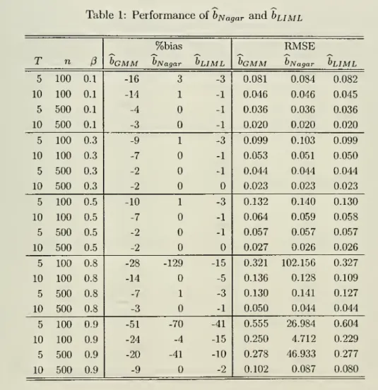
the conclusion follows.

In

Table

1,

we summarized

finite

sample

properties of h^agar

and

buML

approximated

by

10000

Monte

Carlo runs.^ Here,

_buML

is the estimator

where

As in (6) are replaced

by

the corresponding "eigenvalues". In general,

we

find that bj^agar

and buj^i

successfully

remove

bias unless /? is close to

one

and

the

sample

size is small.

4

Bias Correction

using

Higher

Order

Expansions

In the previous section,

we

explained the bias of the

GMM

estimator as a result ofthe biases

of the

2SLS

estimators. In this section,

we

consider elimination of the bias

by

adopting the

second order Taylor type approximation.

This

perspective has

been adopted

by Nagar

(1959),

and Rothenberg

(1983).

For this

purpose

we

first analyze the second order bias of

a

general

minimization

estimator 6 ofasingle

parameter

(3

&R

defined

by

b

=

argmin

Qn

(c) (7)

for

some

C

C

M.

The

score for the minimization

problem

is

denoted

by Sn

(c)

=

dQn

(c)/dc.

The

criterion function is

assumed

to

be

ofthe

form

_Q„

(c)

=

_g

(c)'

G

{c)~^

_g

(c)

where

_g(c)

and

G(c)

are defined in Condition 7.

The

criterion function

depends on

primitive functions 8 {wi,c)

and

V(tt;,,c)

mapping M^

x

M

into R"^ for

d

>

1,

where

Wi are i.i.d. observations.

We

assume

that

E

[6 {xL\,p)]

=

0.

We

impose

the following additional conditions

on

w^,6,

and

ip.

Condition

4 The random

variables

wi

are i.i.d.

Condition

5

The

functions 6{w,c)

and

tj;{w,c) are three times dijferentiable in c for c

£

C

where

C

CM

is a

compact

set such that (3

E

int

C.

Assume

that 6 {wi,c)

and

tp {iVi,c) satisfy a

Lipschitz condition \\6{wi, ci)

—

6{wi,C2)||

<

Ms

(wi)|ci

—

C2Ifor

some

function Ms{.) : IR'^

—

>

R

and

ci,C2

G

C

with the

same

statement holding for ip.

The

functions M5{.)

and M^(.)

satisfy

E

[Me

{wi)]

<

00

and

E

|M^

(wi)P

<

00.

Condition

6

Let Sj{wi,c)

=

d^6{wi,c)/dc^, '^ {wi,c)

=

ip {wi,c)il) {wi,c)'

and

'^j{wi,c)

=

d^^

{wi,c)

jdcK

Then, Xj (c)

=

E

_[6j {wi,c)],

and

Aj

(c)

=

E

_[^j (fOi, c)] all exist

and

arefinite

forj

=

0,...,3.

For

simplicity,

we

use the notation Xj

=

Xj _(/3),

Aj

=

Aj

(/?),

A

(c)

=

Xq(c)

and

A(c)

=

Ao(c).

Condition

7 Letg{c)

=

_-Yl'l^iS{wi,c),Qj {c)

=

^

Er=i

^j (""^^.c),

G

(c)

=

_^

_E"=i

_^

(^^i>c)

VK-,c)'

an

dGj{c)

= ^Er=i^iK,c).

Theng{c)

^

E[6iw„c)],

g,{c) -^

E[6,{w„c)],

G(c)

E

['^{wi,c)],

and

Gj

(c)

^

E

[i>-j{wi,c)] for all

ceC.

Our

asymptotic approximation

of the second order bias of b is

based

on an approximate

estimator b such that b

—

b

=

Op (^~^) -

The

approximate

bias ofb is then defined as

E

b

—

(3

while the original estimator h

need

not necessarily possess

moments

of

any

order. In order to

justify our

approximation

we

need

to establish that b is i/n-consistent

and

that

_Sn

(b)

=

with

probability tending to one. For this

purpose

we

introduce the following additional conditions.

Condition

8

(i) There exists

some

finite

<

M

<

00 such that the eigenvalues of

E

[^(zt;,-,c)] are contained in the

compact

interval

[M^-',M]

for all c

G

C;

(ii) the vector

E[8

{w^,c)\

=

if

and

only ifc

=

(3; (Hi) X\ 7^ 0.

Condition

9

There exists

some

r/

>

such that

E

Ms

{w^) ^

suPcecll^K'C)

|2+T7

<

00,

and

E

suPcGcllV'(^«i,c)f+''

<

00,

E

M^

(u'i)^2+7,

<

00,

<

00.

Condition 8 is

an

identification condition that guarantees the existence of a unique inte-rior

minimum

ofthe limiting criterion function. Condition 9 corresponds to

Assumption

B

of

Andrews

(1994)

and

is used to establish a stochastic equicontinuity property of the criterion function.

Lemma

1

Under

conditions 4 - _9, b defined in (7) satisfies y/n{b

—

(3)

=

Op(l)

and Sn

(6)

=

with probability tending to 1.

Proof.

See

Appendix

B.

Based on

Lemma

1 the first order condition for (7) can

be

characterized

by

A

second order Taylor expansion of (8)

around

/3 leads to

a

representation oi b

—

(3

up

to

terms

oforder Op{n~'^). In

Appendix

B, it is

shown

that

VS(6 -

ffl

=

-i*

+

-L (-ir

+

i*=

-

i;*')

+

Op

(-1=)

(9)

(See Definition 2 in

Appendix

B

for the definition of

*,T,$,H,

and

F.) Ignoring the Op

(A^j

term

in _(9),

and

taking expectations,

we

obtain the

"approximate

mean"

of ^/n{b

—

(3).

We

present the second order bias ofb in the next

Theorem.

Theorem

3

Under

Conditions 4-9, the second order bias

ofb

is equal to

(10)

where

E[T]

=

2tTace{A''E

and

E[^=]

=

SX[A-^E

E[^]

=

0, f\cf"1_\

6i^

_j

-

2X[A-^E

[^p^i>',A-H^]

-

trace

(A-^AjA-^i?

[6i6'^) ,

A-^Ai

-

4XjA'^E

[6^X\A-'^^P,^'^

A^^Ai

and

-SX'^A-^E

[6i6'^

A-^AiA-^Ai

+

AX'^A'^E

[<5,<5',]

A^^Aa,

E[<l>^]=iX[A-^E[6^6'^A-'X^,

Proof.

See

Appendix

B.

Remark

1

For

theparticular case

where

ip,

=

_6i, i.e.

when

b is a

CUE,

the bias

formula

(10)

exactly coincides with

Newsy

and

Smith's (2000).

We

now

applythese generalresults to the

GMM

estimator ofthe

dynamic

panel model.

The

GMM

estimator

_bcMM

can

be

understood

to

be

asolution to the minimization

problem

mm

c \

n

m,

(c)

for c

G

C

where

C

is

some

closed interval

on

the real line containing the true

parameter

value

and

m,

(c) V ^^.T-\ [vIt-i C X.:T-a

_J

T7 ^-^ 2=1 Zi\Zii Zx,T~\Z,_{7-_j}

We

now

characterize the finite

sample

bias of the

GMM

estimator

be

mm

of the

dynamic

Theorem

4

Under

Conditions 1-3 the second order bias of

bcMM

is equal to

B1+B2

+

B3

_f

1

+

-n

\n

(11)

where

zx s

Bi

=

Tr^

ELY

trace

_((rr)''

T-")

B2

=

_-2Tf

_zti

_EL7

rr' (rr)-'

r--

(rf

)-i

r

^3

=

Tr^

^^j-/ ^fr^i

rr' (rr)-'

-B3.1 (t,s)

_(rf

)-i

rr

.

andTi

=

Er=i'rr'(rfr^rr.

Proof.

See

Appendix

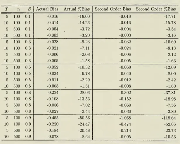
C.

In

Table

2,

we

compare

the actual

performance

oihcMM

and

theprediction ofits bias

based

on

Theorem

4.

Table

2 tabulates the actual biasofthe estimator

approximated

by

10000

Monte

Carlo runs,

and compares

it with the second order bias

based on

the

formula

(11). It is clear

that the second order theory does a reasonably

good

job except

when

p

isclose to theunitcircle

and

n

is small.

Theorem

4 suggests

a

natural

way

of eliminating the bias.

Suppose

that

Bi/B2,Bz

are

>/n-consistent estimators ofB-[,B2,B3.

Then

it is easy to seethat

t>BCi

—

t>GMM

{B-i

+

B2

+

Bsj

(12)

is first order equivalent to

_bcMM,

and

has

second

order bias equal to zero. _{Define Tf^}

=

n-'

HU

_^rt^tM""

=

ri-^

_EIli

_^rtKv

_^\T

=

«"'

_ELi

_{<t^l^u^is and}

n

i=l

where

e*j

=

y*^

—

x*^bGMM

Let

Bi,B2

and

.63

be

defined

by

replacing

rj^,rf^,r"^^ and

53,1(f,s)

by

ff

,fr,%"

and

53,i(i,s) in

Bi,B2 and

S3-Then

the

Bs

will satisfy the -yn-consistency requirement,

and

hence, theestimator (12) will

be

first order equivalent to

_bcMM

and

will

have

zero second order bias.

Because

the

summand

E

[z^tx*i]'

E

\z,t,z\^" 6*iZu\'^K^^Zisz[^E[z,sz[,]~

E

[zisX*,]

in the

numerator

ofi?3 is equal to zero for s

<

i,

we

may

instead consider

bBC2

=

bcMM

[

Bi

+

B2

+

B3

where

lis

=

tr^

eL"/

eI='

f

r' (f

f

) "' ^3,1(*,s)

(f

r

) ''

_f

r-Second

order asymptotic theory predicts

approximately

that 6j3C2

would be

relatively free

ofbias.

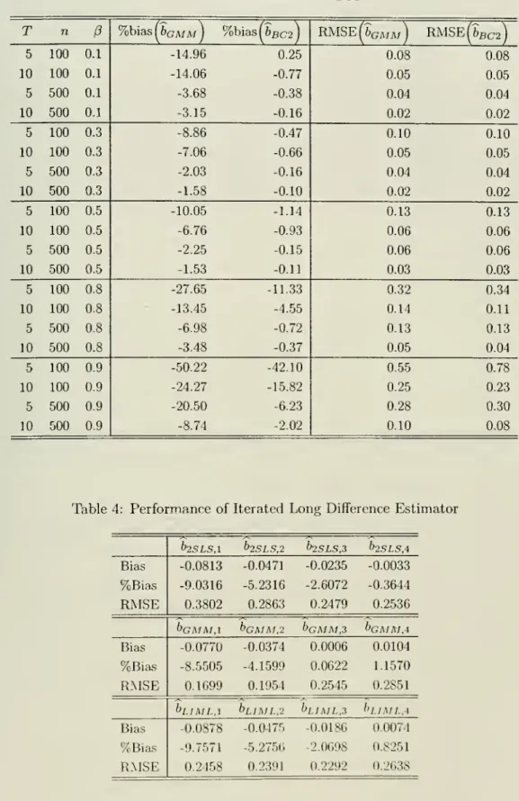
We

examined whether

such prediction is reasonably accurate in finite

sample

by

5000

Monte

Carlo runs.^ Table 3

summarizes

the properties of _6bc2-

We

have

seen in

Table

2 that the second order theory is reasonably accurate unless /3 is close to one. It is therefore sensible to conjecture that

bBC2 would have

a reasonable finite

sample

bias property as long as /3 is not

too close to one.

Such

a conjecture is verified in

Table

3.

5

Long

Difference

Specification:

Finite

Iteration

In previous sections,

we

noted that even the second order asymptotics "fails" to

be a

good

approximation

around

/?

~

1. This

phenomenon

can

be

explained

by

the 'Sveak instrument" problem. See Staiger

and

Stock (1997). Blundell

and

Bond

(1998) argued that the

weak

instru-ment

problem

can

be

alleviated

by assuming

stationarity

on

the initial observation yjo-

Such

stationarity condition

may

or"

may

not

be

appropriate for particular applications. Further,

sta-tionarity

assumption

turns out to

be

a

predominant

source ofinformation

around

/?

«

1 as

noted

by

Hahn

(1999).

We

therefore turn to

some

other

method

to

overcome

the

weak

instrument

problem around

theunit circle avoiding thestationarity assumption.

We

argue that

some

ofthe

difficulties of inference

around

the unit circle

would

be

alleviated

by

taking a long difference.

To

be

specific,

we

focus

on

asingleequation

based

on

the longdifference

VtT

-

yn

=

P

iViT-i

-

Vio)

+

{£iT

-

£n)

(14)

It is easy to see that the initial observation y,o

would

serve as a valid instrument.

Using

similar intuition asin

Hausman

and

Taylor (1983) or

Ahn

and Schmidt

(1995),

we

can

see that

2/iT-i

-

l3yiT-2, , yi2

—

Pyn

would be

valid instruments as well.

5.1

Intuition

In

Hahn-Hausman

(HH)

(1999)

we

found that the bias of

2SLS

(GMM)

depends on

4

fac-tors: "Explained" variance of the first stage

reduced form

equation, covariance

between

the

stochastic disturbance ofthe structural equation

and

the reduced

form

equation, the

number

of

instruments,

and sample

size:

„,:_,

_{_}

m

~

₁

(number

ofinstruments) x ("covarianc e")

n

"Explained" variance of the first stagereduced

form

equation

"The difTcrence of Monte Carlo runs here induced some minor numerical difference (in properties of

bcMM)

Similarly, the

Donald-Newey (DN)

(1999)

MSE

formula

depends

on

the

same

4factors.

We

now

consider first differences

(FD)

and

long differences

(LD)

to see

why

LD

does so

much

better in

our

Monte-

Carlo experiments.

Assume

that

T —

A.

The

first difference set

up

is:

2/4

-

Z/3

=

/?(ya

-

y2)

+

£4

-

£3 (15)

For the

RHS

variables it uses the instrument equation:

ys

-

y2

=

(/?

-

1)2/2

+

a

+

£3

Now

calculatethe

R^

forequation (15) using the

Ahn-Schmidt

(AS)

moments

under

"ideal

con-ditions"

where

you

know

(3inthe sense that the nonlinearrestrictions

become

linear restrictions:

We

would

then

use (y2, yi,yo,cv-f-ei,

a

-I-£2) asinstruments.

Assuming

stationarity forsymbols,

but

not using it as additional

moment

information,

we

can

write

yo

=

_Yzrp

+

^0'

where

^0

^

(0' -iln^ )• ^^ ^^^ t>e

shown

that the covariance

between

the structure error

and

the first stage error is

—

o"^,

and

the "explained variance" in the first stage is equal to

cr'^-^r^-Therefore,the ratio that determines the bias of

2SLS

is equal to

-a2

l

+

_p

2^±1

1-/3'

which

is equal to

—19

for /?

—

.9. For

n

=

100, this implies the percentage bias of

Number

ofInstruments

—19

,„„ 5

—19

_,„„ ,^^ ^^

:^ ;

—

7; TT-

X

100

=

——

-—

r x

100

=

-105.56

Sample

Size

_p

100 0.9

We

now

turn to the

LD

setup:

y4-yi

=

P

(ys

-

yo)

+

£4-£i

It

can be

shown

that the covariance

between

the first stage

and

second stage errors is

—

/3^(T^,

and

the "explained variance" in the first stage is given

by

—a

(2/3^

-

4/3''

-

2/3^

+

4/32

+ 4p-2p^

+

6)a^

+

P^

-p^ +

2-

2/3^

(-2/3-3

+

/?2)a2-l+/32

2

where

a^

= %.

Therefore, the ratio that determines the bias is equal to

2

{-2p-3 +

p^)a^-\+p^

(2/3^

-

4/3^

-

2/3'^

+

4/32

+

4/3

-

2/3^

+

6)a'^

+

/?^

-

p'^

₊

₂

_-

_2p^

which

is equal to

2.570

3x10-''

-.374

08

+

a2

+

4.8306x

IO-2

for /?

=

.9.

Note

that the

maximum

value that this ratio

can

take in absolute

terms

is

-.37408

which

is

much

smaller

than

—19.

We

thereforeconclude that the longdifferenceincreasesi?^

but

decreases the covariance. Further, the

number

of instruments is smaller in the long difference

specification so

we

should expect

even

smaller bias.

Thus,

all ofthe factorsin the

HH

equation,

except

sample

size, cause the

LD

estimator to

have

smaller bias.

5.2

Monte

Carlo

For the longdifferencespecification,

we

can

usey^o aswell asthe "residuals" yir-i

—

l3yiT-2-, -• -,

yi2—f3yii as validinstruments.^

We

may

estimate

p

by

applying

2SLS

tothelongdifference

equa-tion(14) usingyioasinstrument.

Wemaythenuse

(yio,yiT-i

-b2SLsyiT-2,

,yi2

-hsLsyn)^

instrument to the long difference equation (14) to estimate p. Call the estimator b2SLS,i-

By

iterating this procedure,

we

can define 62SL5,2, i>2SLS,Si Similarly,

we

may

first estimate /?

by

the Arellano

and Bover

approach,

and

use (yio,yiT-i

-bGMMyiT-2,

--

,yi2

-bcMMynj

as

instrument to the long difference equation (14) to estimate p. Call the estimator 6251,5,1•

By

iterating this procedure,

we

can

define

bGMM,2, ^GMM.s,

-- Likewise,

we

may

first estimate

P

by

_huML,

and

use [yio,yiT-i

-

buMLyiT-2,

,yi2-

buMLynj

as instrument to the long

difference equation (14) to estimate p. Call the estimator

bijML^-

By

iterating this procedure,

we

can

define bLiML,2, bLiML,3, --

We

found

that such iteration of the long difference

esti-mator

works

quite well.

We

implemented

these procedures for

T

=

5,

n

=

100,

p

=

0.9

and

(j^

=

o"^

=

1.

Our

finding with

5000

monte

carlo runs is

summarized

in Table 4. In general,

we

found

that the iteration ofthe long difference estimator

works

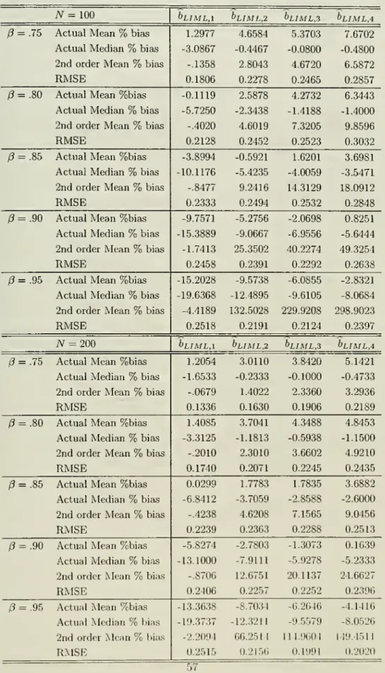
quite well.^

We

compared

the

performance

ofour estimator with Blundell

and Bond's

(1998) estimator,

which

uses additional information, i.e., stationarity.

We

compared

four versions oftheir

estima-tors bsBi, ,

bsBi

with the long difference estimators

bu

m

lATbu

m

L,2,bu

m

l,2,- For the exact

definition of 6bbi, , 6bb4, see

Appendix

E.

Of

the four versions,

6bb3 and bsBi

are the ones

reported in their

Monte

Carlo section. In our

Monte

Carlo exercise,

we

set

p

=

0.9, a^

=

\, Q.i r^

N

{0,1).

Our

finding

based

on 5000

Monte

Carlo runsis contained in

Table

5. In terms of

bias,

we

find that Blundell

and Bond's

estimators

_{6bb3 and 6^54 have}

similar properties as the

long difference estimator(s), although the former

dominates

the latter in

terms

of variability.

We

acknowledgethat theresidualinstruments are irrelevant underthe near unity asymptotics.

^Second order theory does not seem toexplain the behavior ofthe long difference estimator. In Table 7, we

comparethe actual performance ofthe long difference based estimators with the second order theory developed

(We

note, however, that

_{6bbi and 6bs2}

are seriously biased.

This

indicates that the choice ofweight

matrix

matters in

implementing

Blundell

and

Bond's

procedure.)

This

result is not

surprising

because

the long difference estimator does not use the information contained in the

initial condition. See

Hahn

(1999) for a related discussion.

We

also

wanted

to

examine

the

sensitivity ofBlundell

and

Bond's

estimator to misspecification, i.e., nonstationary distribution

of_yio- For this situation the estimator will

be

inconsistent. In order to assess the finite

sample

sensitivity,

we

considered the cases

where

yio

~

f

_j3k~

'

j^L

)

Our

Monte

Carlo results

based

on 5000

runs are contained in

Table

6,

which

contains results for (3p

—

.5

and

_^p

=

0.

We

find that the long difference estimator is quite robust,

_{whereas 6^53 and 6bb4}

become

quite

biased as predicted

by

the first order theory.

(We

note that

hBB\

and

_6bb2

are less sensitive

to misspecification.

Such

robustness consideration suggests that choice ofweight

matrix

is not

straightforward in

implementing

Blundell

and Bond's

procedure.)

We

conclude that the long

difference estimator

works

quite well

even

compared

to Blundell

and

Bond's

(1998) estimator.^

6

Near

Unit

Root

Approximation

Our

Monte

Carlo simulationresults

summarized

inTables1, 2,

and

3 indicate thatthe previously discussed

approximations

and

the biascorrections that are

based

on

them

do

not

work

well near the unit circle.

This

is

because

the identification of the

model becomes

"weak"

near the unit

circle. See Blundell

and

Bond

(1998),

who

related the

problem

to the analysis

by

Staiger

and

Stock (1997). In this Section,

we

formally

adopt approximations

local to the points in the

parameter

space that are not identified.

To

be

specific,

we

consider

model

(1) for

T

fixed

and

n

—

> 00

when

also /?„ tends to unity.

We

analyze the bias of the associated

weak

instrument limit distribution.

We

analyze the class of

GMM

estimators that exploit

Ahn

and

Schmidt's (1997)

moment

conditions

and

show

that a strict subset of the full set of

moment

restrictions

should

be

used in estimation in order to

minimize

bias.

We

argue that this subset of

moment

restrictions leads to the inference

based

on

the "long difference" specification. Following

Ahn

and Schmidt

we

exploit the

moment

conditions

E[uiu[]

=

{al

+

cTl)l

+

alll'

E

[uiyiQ] cr.

ayo-with

1

=

[1,.-.,1]' a vector of

dimension

T

and

Uj

=

[u,i,•j^^zt]

be

written

more

compactly

as

The

moment

conditions can

chE[uiu'^\ ₂ vech/ 9 vech(7

+

ll')

E

[uiyio]

=

<^e

+

^a

+

O'oyo

1

(16)

^We

did try tocompare thesensitivity ofthe two

moment

restrictionsby implementing

CUE.

but we experi-enced some numericalproblem. Numerical problem seemstobe an issuewith

CUE

in general. Windmeijer (2000) reports similar problemswith

CUE.

where

the

redundant

moment

conditions

have

been eHminated

by

use ofthe

vech

operator

which

extracts the

upper

diagonal elements

from a symmetric

matrix. Representation (16)

makes

it

clear that thevector b

E

R^(^+^)/2+^

is contained in

a

3 dimensional

subspace which

is another

way

ofstating that there are

G

=

T{T

+l)/2

+

T

—

3 restrictions

imposed

on

b.

This statement

is equivalentto

Ahn

and

Schmidt's (1997) analysis ofthe

number

of

moment

conditions.

GMM

estimators are obtained

from

the

moment

conditions

by

eliminating the

unknown

parameters

(T^,<y1,

and

Oay^.

The

setofall

GMM

estimators leadingto consistent estimatesof/?

can

therefore

be

described

by

a

{T{T

+

l)/2

+

T)

x

G

matrix

A

which

contains all the vectors

spanning

the orthogonal

complement

of6.

This

matrix

A

satisfies b'A

=

0.

For our purposes it will

be

convenient to choose

A

such that

b'A

=

[EuitAuis,E

{uiT^Uij),

EuiAuik,

EAu'^yio] ,

s

=

2,...,T;i

=

l,...s-2;j

=

2,...,r-l;A;

=

2,...,T

where

Aui

=

[ui2

—

un,

...,Uix

—

UiT-i] It

becomes

transparent that

any

other representationof

the

moment

conditions

can

be

obtained

by

applying acorresponding nonsingularlinear operator

C

tothe

matrix

A.It

can

be

checkedthat thereexistsa nonsingular

matrix

C

such that b'

AC

=

is identical to the

moment

conditions (4a)-(4c) in

Ahn

and Schmidt

(1997).

We

investigate the properties of (infeasible)

GMM

estimators based

on

E

[u^tAuis (/?)]

=

0,

S

[u^T^Uij (/?)]

=

0, £;[u,Au,k (/?)]

=

0,

S

[Vro^u.t (/?)]

=

obtained

by

setting

Auu

{(3)

=

Ayu -

PAyu-i-

Here,

we

assume

that the instruments

uu

are

observable. Let

gn

{(3) denote a

column

vector consisting

oiuuAuis

(/3) ,

UixAuij

(/?)

,UiAuik

(/?).

Also let g,2{(3)

=

[y^oAu,{f3)]. Finally, let

_gn{P)

=

n-^^j:^^,

_{[g^l (P)'}

,9^2 {P)']'

with

the

optimal weight

matrix

fin

=

E

[gi (/?„) gi (/?„)'].

The

infeasible

GMM

estimator of a possibly

transformed set of

moment

conditions

C'gn

(/?) then solves

P2SLS

=

argmin

g„(/3)'

C

(C'C!„C)+ C'gn

_{{(3) (17)}

where

C

is a

G

x r

matrix

for 1

<

r

<

G

such that

C'C

=

_U

and rank (c{C'Q,C)'^ C'\

>

1.

We

use [C'Q.C)'^ to denote the

Moore- Penrose

inverse.

We

thus allow the use of a singular

weight matrix.

Choosing

r less

than

G

allows to exclude certain

moment

conditions. Let

ki

=

-dgii{0)/dp,

/,,2

=

-%2(/?)/a/?,

and

/„

=

_n-^^Z^^i

_[fuJ^]'-

The

infeasible

2SLS

estimator can

be

written as

P2SLS

-Pn=

(fnC

(G'fi„G)+

C

fX'

_f^C

_{(C'fi„G)+ C'gn}

iPn) (18)

We

are

now

analyzing the behavior _{of /?2sl5}

-

_Pn

under

local to unity asymptotics.

We

make

the following additional assumptions.^

Condition 10

Let

yu

=

Oi

+

PnVit-i

+

^it with

en

~

A'' (0,cr^), ai

^

N

(0,a^)

and

y^o

~

A'' (

^%

,

j^^

],

where

/?„

=

exp(—

c/n) for

some

c

>

0.

Also note that

Ayu

=

Pl^^Vio

+

^it

+

^

_El=i

Pn'^^u-s

+

Op(n-^)

where

r?,o~iv(0,(^„-l)y

(1-/32)).

Under

the generating

mechanism

described in the previous definition the following

Lemma

can

be

established. '

Lemma

2

Assume

/?„

=

exp(—

c/n) for

some

c

>

0.

For

T

fixed

and

as

n

-^ oo

i=l i=l

and

where[!i'^,i'y]

~

iV(0,E) with

E

Ell Ei2 E21 E22

and

Ell

=

^I, E12

=

SMi

E22

=

SM2,

where

2 2

Ml

=

-1 1

and

S12

=

E21.

We

also have

1

-1

M2

2

-1

•-

_-1

-1 2 1

_^

\ ^ E22

+

o(l)

Proof.

See

Appendix

D.

Using

Lemma

(2) the limiting distribution of

P2SLS

~

Pn

is stated in the next corollary. For this

purpose

we

define the

augmented

vectors

_^f

=

[O,...,0,^^]

and

^*

=

[O,...,0,^^]

and

partition

C

=

[C'qjC{]' such that

C'^f

=

C[^^. Let rj denote the

rank

_{of Ci.}

Corollary

1 Let

_P2SLS

" Pn

^^ given by (IS). IfCondition 10 is satisfied then

d

SiCl (C1S22C1)

C{^y

P:2SLS

-

1

c;ci(C5E22Circ;e

=

^V(C,S22)

(19)

Unlike the limiting distribution for the

standard

weak

instrument problem,

X(C,

E22), as

defined in (19), is

based

on

normal

vectors that

have

zero

mean. This degeneracy

is generated

by

the presence of the fixed effect in the initial condition, scaled

up

appropriately to satisfy

the stationarity requirement^'' for the process yu- Inspection ofthe proof

shows

that the usual

concentration

parameter

appearing in the limit distribution is

dominated by a

stochastic

com-ponent

related tothe fixedeffect.

This

situation

seems

to

be

similar to

time

series

models

where

deterministic trends can

dominate

the

asymptotic

distribution.

Based

on

Corollary 1,

we

define thefollowing classof

2SLS

estimatorsfor the

dynamic

panel

model.

The

class contains estimators that only use

a

nonredundant

set of

moment

conditions

involving the initial conditions _yiQ.

Definition

1 Let

_P2SLS

^^ _{defined as P^gj^g}

=

argmin^

^2,n(/?)'

_Ci

lC{QCi)

C[g2,n{0),

where

92,71(0)

=

Ti~^'^_Yl^=\ 9i2{P)r

^

is a

symmetric

positive definite

(T

—

1)

x

(T

—

1)

matrix

of

con-stants

and C\

is a

[T

—

\)

X

r\

matrix

offull

column rank

rj

<

T

—

1 such that

_C[Ci

=

I.

Next we

turn tothe analysis ofthe asymptotic bias for the estimator

_P2SLS

^^the

dynamic

panel model. Since the limit only

depends on

zero

mean

normal

random

vectors

we

can apply

the results of

Smith

(1993).

Theorem

5 Let

X*

_(Ci,QJ

be the limiting distribution of

_P2SLS

~

1 i''^ Definition 1

under

Condition 10. Let

D

=

[D

+

D')/2, where

D

=

(c{QCi]

C[M[Ci.

Then

[x

(c„n)] =

A-

_f;

<MWc»

(fl,/n

-

A- {c[acX')

fc=0 \2)\+k'^- V

^ _^

/

E

'"An alternative way to parametrize the stationarity condition is to set yu

=

(!—/?„)Qi

+

(B^yu-i

+

en,

£it

~

N

(O.CTj) ,Qi

~

N

{0,al) andy.o

~

N

iOi,

_y^^

_j with/3„

=

exp(-c/n).It canbeshownthatanestimator

soley based on the

moment

condition E[uii^Uik(Po)]

=

is consistent. Restrictingattention toestimators that are ba.sed on all

moment

conditions except the conditionE[uiAu,k_(/3o)]

=

0, onecan show that

wherefi

=

It-icry/2.Estimatorsintheclass /Jjs^s definedinDefinition1 canbeanalyzed bythesame methodsas

underthestationarityassumptionsdiscussedin thepaper. Theirlimiting distributions aredenotedby

X'

(Ci, )

.

Moments

oi

X*

areintractably complicated unlessQ,

=

It-\- Then the mean of

^*

(Ci,/t-i) is givenby

^i'D^J

„,r-l

r-l

^l'n n'D^i_,_

^,r-l

r-1

r+1

'^'(^-•^

+

i'^)-7TT^"^^^^~^'^-

+

'>~-with

D

=

[D

+

D

)/2,

D

=

C[MiC-i and /i

=

C\ij.. Whilefindingan exact analytical

minimum

ofthe abovebias

expression as a function ofthe weight matrix is probably infeasible due to the complexity of the formula, one sees relatively easily that for large

T

the

minimum

must approximately be achieved for

C

=

lr~i, thus leading approximatelytothe long difference estimator.

where

_n

=

rank(Ci),

(a)j, is the

Pochammer

symbol

r{a

+

b)/r{b),

C^^{.,.)

is a top order invariant

polynomial

defined by

Davis

(1980)

and A

is the largest _{eigenvalue of}

(c[ClC]\

.

The

mean

E

X

[Ci,^)

exists_forr\

>\.

Proof.

See

Appendix

D.

The Theorem

shows

that the _{bias of /?2sl5}

both depends on

the choice of

C\

and

the weight

matrix

^.

Note

fore

example

that

E[X{C\,It-\)]

=

txD/r\.

The

problem

of

minimizing

the bias

by

choosing optimal matrices

C\

and

Vt

does

not

seem

to lead to

an

analytical solution

but

could in principle

be

carried out numerically for a given

number

of

time

periodsT. For our

purpose

we

arenotinterested insuch

an

exact

minimum.

We

show

however

that for

two

particular choices ofQ.

where

Q,

=

It-\ ox Q.

=

II22

and

subsequent

minimization

over

C\ an

analytical solution for the bias

minimal

estimator can

be

found. It

turns out that the

optimum

is the

same

for

both

weight matrices.

The

theorem

also

shows

that the

optimum

can

be

reasonably well

approximated

by

a procedure that is very easy to

implement.

Theorem

6

Let

X

(Ci,Qj

be as defined in Definition 1. Let

D

=

{D

+

D') /2

where

D

=

{C[

ncX^

C[

M[

Ci

.

Then

c

st'i'^c I

\E{^(CuIt^,)]\=

min

\E

[X

{Cu^22)]\

-Oi 5.1. OjL-i

=

J7-j Ci s.i. GjGi=irj

ri=l,..,r-l Ti

=

l,..,T-l

Moreover,

E[X{CiJT-i)]

=

tTD/r^.

Let

_CI

=

argmin^^j \E

[X{CiJt-\)]\

subject to

C[Ci

=

Ir^,ri

=

1,

..,T-

1.

Then C^

=

_Pi

where

/9j is the eigenvector corresponding to the smallest eigenvalue li of

D.

Thus,

mincitx D/ri

=

min/,/2.

As

T

-^ 00 the smallest eigenvalue of

D,

minli

—

> 0. Let 1

=

[1,...,1]' be a

T—1

vector.

Then

for

Ci

=

l/(l'l)^/^ itfollows that tr

D

-^ as

T

-^ 00.

Theorem

6

shows

thattheestimator that

minimizes

thebiasis

based

only

on a

single

moment

condition

which

is a linear

combination

ofthe

moment

conditions involving j/jQ as instrument

where

the weightsare the elementsoftheeigenvector_p^ correspondingtothesmallesteigenvalue

of

(Ml

+

Mj)

/2.

This

eigenvalue can

be

easily

computed

for

any

given T.

The

Theorem

also

shows

that at least for large

T

a

heuristic

method

which

puts equal weight

on

all

moment

conditions leads to essentially the

same

bias reduction as the optimal procedure.

The

heuristic

procedure

turnsout

be

equal tothe

moment

condition

E

{{uiT

—

"n)

yio]

which can be motivated

by

taking"long difTerences" ofthe

model

equation yu

=

cti

+

_{/?„yit_]}

+

en

i.e.

by

considering

It can also

be

shown

that a

2SLS

estimatorthat uses all

moment

conditions involving?/,o

remains

biased even as

T

—

> 00.

7

Long

Difference

Specification:

Infinite

Iteration

We

found

that the iteration ofthe long difference estimator

works

quite well. In the {i

+

l)-th

iteration, our iterated estimator estimates the

model

ViT

-

yn

=

PiViT-i

-

Uio)

+

£iT

-

ea

based on

2SLS

using instruments Zi _{^(^e))

—

{yi0,yi2

-

P{e)yn,--- ,yiT-i

-%)?/ir-2J, where

P,(\ is the estimator obtained in the previous iteration.

We

might want

to

examine

properties of

an

estimator

based on an

infinite iteration,

and

see if it improves the bias property. If

we

continue the iteration

and

it converges^

\

the estimator is a fixed point to the minimization

problem

where

^i{b)

=

Zi(b) _{{yiT

—

_yii)

—

b{yir-i —yio))- Call the

minimizer

the infinitely iterated

2SLS

and

denoteit _I3j2Sls-

Another

estimator

which

resembles

_Pj2sls

i^

CUE,

which

solves

(N

\'

_/ '^

\~^

/

^

{b)

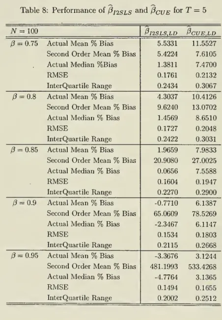
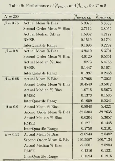
Their actual

performance

approximated

by 5000

Monte

Carlo runs along with the biases

pre-dicted

by

second order theory in

Theorem

4 are

summarized

in Tables 8

and

9.

We

find that

the long difference

based

estimators

have

quite reasonable finite

sample

properties even

when

/?

is close to 1. Similar tothefiniteiteration in the previoussection, thesecond order theory

seem

to

be

next to irrelevant for /3close to 1.

We

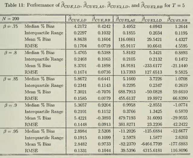
compared

performances

ofour estimators

with

Ahn

and

Schmidt's (1995) estimator as

well as Blundell

and Bond's

(1998) estimator.

Both

estimators are defined in two-step

GMM

procedures. In order to

make

a accurate

comparison with

our longdifference strategy, for

which

thereis

no

ambiguity

ofweight matrix,

we

decided toapply the continuous

updating

estimatorto

their

moment

restrictions.

We

had

difficulty of finding global

minimum

for

Ahn

and

Schmidt's

(1995)

moment

restrictions.

We

therefore used a

Rothenberg

type

two

step iteration,

which

would have

the

same

second order propertyasthe

CUE

itself. (See

Appendix

I.) Again, in order

to

make

a accurate comparison,

we

applied the

two

step iteration idea toour long difi"erence

and

Blundell

and

Bond

(1998) aswell.

We

call theseestimators

_Pcue2

_aSj

_PcuE2

_ld^

^^^

_0cuE2

BB-We

set

n

=

100

and

T

=

5.

Again

the

number

of

monte

carlo runs

was

set equal to 5000.

Our

results are reported in Tables 10

and

11.

We

can

see that the long difference estimator has a

comparable

property to

Ahn

and

Schmidt's estimator.

We

do

not

know

why

_Pcue2LD

^^^ such

alarge

median

bias at /3

=

.95

whereas

P^y^

_iq

does not have such problem.

"Thereisnoapriori reasonto believe that the iterationsconverge tothefixed point. To show that,onewould

8

Conclusion

We

have

investigatedthebias ofthe

dynamic

panel effects estimators using

second

order

approx-imations

and

Monte

Carlo simulations.

The

second

order

approximations

confirm the presence

ofsignificant bias as the

parameter

becomes

large, ashas previously

been found

in

Monte

Carlo

investigations.

Use

ofthesecond order asymptotics todefine asecond order unbiased estimator

using the

Nagar

approach

improve

matters,

but

unfortunately does notsolvetheproblem.

Thus,

we

propose

and

investigate a

new

estimator, thelongdifferenceestimatorofGriUches

and

Haus-man

(1986).

We

find in

Monte

Carlo

experiments

that thisestimator

works

quitewell,

removing

most

ofthe bias

even

for quite high values ofthe parameter. Indeed, the long differences

esti-mator

does considerably better

than

"standard" second order asymptotics

would

predict.

Thus,

we

consider alternative asymptotics

with a

near unit circle approximation.

These

asymptotics

indicate that the previously

proposed

estimators for the

dynamic

fixed effects

problem

suffer

from

larger biases.

The

calculations also

demonstrate

that the longdifference estimator should

work

in eliminating the finite

sample

bias previously foimd.

Thus,

the alternative asymptotics explain our

Monte

Carlo finding ofthe excellent

performance

ofthe long differences estimator.

Technical

Appendix

A

Technical

Details

for

Section

3

Lemma

3

E

_{E{<^'-:-^/.'«":)}

Proof.

We

have

E

xl'Ptel

- ^xl'Mte:

E{tTa.ce{PtEt[e:x;'])]

Kt

0.

-E

[trace{MtEtlelx*/])],

n-Kt

whereEt[] denotesthe conditionalexpectation givenZt- Because Et[el]

=

0, Et[e^xl']istheconditional

covariancebetweene^ and_yl'-i,whichdoes not depend onZtdueto jointnormality. Moreover, by

cross-sectional independence,

we

have

Et [e;xr]

=

Et [eltxlt] /„.

Hence, using the fact that trace (Pj)

=

Kt

and trace(Mj)

=

n

—

Kt,

we

have

xl'Pte;

-

—x'Mtc

n

Et

[eltxU

{Kt

-^^^

[n

-

Kt)^

=

0,

from which theconclusion follows.

Lemma

4

Var{xl'Mte;)

=

{n

-

t)

a^E

[v*^]

+

[n

-

t)

{E

_[<,e*J)'

,

Cov

[xl'h'Itel,x'/Msel)

=

{n

-

s)

E

[vie*,]

E

[<,£*,]

,

s<t

wherev*,

=

x*,

-

E[x\,\zn].

Proof. Follows by modifying the developments from (A23) to (A30) and from (A31) to A(34) in

Alvarez and Arellano (1998).

Lemma

5 Suppose that s

<

t.

We

have

E

\v^]

=

T

-t

/ 1

0-0

T-t+l ^2

T-t

1 "

_T-t

₊

l(T-tf{l-pf

X

\{T-t)

+

r-1

E[vy*,]

=

-o^

+

fT^ /

T

-0"-)

\JT-

i

+

1 (T

-i t){\ 1

~0)

T~t

T-i

+

l{T-tf{l-0)

[T-t]

0-0

1

-E[vle*^]

=

-a

+

a'

.^/

'

-s

i}

-P^-

J '

_Vr-

-_s

+

₁ (T --_s -5)(1 1

-P)

\It-s

+ \{T-i

)(r-1 t){\-

_-P)

1

T--t

E

Kel]

^

Y

T

-

f

+

1

(T

-

5)(r

-

t) (1

-

/?)

(T-t)

T-t

\-p

T-t

1-/?

;'

1-/3

Proof.

We

first characterize v*j.

We

have

Xi,t

=

J/i.t-i

Xi,t+i

=

Vi.t

=

Qi

+

Pyi,t-\

+

£i,t

i,r

=

yi,r-i

=

—

i

^-Qi

+

P'^ *yi,t-i

+

ffi,T-i

+

Pei,T-2

+

+

P"^ ' _^e^.t)

1

—

_p

\ / and hence

T-f

+

l , 1 ,

P-P

T-f+l yi,t-i /?-/?T-t+l ^

(T-i)(l-/3)y^"'-^

\l-/3

(r-i)(l-/3)V

(1

-

P)£i,T-i

+

(1

-

/3^)ei,T-2

+

+

(l

-

Z?"^-*)ei,t

(T-i)(l-/?)

It followsthat

1 /?-/?T-t+l

T-t

from which

we

obtain

T-t

{T-t){l-p)

J

''•'-'

yi-P

(T-t)

(1-/3)2^ E[ai\zit], 1 (ai -£'[Qi|2,i])

T-t

+

l

yi-p

{T-t){l-pf

J

T-t

(1

-

/3)^..T-i

+

(1

-

/?')£i,r-2

+

•••+(!-

P'^-')

{T-t){\-P)

T-t

+

l (20)

We

now

compute

E

(Qj

-

E\ai\zit\y Var[q;!Zit]. It canbe

shown

that

2 2

Cov(Q„(y,o,-..,y.(-i)')

=

_Y^^>

and Var ((y,o, - ,2/zt-i)')

=

—

^^^^'

+

Q

where £ is a i-dimensioanl column vector of ones, and

Q

I-

p' t-2 1

P

P'

P

1

P

21