Comparative Analysis of Automotive Powertrain
Choices for the Near to Mid-Term Future
by
Emmanuel P. Kasseris
Diploma in Mechanical Engineering
Aristotle University of Thessaloniki, Greece 2004
SUBMITTED TO THE DEPARTMENT OF MECHANICAL ENGINEERING IN PARTIAL FULFILLMENT OF THE REQUIREMENTS FOR THE DEGREE
OF
MASTER OF SCIENCE IN MECHANICAL ENGINEERING AT THE
MASSACHUSETTS INSTITUTE OF TECHNOLOGY JUNE 2006
@2006 Massachusetts Institute of Technology All rights reserved
Signature of Author: ...
Certified by: ...
Department ofhiechanical Engineering May 26, 2006
... ... ... ... ---John B.Heywood Sun Jae Professor of Mechanical Engineering visor Accepted by: ... MASSACHUSETTS INSITUTE.' OF TECHNOLOGY
JUL 14
2006
Lallit Anand Professor of Mechanical Engineering Chairman, Department Graduate Committee(This page was intentionally left blank)
Comparative Analysis of Automotive Powertrain
Choices for the Near to Mid-Term Future
by
Emmanuel P. Kasseris
Submitted to the Department of Mechanical Engineering on May 26, 2006 in Partial Fulfillment of the Requirements for the Degree of Master of Science in Mechanical
Engineering
ABSTRACT
This thesis attempts a technological assessment of automotive powertrain technologies for the near to mid term future. The powertrain types to be assessed include naturally aspirated gasoline engines, turbocharged gasoline engines, diesel engines, electric hybrids using gasoline engines and advanced transmissions. Advancements in aerodynamics, weight reduction and tire rolling friction are also taken into account.
The basis for the comparison is the potential of these powertrain technologies for reduction of oil consumption and green house gas emissions at the same level of performance as current vehicles.
The fuel consumption and performance of future vehicles was estimated using simple scaling laws and vehicle simulations. The results indicate that the potential for reduction of fuel consumption is significant for all the powertrains examined. More specifically, it seems that the current relative advantage of diesel over gasoline engines in terms of fuel consumption is reduced. Future turbocharged gasoline engines especially, seem to become almost equivalent with diesel engines. Hybrids electric vehicles do maintain a competitive advantage over other powertrains in terms of reduction of fuel consumption. This advantage is however much more pronounced for urban than for highway driving.
Thesis Supervisor: John B. Heywood
Acknowledgements
First of all, I would like to thank Professor Heywood for giving me the opportunity to work on this research project under his supervision. Except for a world-known expert on the field of engine and automotive technology, Professor Heywood is an amazing educator. He supported and guided me every step of the way. Working with him, I feel that I have gained valuable lessons not just in science and engineering but also in how engineering interacts with societal, economic and political forces in order to make an impact.
My eternal gratitude goes to my parents Vasiliki and Panayiotis, my sister Alexandra and the rest of my family for their support throughout my life. Nothing would have been achieved without their love.
The help of my co-workers on this research project Matthew Kroemer, Anup Bandivadekar, Lynette Cheah and Tiffany Groode has been priceless. Our interaction and cooperation on the problems encountered in our research has been ideal.
Finally I would like to thank my friends for their support and for making MIT a pleasurable experience.
Table of Contents
AB STRA CT... 3
Acknow ledgem ents... 5
Table of Contents... 6 List of Figures... 8 List of Tables ... 12 N om enclature... 13 Abbreviations... 14 1. Introduction... 16 1.1. M otivation... 16 1.2. Focus ... 19
1.2.1. W hat is a Pow ertrain ... ... ... . . 19
1.2.2. W hich Technologies Should be M odeled? ... ... . . 20
1.3. M ethodology ... 22
1.4. Testing Fuel Consum ption... 23
1.5. Literature Review ... 27
1.6. Ways to Reduce Automotive Fuel Consumption... 27
1.7. Thesis Outline ... 29
2. N on-Pow ertrain Im provem ents... 30
2.1. Introduction... 30
2.2. V ehicle Resistances ... 30
2.3. Im provem ents in V ehicle Aerodynam ics... 35
2.4. Im provem ents in Tire Rolling Friction... 40
2.5. Vehicle W eight Reduction... 41
3. Internal Com bustion Engines... 45
3.3. Introduction... 45
3.2. Advanced Naturally Aspirated Gasoline Engines... 46
3.2.1. Engine Efficiency M ap Evolution ... 46
M ethodology... 46
D ecom posing Current Engine M aps... 48
Future Engine Efficiency Im provem ents... 55
3.2.2. Power Density Improvements- Engine Sizing ... 58
3.3. A dvanced Turbocharged G asoline Engines... 62
3.3.1. M ap Evolution m ethodology ... 63
3.3.2. Sizing-Scaling m ethodology... 68
3.3.3. The Effect of Turbo Lag ... 71
3.4. A dvanced Diesel Engines ... 72
3.4.1. M ap Evolution m ethodology ... 73
3.4.2. Sizing-Scaling m ethodology... 78
4. Controls-Transm issions for ICE Pow ertrains ... 81
4.1. Introduction... 81
4.2. Background-How does a Manual or Automatic Gearbox Work?... ... . . 81
4.2.1. N orm al D riving O peration... 86
4.2.2. Perform ance Tests... 88
A cceleration Perform ance... 89
G rade and Towing Capability... 91
4.3. Background-How does a CVT Gearbox Work... 91
4.3.1. N orm al D riving Operation... 92
4.3.2. Perform ance Tests... 93
4.4. Choosing G earboxes for 2030 V ehicles ... 95
4.4.1. Type ... 95
4.4.2. G ear Ratios... 95
4.4.3. Transm ission Efficiencies... 99
4.4.4. G ear Shifting M ethodology ... 102
5. H ybrid Electric V ehicles... 104
5.1. Introduction... 104
5.2. Background ... 104
5.2.1. Ways in which an HEV Saves Energy-What is the Potential?... . . . 104
5.2.2. H ybrid A rchitectures... 105
Series A rchitecture... 106
Parallel A rchitecture ... 107
A Hybrid Architecture Combining Series and Parallel-The Power Split Architecture ... 109
5.3. A D V ISO R V alidation... 114
5.4. Choosing an A rchitecture ... 115
5.5. Com ponents-H ow will they evolve?... . . . 119
5.5.1. Engine ... 119
5.5.2. M otor... 119
5.5.3. Electrochem ical Energy Storage... 120
Current Status of H ybrid Battery Technology ... 121
Future Status of H ybrid Energy Storage Technology... 123
5.5.4. Regenerative Braking... 126
5.6. Controls... 128
5.7. Sizing M ethodology... 129
5.8. The effect of H R ... 133
5.9. G ear R atios Selection... 136
6. Results... 138
6.1. Current m odels -V alidation... 138
6.2. Tank to Wheels Combined adjusted HW-FTP Fuel Consumption... 140
6.3. Perform ance Results (0-60, 40-60)... 141
6.4. The Effect of Perform ance and Vehicle Type ... 143
6.5. The Effect of the D riving Cycle... 150
6.6. Sensitivity to Engine M ap A ssum ptions... 157
6.7. Sensitivity to CV T Efficiency and to Shift W indow ... 157
6.8. Sensitivity of H ybrids ... 159
6.9. Com parison w ith the Previous Study... 164
6.10. W ell to Tank results ... 167
6.11. O ther Perform ance Results ... 169
6.12. Conclusions-Future W ork... 172
Bibliography ... 175
List of Figures
Figure 1: U.S.A. Light Duty Sales Averaged Fuel Economy versus Model Year .Source:
[3 ]... 17
Figure 2: U.S.A. Light Duty Fleet Weight and Performance versus model year. Source: [3 ]... 18
Figure 3: U.S.A. Light Duty Fleet sales Fractions by Vehicle Type versus Model year. S o urce : [3]... 18
Figure 4: Fuel Consumption versus weight in lbs for two model years- 1974 and 2004. S ource: [3]... 19
Figure 5: A Vehicle Powertrain. Adapted from [4]... 20
Figure 6: Estimated Times for New Powertrain Technologies to Affect US transportation Energy U se, A dapted from [5]... 21
Figure 7: Schematic of Component Subsystems used in the ADVISOR simulations... 24
Figure 8: The FTP D rive Cycle ... 25
Figure 9: The HWFET Drive Cycle... 25
Figure 10: The U SO6 Drive Cycle ... 26
Figure 11: Example urban driving energy flows for a late-model midsize passenger car.28 Figure 12: Example highway driving energy flows for a midsize passenger car. Source: [16] ... 2 9 Figure 13: Vehicle moving at a velocity V up a hill. Adapted from [4]... 30
Figure 14: Aerodynamic and Rolling Resistances versus Vehicle speed... 32
Figure 15 : Aerodynamic and Rolling Resistances versus Vehicle speed for the 2005 4.2 liter Ford F 150 ... 33
Figure 16: Vehicle Resistances Including Grade for the 2005 2.5 liter Toyota Camry.... 33
Figure 17: Vehicle Resistances over the FTP driving Cycle for the 2005 2.5 liter Camry ... 34
Figure 18: Vehicle Resistances over the HWFET driving Cycle for the 2005 2.5 liter C am ry ... 34
Figure 19: Streamlines around a Moving Vehicle ... 35
Figure 20: Cross-Sectional area, definition, approximation and correlation with vehicle size ... 37
Figure 21: CD Evolution for Chrysler Models. Source:[17]... 38
Figure 22 Coefficient of Drag Evolution for GM Sedans. Source: [17]... 39
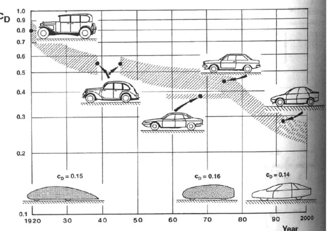
Figure 23: History of CD evolution for European passenger Cars compared with experimental prototypes. Source: [17]... 39
Figure 24: The deflection and rolling resistance... 40
Figure 25: Weight Reduction Opportunity for Different Materials at the vehicle level... 42
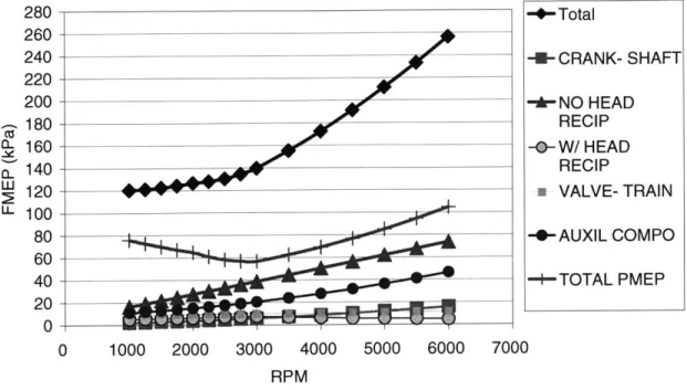
Figure 26: Fmep losses as a function of rpm. 5.4 liter Ford V8 Triton Engine used in the 200 5 F 150 . ... 50
Figure 27: 3.0 liter Toyota Camry Engine, BSFC Source: [29]... 51
Figure 28: Normalized Engine Brake Efficiency Map predicted by the friction m odel.2005 3.0 liter Camry Engine... 52
Figure 29: Normalized Engine Brake Efficiency Map predicted by the friction model... 52
Figure 30: Brake Specific Fuel Consumption Map predicted by the friction model... 53
Figure 31: Brake Specific Fuel Consumption Map predicted by the friction model... 53
Figure 33: Relative Error in BSFC between predicted and measured maps... 54
Figure 34: Relative Error in BSFC between predicted and measured maps... 55
Figure 35: Future Toyota Camry Brake Fuel Efficiency Map... 57
Figure 36: Future Ford F150 Brake Fuel Efficiency Map... 57
Figure 37: Historical evolution of engine powertrain density ... 58
Figure 38: Bmep Evolution for the case of the 2005 2.5 liter Camry... 61
Figure 39: Torque Evolution for the case of the 2005 2.5 liter Camry... 62
Figure 40 Manifold Intake Pressure for the Turbocharged Engine of the 2030 Camry 2.5 liter equivalent vehicle... 65
Figure 41 Exhaust Pressure for the Turbocharged Engine of the 2030 Camry 2.5 liter equivalent vehicle ... 66
Figure 42 Exhaust Temperature for the Turbocharged Engine of the 2030 Camry 2.5 liter equivalent vehicle ... 67
Figure 43 Brake Fuel Efficiency (qb,) and maximum bmep (corresponding to maximum torque) for the Turbocharged Engine of the 2030 Camry 2.5 liter equivalent vehicle ... 6 8 Figure 44: Maximum Torque curve comparison for NA-PFI, Turbocharged PFI and Turbocharged G D I... 70
Figure 45: Maximum T Curve for the 2030 Turbo SI lower performance Toyota Camry ... 7 1 Figure 46: Response to a step change In requested torque for a NA SI-PFI, a turbo PFI and a turbo GDI engine. Adapted from SAE [41]... 72
Figure 47: W illan's Line Technique... 74
Figure 48: Validation of the assumption of constant tq and fmep=F(N) only. ... 74
Figure 49: Dependence of fmep on bmep and speed for the 2005 Cummins Diesel Engine, assum ing constant % ... 75
Figure 50: Current Diesel Engine Map and maximum engine bmep. ... 76
Figure 51: Comparisons between European and U.S. emissions standards ... 77
Figure 52: Diesel Engine map for the 2030 diesel lower performance Camry indexed by b m ep ... 7 8 Figure 53: Historical Evolution of Diesel Volumetric Power Density... 79
Figure 54: Diesel Engine map for the 2030 diesel lower performance Camry indexed by torq u e ... 80
Figure 55: Ideal Powerplant Torque and Power versus speed Curves. Adapted from [4]83 Figure 56: Tractive Effort for an ICE Powerplant and a 4spd manual Transmission. A dapted from [4]... 83
Figure 57: Schematic of Hydraulic Torque Converter. Adapted from [4] ... 84
Figure 58: Characteristics of a Hydraulic Torque Converter. Adapted from [4]... 85
Figure 59: Tractive Effort for an ICE powerplant and a 3spd Automatic Transmission. A dapted from [4]... 86
Figure 60: The effect of Gear Shifting on Engine Operating Points ... 87
Figure 61: Operating Points for the 2005 2.5 liter Camry during the FTP... 87
Figure 62: Engine Operating Points during 0-60mph Acceleration. ... 89
Figure 63: Maximum Vehicle Speed Calculation for the 2005 2.5 liter Camry... 90
Figure 65: Comparison of Engine Operating Points when using a CVT and an Automatic
Gearbox. Adapted from [45]... 92
Figure 66: Engine Operating Points During 0-60 mph Acceleration For the 2005 2.5 liter C am ry U sing a C V T . ... 93
Figure 67: Total gear ratio during a 0-60 mph acceleration for a CVT ... 94
Figure 68: Total gear ratio during a 0-60 mph acceleration using an Automatic T ransm ission ... 94
Figure 69: Empirical gear step size specification [46]... 98
Figure 70: "Ideal" Empirical Gear Step Sizing for transmissions with different speed num bers [46]... 99
Figure 71: Renault Robotic Manual Transmission. Source: [47]... 100
Figure 72: Dual Clutch Transmission Mechanism. Source [48]... 101
Figure 73: Toroidal CVT operating principle... 102
Figure 74: Toroidal CVT Schem atic... 102
Figure 75: Narrow shift window to be used in the simulations ... 103
Figure 76: Power Flow in a Series Hybrid Electric Vehicle... 107
Figure 77: Power Flow in a Parallel Hybrid Electric Vehicle ... 108
Figure 78: Honda Hybrid Architecture ... 108
Figure 79: Honda Hybrid System Layout... 109
Figure 80: Photograph of the Honda Hybrid Powertrain... 109
Figure 81: Conceptual Schematic of a Power-Split Hybrid Architecture... 110
Figure 82: The Power Split Device of the Toyota Prius... 111
Figure 83: Relationship of Component Speeds for the Toyota Prius. ... 111
Figure 84: Optimum Operating Line for the Toyota Prius Engine ... 112
Figure 85: Actual Operating Points of the Toyota Prius Engine. ... 112
Figure 86: The IVECO Hybrid System. Source: [41]... 113
Figure 87: A CVT gearbox in a parallel hybrid architecture. Adapted from [68]... 116
Figure 88: Modeling an Actively Engine Optimizing Hybrid in ADVISOR ... 117
Figure 89: Motor Map for the 1st generation Toyota Prius... 120
Figure 90: Power Capability for the Battery Pack of the first generation Toyota Prius versus net energy removed or added to the pack and temperature ... 122
Figure 91: Battery Durability versus depth of discharge. Source: EPRI report, [72], p3-5 ... 123
Figure 92: Ideal and Actual Braking Force Distribution Curves... 127
Figure 93: Prius Regenerative Braking System Efficiency. ... 128
Figure 94: Hybrid Sizing Methodology Used by the auto industry [79]... 129
Figure 95: Power flow out of the battery of the 2005 Civic Hybrid over the FTP... 132
Figure 96 : State of Charge History over an FTP cycle for the 2005 Civic Hybrid ... 132
Figure 97 : Engine Power Output For the lower performance 2030 NA SI Camry over the F T P ... 134
Figure 98 : Engine Power Output For the lower performance 2030 NA SI Camry over the U S 0 6 ... 134
Figure 99: Histogram of Deceleration Power at the wheel for the lower performance 2030 N A SI C am ry over the FTP ... 135
Figure 100 : Histogram of Deceleration Power at the wheel for the lower performance 2030 NA SI Cam ry over the US06 ... 135
Figure 101: Motor Operating Points for a 0-60mph acceleration... 137 Figure 102: Predicted Fuel Consumption for Different Powertrain Options for the future
low er perform ance C am ry. ... 140 Figure 103: Relative Combined Fuel Consumption over the 2030 Naturally Aspirated SI. ... 14 1 Figure 104: 0-60 mph Acceleration Times for the Current 2.5 liter Camry and its future
equivalent m odels. ... 142 Figure 105: 0-60 mph Acceleration Times for the Current 3.0 liter Camry and its future equivalent m odels. ... 142 Figure 106: 0-60 mph Acceleration Times for the Current 4.2 liter F150 and its future equivalent m odels. ... 143 Figure 107: Relative Fuel Consumption Reduction for Different Future Powertrains for three V ehicle M odels... 143 Figure 108: Torque Fraction over the FTP for the 2005 2.5 liter Camry and its Future Equivalent Models Using Different Powertrains... 146 Figure 109: Torque Fraction over the FTP for the 2005 3.0 liter Camry and its Future
Equivalent Models Using Different Powertrains... 146 Figure 110: Torque Fraction over the FTP for the 2005 4.2 liter F150 and its Future
Equivalent Models Using Different Powertrains... 147 Figure 111: Relative Improvement in Combined Fuel Consumption for Different Future
Powertrains and Models over the 2030 Naturally Aspirated Gasoline... 150 Figure 112: Predicted Fuel Consumption over Different Drive Cycles for Different Powertrain Options for future models Equivalent to the 2005 2.5 liter Camry... 151 Figure 113: Relative Fuel Consumption Improvement over the 2005 2.5 liter Camry for Different Drive Cycles and alternative Powertrain Options... 152 Figure 114: Relative HWFET Fuel Consumption over the 2030 Naturally Aspirated SI.
... 15 3 Figure 115: Relative US06 Fuel Consumption over the 2030 Naturally Aspirated SI... 153 Figure 116: Relative Combined Fuel Consumption over the 2030 Naturally Aspirated SI.
Sensitivity to assumptions about reduction of fmep for the turbo and Diesel... 157 Figure 117: 2005 2.5 liter Camry Transmission Optimization Options ... 158 Figure 118: 2030 Low Performance Camry Transmission Optimization Options... 158 Figure 119: Sensitivity of Combined Fuel Consumption on Hybridization Ratio HR for
the low perform ance Camry hybrids...159 Figure 120: Engine operating points over the FTP for the 10% HR hybrid low
performance Camry. The test was performed under hot start conditions... 160 Figure 121: Engine operating points over the FTP for the 10% HR hybrid low performance Camry. The test was performed under cold start conditions ... 161 Figure 122: Torque Fraction TF over the FTP for different HR for hybrid versions of the 2.5 liter C am ry ... 162 Figure 123: Sensitivity of US06 Fuel Consumption on Hybridization Ratio H for the low perform ance C am ry hybrids. ... 163 Figure 124: Adjusted Combined Fuel Economy for Different Transmission Optimization Options for the 20% HR low performance Camry hybrid... 164
Figure 125: Comparison of the Results in this Study with "Comparative Assessment of Fuel Cell Cars"-Relative Improvement of Combined Fuel Economy compared with
the current 2.5 liter C am ry ... 165
Figure 126: Well to Wheels versus Tank to Wheels Energy Demand for Different Powertrains in the low Performance Camry. ... 168
Figure 127: Well to Wheels versus Tank to Wheels GHG emissions for Different Powertrains in the low Performance Camry... 168
Figure 128: Top Speed for all Powertrains and Models ... 170
Figure 129: Maximum Towing Capability at 55mph and 6% grade for all powertrains and m odels ... 17 1 Figure 130: Maximum Grade Capability at 55mph for all powertrains and models... 172
List of Tables
Table 1: D rive C ycle Statistics ... 26Table 2: Energy required at the Wheel due to different Resistances... 35
Table 3: CD Improvement. Projections and Historical Trends... 38
Table 4: Estimates for Future Rolling Friction Coefficient Reduction... 41
Table 5: Samples of Predicted Weight Reduction for Future Vehicles in the Literature. 43 Table 6: Estimated Weight Reduction per Component for Future Vehicles with Different Powertrains from the "On the Road in 2020" Study... 44
Table 7: Engine Technical Characteristics ... 49
Table 8: Chosen Indicative Efficiencies to predict Engine Maps... 51
Table 9: Current Naturally Aspirated Engine Power Densities ... 59
Table 10: Current Advanced Turbocharged Engines... 69
Table 11 : Measured and Simulation Fuel Consumption Results for the 1" generation T oyota P rius ... 114
Table 12 NiM H Future Characteristics:... 123
Table 13: Li-Ion Future Characteristics... 124
Table 14: Validation of ADVISOR Fuel Consumption Simulations for Current Models ... 139
Table 15: Validation of ADVISOR Acceleration Simulations for Current Models... 139
Table 16: Energy Flows for the 2005 2.5 liter Camry and its Future Equivalent SI model for the F T P ... 147
Table 17: Energy Flows for the 2005 3.0 liter Camry and its Future Equivalent SI model F or the F T P ... 148
Table 18: Energy Flows For the 2030 Hybrid Equivalent to the 2005 2.5 liter Camry over the H W FE T ... 155
Table 19: Energy Flows For the 2030 Hybrid Equivalent to the 2005 2.5 liter Camry over the US06 as well as their relative magnitude to those over the HWFET ... 156
Table 20: Assumptions for Wheel to Wheels Calculations and Results... 169
Table 21: List of Assumptions for the lower performance Camry ... 179
Table 22: List of Assumptions for the higher performance Camry ... 181
Table 23: List of Assumptions for the F150 ... 183
Nomenclature
Mv
Vehicle Massa Road Slope Angle
V Vehicle Velocity
6 Vehicle Mass Increase Factor to account for rotational inertias
Ft Tractive Effort
Ftr Vehicle Resistance Force
Tr Rolling Friction Resistance Torque
Fr Rolling Friction Resistance Force
rw Wheel Radius
Cr Tire Rolling Friction Coefficient g Acceleration of Gravity
Fw Aerodynamic Drag Resistance Force Pair Air density
CD Coefficient of Drag
A Vehicle Cross-Sectional Area Fg Grade Resistance Force
Faccei Acceleration Force
G Road Grade in %
VW Wind Relative Velocity with respect to the vehicle
h Vehicle Height
W Vehicle Width
N Engine frequency of Revolution in Hz or rpm(rounds per minute)
T Torque in N*m
_ _ Engine Rotational Speed in rad/s -P Engine Power Stroke Period in s
bmep Brake Mean Effective Pressure
imep Indicative Mean Effective Pressure
fmep Friction Mean Effective Pressure
Ii Indicative Engine Efficiency
Vd Engine Displacement Volume
rhf Fuel mass Flow rate
LHV Fuel Lower Heating Value
'lb Brake Engine Efficiency
1rn Mechanical Engine Efficiency
bsfc Break Specific Fuel Consumption in g offuel per kWh of Work out
Wcurb The curb weight of a vehicle-The weight of the complete vehicle
without the driver.
Pmax,eng Engine Maximum Power
Wglider The weight of the vehicle without any powertrain components
S Mean Piston Speed
L Piston Stroke
B Cylinder Bore
R Bore to Stroke Ratio
hair Air mass Flow rate
11vo1 Engine Volumetric Efficiency
-c Engine Response Time to Step Load Change
Tw Torque at the Wheel
Teng Torque Output from the Engine
ig Gear Ratio in the Transmission
ifd Gear Ratio of the Final Drive in the Differential.
it: Efficiency of the entire driveline (Transmission+ Final Drive)
itot Total Driveline Gear Ratio (Transmission+ Final Drive)
TGEN Generator torque
TRING Torque at ring gear (not including torque generated by motor)
TMOTOR Motor Torque
P Ratio of Frontal over Rear Braking Force
HR The relative size of the Power from the Electric System in a Hybrid over the Power from the Engine
PW,max Maximum power required at the wheel
a Fraction of the engine's power that goes through the series branch
Peng,max Engine maximum power
It Transmission efficiency
imot MotorEfficiency
igen Generator Efficiency
Pbattery,,max Battery Maximum Power
RI2005 Relative Fuel Consumption Improvement over 2005
TF Average Torque Fraction
RI203 0 Relative Fuel Consumption Improvement over 2030 Naturally
Aspirated Gasoline Powertrain
_ _ _ Average Gear Ratio Over a Driving Cycle
Abbreviations
GHG Greenhouse gases
ICE Internal Combustion Engine
NA SI Naturally Aspirated Spark Ignition (Gasoline) Engines
SI Turbo Turbocharged Spark Ignition Engines
Diesel Compression Ignition (Diesel) Engines
Hybrid Hybrid powertrains using NA SI Engines
mpg Miles per gallon offuel-Fuel Economy
liters/100km Liters of gasoline (or the energy equivalent to gasoline) per 100 km of driving-Fuel Consumption
gC/km Grams of Carbon)(in Carbon Dioxide) Emitted per km Driven
HWFET Highway Federal Emissions Test-the standard highway driving cycle in the USA
USO6 An aggressive highway driving cycle used in the USA
unadjusted fuel Fuel consumption in liters/100km as they are measured over the FTP consumption and HWFET test procedures
adjusted fuel FTP fuel consumption is divided by 0.9, HWFET fuel consumption is consumption divided by 0.78
combined fuel 55% x (FTP fuel consumption)+45% x (HWFET fuel consumption). consumption Can be adjusted or unadjusted
mph Miles per hour-speed
LCA Life Cycle Assessment
TTW Tank to Wheels
WTT Well to Tank
WTW Well to Wheels
CTG Cradle to Grave
NREL National Renewable Energy Laboratory
CAFE Corporate Average Fuel Economy
ANL Argonne National Laboratory
"Lower
Performance Vehicles Equivalent to the 2.5 liter 2005 Camry
Camry" "Higher
Performance Vehicles Equivalent to the 3.0 liter 2005 Camry
Camry"
GDI Gasoline Direct Injection
PFI Port Fuel Injected Engines
it Liters
EGR Exhaust Gas Recirculation
CVT Continuously Variable Transmission
IVT Infinitely Variable Transmission
SAE Society of Automotive Engineers
PNGV Partnership for a New Generation of Vehicles
OEM Original Equipment Manufacturer
Industry Cycle The Average Fuel Consumption of the unadjusted FTP, unadjusted
Fuel HWFET and US06
1. Introduction
1.1. Motivation
There are two reasons for examining ways to reduce automotive fuel consumption: - Reducing oil demand
" Reducing greenhouse gas emissions.
Transportation consumes today about 70% of the worldwide petroleum production. Petroleum demand around the world is projected to increase by 50% by 2030 [1]. Although there is no clear answer to what the effect of this growth will be on petroleum reserves and oil prices, there is definitely a need to examine the options for curbing humanity's oil appetite.
Moreover, transportation today is responsible today for 25% of the world's green house gas (GHG) emissions. The growth in the demand for transportation is such that by 2030, transportation will be the most emitting sector of the economy. Carbon dioxide emissions from transportation scale quite linearly with fuel consumption since most of today's vehicle run on liquid fossil fuels. The increase in GHG's therefore is also about
50% by 2030. The vast majority of the scientific community agrees today that greenhouse
gases do have adverse effects on the climate. Any strategy that wishes to mitigate these effects by reducing the increase in GHG emissions would have to include transportation in its portfolio of measures.
Focusing on the U.S.A., about 60% of the petroleum demand for transportation today is attributed to the light duty vehicle fleet. About another 20% is attributed to heavy trucks and rail transportation. The remaining 20% is mostly the consumption of air and sea transportation. [2]
In the U.S.A. the light duty fleet fuel economy average has been constant or slightly decreasing since the early eighties. The sales averaged fuel economy in miles per gallon (mpg) versus model year is presented in Figure 1. Over this time period, automotive technologies witnessed significant improvements. The reason why these improvements were not materialized was that the market moved towards larger, heavier vehicles with higher performance. The sales averaged vehicle weight as well as the 0-60 miles per hour (mph) acceleration times are plotted versus model year in Figure 2. The sales fraction versus model year presented in Figure 3 shows how the increasing fraction of SUV's and vans is partially to blame for the increase in size and weight. The black area in that plot denotes the sales fraction of pickup trucks which has remained about constant and the white area denotes the cars sales fraction which has been declining. The validation of the claim that there have been significant automotive technology advances since the early eighties which weren't materialized in fuel economy is presented in Figure 4. Fuel consumption is plotted in this figure versus weight in lbs for model years 1974 and 2004. It is evident that for the same weight, 2004 models are significantly better. It is also evident how for 2004 models, the sensitivity of fuel consumption on weight has decreased compared with 1974.
Adjusted Fuel Economy by Model Year
(Three-Year Moving Average)
MPG -so C ars ... a Trucks 1980 1985 1990 Model Year 1995 2000 2005
Figure 1: U.S.A. Light Duty Sales Averaged Fuel Economy versus Model Year .Source: [3]
25
20
15
10
Weigtt andt Pertormanc e
(Three Year Moving Average)
Weiat (lbsa 0 to 60 Time (sc.) ':3
14 '3 1 110 10O 1:975 1980 1985 1990 1995 2000 2005 Mco:el4 Year
Figure 2: U.S.A. Light Duty Fleet Weight and Performance versus model year. Source: [3]
Sales
Fraction by Vehicle Type
(Three-Year Moving Average)
,Market Share 40%- 20%-Car 1976 1980 1984 1988 1992 1996 2000 2004 Model Year Source: [3] 4500 4000 3500 3 tnn 100% 0to 60 TIM&e Weight
Laboratory 55145
Fuel
Consumption vs Inertia Weight
MY1975 and MY2004 Cars
Fuel Consumptlon (Gal 100mte)
16---
---9
4---S---
-- --- --- -- - --3
--- --- --- - --- ---2-- ----~---I---
---1500 2000 2500 3000 3800 4000 4500 5000 8500 £000 50-0 7000Inertia Weight
Figure 4: Fuel Consumption versus weight in lbs for two model years- 1974 and 2004. Source: [3] This thesis is a part of a larger research project at the Sloan Automotive laboratory to address ways to reduce fuel consumption. It is evident that technology is only a part of the equation and that policy and behavioral changes are of at least equal importance.
1.2.
Focus
This thesis will focus on technological and more specifically powertrain improvements for the near to mid term future in terms of fuel consumption reduction potential. The projections will be used for fleet level calculations of fuel consumption and GHG emissions by other contributors to the research project. More specifically, this thesis will compare powertrain options for the U.S.A. light duty fleet in 2030 Before looking at the technologies examined and the methodology that will be used it is important to define what a powertrain is.
1.2.1. What is a Powertrain?
In its most general definition a powertrain consists of all the vehicle subsystems necessary to produce power transform it, and transmit it to the wheels. In the context of internal combustion engine powered vehicles, the powertrain includes an engine, a clutch or hydraulic torque converter to couple it to the gearbox, a gearbox and a final drive-differential which connects the gearbox to the wheels. The purpose of the gearbox is to transform the torque and speed generated from the engine to whatever is needed at the
wheel. The final drive includes the differential necessary for the vehicle to take turns without its wheels slipping as well as a final gear ratio supplementing the gearbox. A typical ICE powertrain can be seen in Figure 5.
Clutch or Enginetorque Engineconverter
Differential
Drive shaft
Transmission Final drive Driven wheel
Figure 5: A Vehicle Powertrain. Adapted from [4]
1.2.2. Which Technologies should be Modeled?
This thesis has a time horizon of 25 years into the future. Currently, the light duty vehicle fleet is almost exclusively dependent on internal combustion engines (ICE) using liquid hydrocarbons as fuels. The fuel infrastructure and industry is also based on the production, transportation and distribution of these fuels. There are good reasons why this combination of powertrain and fuel type has prevailed. Liquid hydrocarbons are extremely energy dense fuels. Internal combustion engines are power dense, relatively efficient for their power density and very technologically mature.
For a significantly different powertrain technology to make a difference in fleet level oil demand and GHG emissions, it must first penetrate the fleet in significant numbers. This process takes a lot of time in the order of ten to twenty years, from the point in time, the vehicle starts being mass produced and is available at the showroom to the time it is a significant fraction of the fleet. Before penetrating the fleet in significant numbers, the new technology must become a significant fraction of all vehicles manufactured. Even before that, the new technology must have become market competitive.
There are new powertrain technologies on the horizon today such as plug-in hybrids, hydrogen fuel cell vehicles and battery electric vehicles. The latter, use electricity to charge their on board batteries as an exclusive source of power. Plug in hybrids are battery electric vehicles also equipped with an ICE, or alternatively phrased, hybrid ICE vehicles with the extra ability to be plugged in the electric grid to recharge their batteries. A plug-in hybrid has therefore two primary energy sources, the hydrocarbon fuel as well
as the electric grid. Fuel cell vehicles use on board stored hydrogen to directly generate water vapor and electricity which can be used to propel the vehicle. The time scales required for these technologies to make an impact are significantly larger than those of primarily ICE powered powertrains. This is because there are still technical issues to be resolved before the technology makes it to the marketplace. Additionally, there are significant fuel infrastructure issues especially with hydrogen fuel cell vehicles that would delay fleet penetration. An estimate of the different time scales required for new powertrain technologies to affect US transportation energy use is presented in Figure 6. Although this figure is just an estimate, it does provide an approximation of the order of magnitudes involved. Fuel cells and battery electric vehicles may be viewed as long term solutions while plug-in hybrids as mid to long term solutions. These options will be considered by other contributors to the project.
Time Scales for New Vehicle Technologies
to
Affect
US Transportation Energy Use
This table shows MiT estimates of how long it wil take for four new vehicle technologies to be on the mad in suffi-cient numbers to affect total US energy consumption for transportaion. In te first phase, te technology must become market competidve in perfoimance, convenience, and cost In te second, it must become mor than 35% of all the new vehicles manufactured in te third, it must become responsible for more then 35% of total US miles driven. The
total times (even allowing for overlap in te phases) demonstrate that new vehicle technology is far from a 'quick fix'
for Americas enormous appetite for transportation energy
Figure 6: Estimated Times for New Powertrain Technologies to Affect US transportation Energy Use, Adapted from [5]
It is hopefully clear by now that near to mid term powertrain solutions that will significantly affect transportation energy will be based on internal combustion engines. The powertrains that will be modeled in this thesis are:
" Naturally Aspirated Spark Ignition (Gasoline) Engines-NA SI " Turbocharged Spark Ignition Engines-SI Turbo
" Compression ignition diesel engines-Diesel - Hybrid powertrains using NA SI engines-Hybrid
1.3.
Methodology
When addressing energy and environmental issues such as reduction of energy use and GHG emissions, it is important that the scope of the analysis encompasses the whole system. The reduction of emissions by the use of a new fuel in cars for example is of no use if more is emitted during the production of the fuel itself. The methodology for assessing such issues is called a Life Cycle Assessment (LCA) of a product or service. In the context of vehicles the environmental and energy implications of a vehicle can be divided into three parts:
" The "Tank-to-Wheels" (TTW) part. This deals with the amount of fuel/energy used and pollutants emitted by the vehicle when being driven during its lifetime.
" The "Well-to-Tank part" (WTT). This deals with the amount of energy used and pollutants emitted during the extraction, production and distribution of the fuel.
" The first two parts are sometimes called "Well to Wheels-WTW". In order for the lifecycle assessment to be complete, the energy and emissions associated with the production of the vehicle itself need to be accounted for. The approach is then called "Cradle to Grave-CTG". This type of analysis would be needed, for example, to estimate the tradeoff between the fuel saved by an lightweight aluminum vehicle and the large energy required to produce the
aluminum.
In this thesis, the focus will be a tank to wheel assessment of different powertrains. Some well to wheels results will be presented using well established well to tank figures from the literature. Moreover, the only emission that will be dealt with is carbon dioxide. Criteria Pollutants like NOx,CO,H/C and particulates will not be investigated. The reason for that choice is first that automotive technology has exhibited great success in adapting to stricter criteria pollutant standards. This is truer for spark-ignition engines and less so for diesel. In the last decade or so, however, diesel engines are also becoming significantly cleaner. More importantly, the goal of this thesis is not to compare different powertrains in terms of criteria pollutants, but to answer the question "If different
powertrains can meet the pollutant standards, what would their impact on fuel consumption and GHG emissions be?" The implications of stricter criteria pollutant
standards on fuel consumption were of course taken into account.
For a powertrain technology to succeed on the marketplace, it is important to at least offer the consumer all the attributes that the competition offers. The criteria consumers use to choose which vehicle to buy range from cost to size and comfort to performance to
pure aesthetics. Fuel economy might be one of these criteria, but definitely not the most important one for many consumers. This is however a technical, not a marketing thesis,
so the effect of appeal to the consumer was dealt with in the following ways:
" Special care was taken to equalize performance between vehicles using different powertrains. Performance was mainly defined as the 0-60 miles per hour acceleration time, but several performance criteria were used for comparison (40-60mph acceleration, top speed, grade ability, towing capability). Performance as defined by 0-60 times was kept at current levels. " Size was kept constant at today's levels. The weight reduction assumed was
based on technological improvements keeping size constant. Currently, the trend is towards larger and heavier vehicles.
" Exploring the effects of consumer trends in size and performance is an interesting question which was left as future work.
The vehicle platforms chosen for the comparison of different powertrains were: " The 2005 Toyota Camry
- The 2005 Ford F150
These two vehicles were chosen to represent the two main sub-categories of the light duty fleet; cars and light trucks. They are the best selling family car and pickup truck in the US respectively [6]. Both vehicles come in a variety of trims and engines. The entry level engines (2.5 and 4.2 liters respectively) were chosen as the main vehicle platforms for both models. The reason was that the 0-60 mph acceleration times for these vehicles were close to the fleet average at around 10s. The F150 is very close to the fleet weight average for pickup trucks (2 153kg versus 2155kg). The Camry is also quite close to the average weight for cars (1435kg kg versus 1565kg). A higher performance version using a 3.0 liter engine was also used as a vehicle platform for the Camry to explore the effect of performance. The abbreviation "lower performance Camry" will hence be used for vehicles equivalent to the 2.5 liter 2005 Camry. The abbreviation "higher performance Camry" will be used for vehicles equivalent to the 2005 3.0 liter Camry.
1.4. Testing Fuel Consumption
Fuel consumption for vehicles is usually measured over standardized driving cycles. A driving cycle is a driving pattern in which speed is defined for every time instant. Additionally, in some driving cycles the speed selected in the gearbox is also defined for every time instant. In order to actually measure fuel consumption for a vehicle over a driving cycle, the vehicle is placed on a dynamometer that can simulate the resistance forces that the vehicle would actually experience if driving at the speeds defined by the driving cycle.
Alternatively, the fuel consumption of a vehicle can be simulated if the behavior of every component is known to an adequate degree of accuracy. The software used for this purpose in this thesis is called ADVISOR. ADVISOR was developed by the National Renewable Energy Laboratory (NREL) and is now commercially available from AVL. It is a backwards facing calculation including some forward facing loops. What this means is that the simulation starts at the wheel, where the speed and acceleration based on the driving cycle is determined. The speed of the wheel and wheel torque required to
overcome resistance forces is subsequently calculated. The requested speed and torque at the wheel is transferred upstream to the gearbox were based on the gear selected it is used to calculate the speed and torque request from the engine. The code is based on the Matlab Simulink environment. A schematic of the signal flow between the subsystems used for the simulation in ADVISOR is presented in Figure 7.
Clock To Wodpace total fuel used (gal)
<sdo> conv<v>on
ND ex_o
drive cycle vehicle <veh> inal drive <f > gearbox <gb> converter emis <cyc> uheel and clutch <cI> 00 > HC, CO.
axle <vuh> L-exh aust sys NOx, P M (gls)
<ex>
Figure 7: Schematic of Component Subsystems used in the ADVISOR simulations
The two standard cycles used in the U.S.A. to test fuel consumption and pollutant emissions are the FTP and the HWFET. The FTP cycle represents urban driving and the HWFET highway driving. The FTP cycle is shown in Figure 8 and the HWFET in Figure 9. To account for real world driving effects like more aggressive driving, weather and use of auxiliaries the FTP fuel consumption is derated by being divided by 0.9, the HWFET fuel consumption is divided by 0.78. The results are known as the adjusted fuel consumption. The weighted average in which the FTP is weighted by 0.55 and the HWFET by 0.45 is known as the combinedfuel consumption. The weights account for the percentage of highway and urban driving for the average vehicle.
The US06 cycle is an alternative cycle which is used in the U.S.A. to represent more aggressive highway driving. The cycle is presented in Figure 10. The statistics for all three cycles used in this thesis are presented in Table 1. Note how the average speeds for the HWFET and US06 are almost the same and significantly higher than that of the FTP. Also note how the rates of acceleration and deceleration are significantly higher than those of the FTP and HWFET which are almost the same.
FTP Cycle 100 - 90-80 70- 60-50 40 30 20 10 n - - __ -I_ w0 500 1000 time(s) 1500 2000 2500
Figure 8: The FTP Drive Cycle
HWFET Cycle 100 90 80 70 60 50 40 30 20 10 0 C 100 200 300 400 time(s) 500 600 700 800
Figure 9: The HWFET Drive Cycle
140
200 300 400 500
time(s)
600
Figure 10: The US06 Drive Cycle
Table 1: Drive Cycle Statistics
US06 FTP HWFET time(s) 600 2477 765 distance(km) 12.89 17.77 16.51 maximum speed(km/h) 129.23 91.25 96.4 average speed(km/h) 77.2 25.82 77.58 maximum acceleration (m/sA2) 3.76 1.48 1.43 maximum deceleration (m/sA2) -3.08 -1.48 -1.48 average acceleration(m/sA2) 0.67 0.51 0.19 average deceleration(m/sA2) -0.73 -0.58 -0.22 idle time (s) 45 360 6 no of stops 5 22 1 700 US06 Cycle I - 120- 100- 80- 60- 40-20 III C 0 I I 100
1.5. Literature Review
There have been numerous technical assessment studies exploring the potential of different automotive technologies. This study is the update of two previous life cycle assessments of future vehicles conducted by the Sloan Automotive Laboratory and the Laboratory for Energy and the Environment at MIT [7] and [8]. The results of this study will be extensively compared with those in [8] in chapter six.
Other important studies assessing costs and fuel economy benefits for different vehicle technologies in the U.S. context are:
" The Argonne National Laboratory (ANL) and General Motors well to wheels study [9]
" The National Research Council study on the effects of Corporate Average Fuel Economy (CAFE) Standards [10].
m The California Air Resources Board study on the effect of proposed regulations to
reduce vehicle climate change emissions.[11]
m The Northeast States Center for a Clean Air Future study with AVL[12]
m A couple of interesting technical publications are worth mentioning such as the one
by An, DeCicco, and Ross[13] and the one by Greene and DeCicco, [14]
- An important well to wheels study in the European Context is the one by CONCAWE, EUCAR, and ECJRC [15]
1.6. Ways to Reduce Automotive Fuel Consumption
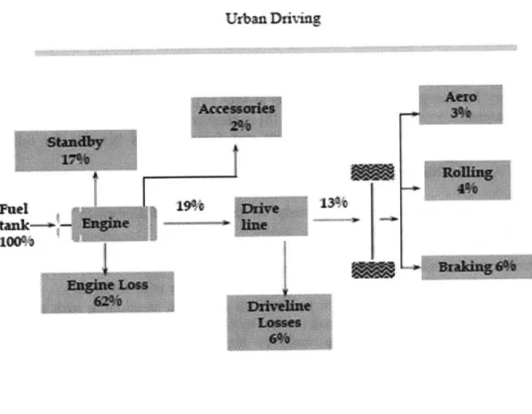
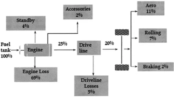
Figures 11 and 12 show typical energy flows for a midsize passenger car during urban and highway driving respectively. They were adapted from [16]. From the initial 100% of the energy in the fuel in the fuel tank only about 13-21% ends up at the wheel actually moving the vehicle. The rest is lost as engine and driveline (transmission) losses, wasted while the engine is idling (standby) or powers accessories. The energy that actually ends up at the wheel is used to overcome aerodynamic and rolling resistances and to accelerate the vehicle. The first two parts of the mechanical energy at the wheel are immediately dissipated as heat. The power used to accelerate is also eventually dissipated as heat when the vehicle decelerates through braking.
There are therefore, two ways in which the fuel consumption of a given vehicle may be reduced:
1. Reducing the amount of energy per distance driven required at the wheel.
2. Improving the average efficiency of the powertrain used to produce and deliver this energy at the wheel. Idling reduction may be viewed as another way of improving engine average efficiency.
Reducing the accessory load would be a third way to reduce fuel consumption. The historical trend however has been that this load has been increasing as more and more gadgets are added to vehicles. The size of auxiliary loads depends more on consumer trends and less on technical improvements. The effect of auxiliaries was therefore neglected throughout this study.
UrbanDdiving i~s Fuel tank- -'100% 13% -*
-Figure 11: Example urban driving energy flows for a late-model midsize passenger car. Source: [16]
Highway Dving
W4
'~ Fuel .tank-
!
ILOO%I
Figure 12: Example highway driving energy flows for a midsize passenger car. Source: [16]
1.7.
Thesis Outline
This thesis consists of six chapters. The scope and methodology of the analysis are introduced to the reader in chapter one. The potential for non powertrain improvements and the assumptions made are analyzed in chapter two. Predictions for different types of internal combustion engines are made in chapter three. Transmission and integration issues are addressed in chapter four. The future of hybrids is discussed in chapter five. The results of the calculations are presented and interpreted in chapter six.
2. Non-Powertrain Improvements
2. 1.Introduction
In this chapter, the potential for reducing the amount of energy a vehicle needs at the wheel will be analyzed. First, the underlying physics that determine the amount of energy per distance driven will be analyzed. This analysis will point out the areas where the opportunities for reducing that energy are. The methodology used to predict how much of this potential will be realized within the time frame of this analysis (25 years into the future) will be subsequently explained for each area.
2.2. Vehicle Resistances
'/
OO
Figure 13: Vehicle moving at a velocity V up a hill. Adapted from [4]
Figure 13 shows a vehicle of mass Mv traveling up a hill of slope a at a velocity V. Newton's second law for the vehicle is:
S*MV d j tj t (2.1)
dt
Where EFt is the total tractive effort of the vehicle , EFtr is the sum of all vehicle resistance forces. 6 is a number larger than one to account for rotating inertias.
As seen on Figure 13, vehicle resistances consist of:
* Rolling resistances: These are presented in the figure in the form of torques Tr, and Tf on the frontal and rear wheels respectively. The total rolling resistance torque can be approximated as:
T, =F, *r, =c, *M,*g*cosa*r, (2.2)
where r, is the wheel radius. The coefficient cr is called the rolling friction coefficient. It depends weakly on vehicle speed but can be assumed constant with good accuracy.
* Aerodynamic force Fw: This is exerted on the center of aerodynamic pressure. It is generally approximated as:
F =I*Pi *C *A*V 2 (2.3) 2
Where pair is the density of the surrounding air, cD is the coefficient of drag which
depends on the vehicle shape and may be assumed independent of speed for the purposes of this analysis, A is the cross-sectional area of the vehicle and Vw is the relative velocity of the wind with respect to the moving vehicle. For no wind conditions, it is the same as the vehicle velocity.
* Grade Resistance. This is apparently zero when driving up a flat road. The general expression is:
Fg = M, * g *sin a (2.4)
* Although it is not theoretically a resistance, the acceleration force should be considered one. It is not a resistance because the power used to accelerate the vehicle is not immediately dissipated as heat, as is the case with the other resistances. It does however increase fuel consumption because:
* The kinetic energy due to the acceleration force is usually lost as heat when the vehicle needs to decelerate through conventional friction
braking.
* Even if the vehicle has regenerative braking capability, this kinetic energy can not be fully recovered as will be explained in chapter four.
As already explained, the acceleration force, Faccei is:
dV Fc =6*M,* *. (2.5)
dt
The relative balance of rolling friction and aerodynamic drag is presented versus vehicle speed for the two baseline vehicles used in this study, the 2.5 liter 2005 Camry and the 4.2 liter F-150 in Figure 14 and Figure 15 respectively. It is obvious that rolling friction dominates at low speeds up to 50-60kmi/h and aerodynamic resistance at higher ones. If a road grade G=tana is additionally imposed on the vehicle, the total resistance force can be seen in Figure 16.
The instantaneous total resistance for the 2005 2.5 liter Camry over the FTP (urban driving) and HWFET (highway) cycles are presented in Figures 17 and 18.It is obvious that acceleration forces dominate urban driving while aerodynamic forces dominate highway resistances. The required energy at the wheel to overcome each resistance can be calculated by integrating the required power over the driving cycle:
E = JPdt = JF*udt (2.6)
drivngcycle drivingcycle
The results from calculating this integral over the two driving cycles are presented in Table 2. Note that in calculating this integral for acceleration, only the negative values of Faccei were included in the calculation of the above integral as that is essentially the energy lost through braking.
Aerodynamic and Rolling Resistance Vs Vehicle Speed for the 2005 2.51t Toyota Camry 203r0 2000 F 1500 -z 1000- 500-0- 50 100 km/h 150 200 250
Figure 14: Aerodynamic and Rolling Resistances versus Vehicle speed For the 2005 2.5 liter Toyota Camry
- Rolling Resistance Force
-Aerodynamic Resistance Force I
Aerodynamic and Rolling Resistance Vs Vehicle Speed for the 2005 4.2 It Ford F1 50 30001 -- rII 25002000 -z 1500- 1000-500 010 km/h
Figure 15 : Aerodynamic and Rolling Resistances versus Vehicle speed for the 2005 F150
Total Vehicle Resistance at the Wheel vs Vehicle Speed and Grade for the 2005 2.5lt Toyota Camry
annnn 8000 -7000 z 6000- 5000- 4000- 3000- 2000-1000 -" 0 50 100 km/h 150 200 4.2 liter Ford - 0% grade --- 5% grade 10% grade 15% grade +20% grade - 25% grade -- '-30% grade --. -35% grade -"40% grade 45% grade 250
Figure 16: Vehicle Resistances Including Grade for the 2005 2.5 liter Toyota Camry. - Aerodynamic Resistance Force
- Rolling Resistances Force
-.
-I I I I
200
50 100 150 250
---Vehicle Resistances over the FTP for the 2005 2.5 liter Camry -Acceleration Force
--- Rolling Friction Force -'-Aerodynamic Force
L
m
ErpriFMI .RR W. - iiiiN"W
time(s)
1500
Figure 17: Vehicle Resistances over the FTP driving Cycle for the 2005 2.5 liter Camry Vehicle Resistances over the HWFET for the 2005 2.5 liter Camry
100 200 300 400
time (s)
500 600 700 800
Figure 18: Vehicle Resistances over the HWFET driving Cycle for the 2005 2.5 liter Camry 3000 2000 1000 z 0 I -1000 -2000 --30000 500 1000 2000 2500 3UU 2000 1000 z 0 -Acceleration Force
-- Aerodynamic Resistance Force --- Rolling Friction Force
I I I I -1000- -2000--3000 I I I
1'
wTable 2: Energy required at the Wheel due to different Resistances
FTP HWFET
% over
% over Total Total
Energy at the Energy at
MJ
Wheel MJ the WheelEnergy to overcome Aerodynamic Drag 1.9 21% 3.6 47% Energy to overcome Rolling Friction 2.5 27% 2.3 30% Braking Energy 4.8 52% 1.8 23%
2.3. Improvements in Vehicle Aerodynamics
High pressure Low pressuremoving direction
Figure 19: Streamlines around a Moving Vehicle
As seen in Figure 19, the flow behind a moving vehicle creates a low-pressure wake. It is mainly this difference of pressures in front of and behind the vehicle created by the flow that causes aerodynamic drag. The effect of size is included in the cross-sectional area A, while the effect of geometry is included in the coefficient of drag, cD in equation
(2.6).
The definition of cross-sectional area is the projected area of a body in the direction
of the flow. It is usually approximated as