HAL Id: hal-02423381
https://hal.archives-ouvertes.fr/hal-02423381
Submitted on 24 Dec 2019HAL is a multi-disciplinary open access archive for the deposit and dissemination of sci-entific research documents, whether they are pub-lished or not. The documents may come from teaching and research institutions in France or abroad, or from public or private research centers.
L’archive ouverte pluridisciplinaire HAL, est destinée au dépôt et à la diffusion de documents scientifiques de niveau recherche, publiés ou non, émanant des établissements d’enseignement et de recherche français ou étrangers, des laboratoires publics ou privés.
To cite this version:
Iskander Abroug, Nizar Abcha, Armelle Jarno, François Marin. Physical modelling of extreme waves: Gaussian wave groups and solitary waves in the nearshore zone. Congrès Françaisde Mécanique 2019, Aug 2019, Brest, France. �hal-02423381�
Physical modelling of extreme waves:
Gaussian wave groups and solitary waves in
the nearshore zone
Iskander ABROUG
a,b, Nizar ABCHA
b,*, Armelle JARNO
a,
François MARIN
aa. LOMC, UMR 6294, CNRS, Normandie Univ, UNILEHAVRE, 76058 Le Havre, France
b. M2C, UMR 6294, CNRS, Normandie Univ, UNICAEN, 14000 Caen, France *nizar.abcha@unicaen.fr
2
Abstract
Laboratory-scale waves of two distinct types were generated in a two- dimensional wave flume to model the spatial evolution of the frequency spectrum in the nearshore zone. The two generated types are Gaussian wave groups of different spectra widths and solitary waves. In the experiment, the time series of free surface elevation along the flume are obtained along a distance of 10m using wave gauges. For each Gaussian wave train, four regions were defined, namely peak, transfer, high frequency and low frequency region referred to as E1, E2, E3 and E4. The repartition was based on the maximum frequency spectrum situated in E1 at X=4m. Focusing is a complex process; this is mainly due to nonlinear energy transfer between different frequency ranges. It was concluded that the energy keeps stable in E1 and spreads toward E3 before breaking. The frequency spectrum in E2 has a decreasing trend during the wave train propagation and this is more appreciable for stronger wave breaking. After the breaking, the frequency spectrum in E2 stops decreasing. It was found also that frequency spectrum increases during the focusing process in E4. Concerning solitary waves, it was found that the frequency spectrum of the main solitary wave decreases as the wave approaches the breaking zone.
Key words: Gaussian wave train/ frequency spectrum/ solitary wave/ peak frequency region/ Transfer region.
Nomenclature
E1, E2, E3 and E4: peak region, transfer region, high frequency region and low frequency region (Gaussian waves).
Es: mains solitary wave frequency region situated between 0.7fp and 1.5fp, where
fp being the peak frequency.
X [m]: Distance along the flume.
A’ [m]: Solitary wave amplitude at the toe of the slope.
A0 [m]: Solitary wave amplitude at X=4m from the wave maker.
Ab [m]: local breaking height.
As [m]: Solitary wave amplitude.
C [m.s-1]: Solitary wave celerity.
3
fp [Hz]: Peak frequency.
fs [Hz]: Characteristic frequency; Eq. 3.
g [m.s-2]: Gravitational acceleration. h [m]: Water depth.
hb [m]: local breaking depth.
k [rad.m-1]: Wave number.
S0: Global wave steepness (at X=4m from the wave maker).
S(f): Frequency spectrum.
Xb [m]: Breaking position.
η (x, t) [m]: Free surface elevation.
Δf [Hz]: Frequency stepping.
φ [rad]: Phase at focusing.
1. Introduction
Giant waves correspond to waves of very high amplitude, appearing mainly on high seas [1]. These waves may be accompanied by deep troughs that may appear before or after the highest peak. The appearance of unusually high waves in the nearshore zone is often associated with the transformation of these waves propagating from the open ocean to the shoreline. The physical processes involved in the transformation of these waves from the open sea to the coastal zone are poorly understood, despite the significant impact these waves may have on the coasts, such as overtopping, material damages, and erosion [2].
These waves can be investigated experimentally using a large variety of physical mechanisms including solitary waves and group focused waves [1]. The first description of solitary waves was made by John Russel [3]. These waves are traditionally used as tsunami approximations because of their hydrodynamic similarity [4]. Group focused waves are often cited in the framework of freak wave formation and have been widely used to study the statistics of rogue waves and their deviation from linear theory [5]. The generation mechanism is defined by the fast spreading of long waves and slow propagation of short waves [6]. The spatial evolution of frequency spectrum of waves in coastal zones is important in assessing danger to life and to marine constructions. However, data are sparse and the phenomenon is hard to investigate, especially in the inner surf zone.
4
Several studies have analysed the spatial evolution of the frequency spectrum of wave trains using the method of energy focusing [7, 8]. Most of these studies were conducted at deep-water conditions. The evolution of the frequency spectrum of group focused waves in intermediate and shallow water depth have received little attention. Rapp and Melville [9] and Tian et al. [10] found that energy loss due to breaking concerns mostly high frequency regions. By making simple comparisons of measurements upstream and downstream the breaking in deep-water depth, Yao and Wu [11] found that the frequency spectrum increases during the wave train propagation in low frequency regions (E4).
Recently, Merkoune et al. [12] reported an experimental study on energy dissipation of non-breaking focused wave groups in the presence of currents. They found that losses are around 25% of the total energy. These losses are caused by viscous dissipation and contact line. Energy calculations are simply based on free surface elevation measurements and not on detailed frequency spectra, even though the focusing process is far from linear superposition. Yao and Wu [11] found that during the propagation, the frequency spectrum in low frequency regions increases. This gain is attributed to losses in high frequency regions, more precisely in first harmonic region.
The paper is organised as follows. Section 2 describes the experimental setup and wave parameters. Section 3 is devoted to the results for Gaussian wave trains and solitary waves. The discussion is presented in section 4.
2. Materiel and methods
2.1. Experimental setup
The experiments were carried out in a wave flume of the coastal and continental morphodynamics Laboratory at Caen University, France. The flume is 20m long and 0.8m wide. An Edinburgh designs Ltd piston-type paddle was used to generate waves propagating through 0.3 m depth to a sloping bottom of an angle β=0.04 rad situated at X=9.5m downstream the wave maker (Fig. 1). The flume bottom is elevated 1.15m from the ground to ease side visualisations. The governing parameters include the initial solitary wave amplitude A0 (S0 is the input steepness
for Gaussian wave trains), the free surface elevation η (x, t), breaking location Xb
5
Figure 1: Experimental setup
The free surface elevations were recorded at different locations along the flume with resistive wave gauges. The first gauge is fixed and used as a temporal reference, the second gauge is moved 20 cm after each test (Fig. 1). Free surface elevations are overlaid chronologically at regular time intervals in order to obtain space-time diagrams. The fast Fourier transformation (called FFT) is computed for each signal measured by the wave gauges using Matlab [13, 14]. Additional video tests have been conducted to track the breaking process with a camera, which was set to record at a frequency of 100Hz. Each experiment requires a time interval of 5 minutes to ensure that the water surface is calm. For group focused waves, the input focusing point was fixed on X=12m in order to have a focusing on the slope.
6
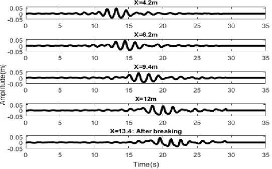
It is important to clarify that the breaking on the slope will prevent complete focusing. Thus, the focusing is not experimentally perfect and so only breaking locations are mentioned in Table 1. Figure 2 presents time histories of the measured free surface elevation of a Gaussian wave train (GW2) at five locations.
2.2. Wave parameters
Gaussian wave trains are generated using dispersive focusing technique. In this experiment, we adopted the Gaussian distribution to generate breaking waves in shallow water using wave energy focusing. According to linear theory, the free surface elevation can be written as follows:
𝜂(𝑥, 𝑡) = ∑𝑛𝑖=1𝑎𝑖cos(𝑘𝑖𝑥 − 𝜔𝑖𝑡 + 𝜑𝑖) (1)
A wave train contains a range of individual linear sine wave components, each with amplitude ai, angular frequency ωi and wave number ki. The phase angle
of each component φi was adjusted so that the crests of the individual components
coincide at a selected location and time. We assume that the discrete frequency fi
(ωi/2π) is uniformly distributed between f1 and f2. Therefore, the frequency width
and center frequency are defined by:
Δf=f2-f1; fc= 0.5*(f1+f2) (2)
Four different bandwidths (i.e. Δf/fc) were set in order to investigate the
variation of this parameter. The spectrally weighted frequency (fs) is chosen as the
characteristic frequency of the wave train and is calculated using equation (3) [10]. 𝑓𝑠 =∑ [𝑓𝑖𝑎𝑖
2 𝑛
𝑖=1 (𝛥𝑓)𝑖]
∑𝑖𝑖=1[𝑎𝑖2(𝛥𝑓)𝑖] (3)
Here, fi is the frequency of the ith component of the wave packet and Δfi is
the difference between components, which is constant. Unlike solitary waves, wave group’s nonlinearity cannot be characterised by a single amplitude, and therefore global wave steepness is used. Equation (4) given in [10] was chosen to calculate this parameter through spectrum analysis of wave gauge data at X=4m.
𝑆0 = 𝑘𝑠∑𝑛𝑖=1𝑎𝑖 (4)
Here, ks is the spectrally weighted wavenumber related to fs and ∑𝑛𝑖=1𝑎𝑖is
the surface elevation at the focusing point according to linear wave theory. With working depth h=0.3m, the value of kch is calculated using the finite depth
dispersion relation. Hence, wave trains start propagating in intermediate water depth (i.e. kch=0.93) to coastal zones. Each measurement is decomposed into 90
7
Fourier components and the correspondent surface elevation is expressed analytically as a summation of sinusoidal waves in order to determine different amplitudes (ai) and frequencies (fi) (Equation (5)) [15].
𝐹(𝑓) = ∫ 𝜂(𝑡)𝑒𝑇 −2𝜋𝑖𝑓𝑡𝑑𝑡
0 (5)
Here, F(f) is the Fourier transform of η(t) in a given location, T is the signal duration and is equal to 35s in our study (the time stepping is 0.02s). Careful observation of the free surface elevation shows that the signal duration is sufficient since it includes all meaningful wave components. The wave frequency spectrum is calculated as𝑆(𝑓) = 2|𝐹(𝑓)|2/𝑁 where N is the number of points corresponding
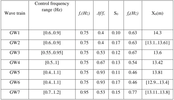
to the sampling time. For present tests, N=35/0.02=1750 points Table 1: Gaussian wave trains parameters
Wave train Control frequency range (Hz) fc(Hz) Δf/fc S0 fp(Hz) Xb(m) GW1 [0.6..0.9] 0.75 0.4 0.10 0.63 14.3 GW2 [0.6..0.9] 0.75 0.4 0.17 0.63 [13.1..13.61] GW3 [0.55..0.95] 0.75 0.53 0.12 0.67 13.6 GW4 [0.5..1] 0.75 0.67 0.13 0.54 13.42 GW5 [0.4..1.1] 0.75 0.93 0.11 0.46 13.81 GW6 [0.4..1.1] 0.75 0.93 0.17 0.46 [12.9...13.4] GW7 [0.7..1.2] 0.95 0.53 0.15 0.77 [13.11..13.8]
Boussinesq derived a mathematical expression for the solitary wave profile generated on a horizontal, rectangular channel [16]. Equation (6) indicates the nonlinear solution obtained by Boussinesq approximation [17].
8
Here, As is the solitary wave amplitude, V the theoretical wave velocity, x
is the horizontal distance and t isthe time.
C is the wave celerity given by:
𝐶 = √𝑔(ℎ + 𝐴𝑠) (7)
Figure 3 shows a comparison between the experimental time history of the free surface elevation and the time history predicted by Equation (6) at X=4m downstream the wave maker. One can observe an excellent agreement between the experimental and the theoretical solution. In the generation of solitary waves, small trailing waves due to the piston pullback are observed behind the main solitary wave.
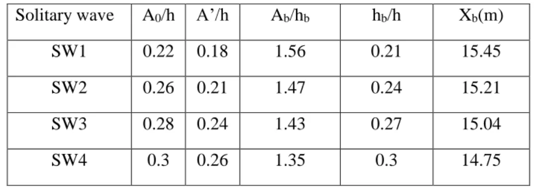
Table 2: Solitary waves parameters
Solitary wave A0/h A’/h Ab/hb hb/h Xb(m)
SW1 0.22 0.18 1.56 0.21 15.45 SW2 0.26 0.21 1.47 0.24 15.21 SW3 0.28 0.24 1.43 0.27 15.04 SW4 0.3 0.26 1.35 0.3 14.75
Table 1 indicates the different parameters corresponding to the seven Gaussian wave trains and Table 2 presents the parameters for the four solitary waves generated during the physical experiments.
Figure 3: The measured water surface elevation compared to the Boussinesq solitary
9
3. Results
3.1. Gaussian wave trains
3.1.1. The frequency regions
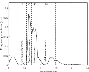
To distinguish between different frequency regions, a repartition has been performed on the initial spectrum S0(f) at X=4m.
E1, E2, E3 and E4 are respectively peak, transfer, high frequency and low frequency regions. These four different frequency regions are illustrated in Figure 4.
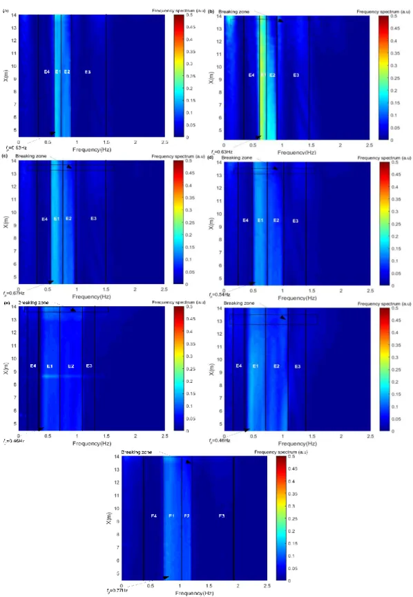
Figure 5 shows spectrograms of the seven wave trains. These plots
represent the frequency spectrum evolution during the wave train propagation. As mentioned above, different distributions have been performed on all spectra since their shapes differ. It should be noted that the repartition was based on the maximum frequency spectrum situated in E1 at X=4m. The lower limit for E4 is 0.6fp and the
upper limit corresponds to 10% of the maximum frequency spectrum. The peak frequency region limits are different from one spectrum to another (Fig. 4). The lower and the upper limits have been selected in order to guarantee that all significant frequency spectra around the peak frequency are considered. The transition to E2 is characterised by a decrease of 60% of the maximum frequency spectrum. The upper limit of E2 coincides with 20% of the maximum frequency spectrum. Subsequently, E3 is situated beyond E2. The upper limit was chosen to be equal to 2.5fp. The spectral energy beyond this region is less than 3% of the total
frequency spectrum and can be neglected.
Figure 4: Typical repartition of the initial spectrum S0(f) for GW1
10
Figure 5: Spectrograms as obtained by wave gauges through FFT (a) GW1, (b): GW2, (c): GW3, (d): GW4, (e): GW5, (f): GW6, (g): GW7. The colorbar indicates the wave
11 3.1.2. Spatial evolution of the frequency spectrum
In this section, all energy forms are normalized by E0, which is the integral of the wave frequency spectrum S(f) between cut-off frequencies 0.6fp and 2.5fp
Energy variations are quantified as a function of space by integrating the wave frequency spectrum obtained at every 20cm from X=4m up to X=14m.
The initial frequency spectrum in E1 is between 45% and 60% of the total frequency spectrum. Figure 6 shows that the frequency spectrum in E1 increases slightly on the flat bottom (4m<X <9.5m) for all studied wave trains. Thus, it increases by 8% of its initial level for GW2. After breaking, the spectral energy in E1 decreases for the case of GW2 and GW7 and eventually reaches around 90% of their initial levels. This decrease is primarily caused by dissipation and nonlinear energy transfer to higher frequency regions [10].
The frequency spectrum in the transfer region (E2) decreases gradually and significantly upstream breaking. This behaviour is similar for all steepness and for all bandwidths of the studied wave trains. After the breaking, the frequency spectrum in E2 stops decreasing and begins to recover. For the two Gaussian wave trains having the same frequency bandwidth (GW1 and GW2), the frequency spectrum decrease in E2 is more obvious for GW2 when compared to GW1. This is more clear for wider wave trains (GW5 and GW6). The frequency spectrum in E2 for GW5 reaches around 85% of its initial level after breaking and for GW6 it reaches around 50% of its initial level after breaking. The frequency spectrum loss in E2 for the two Gaussian wave trains with approximately the same steepness (WG2 and GW6) is approximately the same.
The frequency spectrum in high frequency region (E3) increases gradually during the wave train propagation. For instance, it reaches 30% of its initial level for GW2 at the toe of the slope. The observed energy transfer from the first harmonic to higher harmonics is consistent with earlier studies in [10, 13]. Therefore, the energy transfer is similar to that in deep water regions. When the wave train breaks, frequency spectrum stops increasing in this region and starts to decrease. This is more obvious for GW2 and GW7. This can be explained by the reversibility of the nonlinear energy transfer between E2 and E3 [15].
In lower frequency region (E4), the spectral energy increases during the wave train propagation for the seven studied wave trains. This is consistent with [9, 10]. A possible nonlinear energy transfer from E2 and E1 to E4 could offer an explanation
12
Figure 6: Spatial evolution of frequency spectrum for (a): GW1, (b): GW2, (c): GW3, (d): GW4, (e): GW5, (f): GW6, (g): GW7. ■ frequency spectrum in E1; ● frequency spectrum in
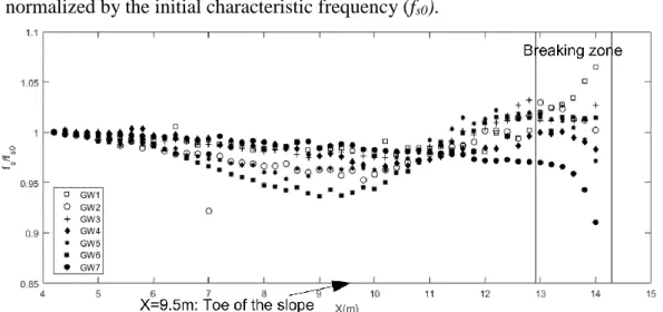
13 3.1.3. Characteristic frequency
The characteristic frequency is a good predictor of energy transfer and frequency spectrum changes during the focused wave group propagation [18]. According to Equation (3), fs is sensitive to energy transfers as long as all the
meaningful frequency components are included in its determination. Fourier frequency components in the range of [0.6fp, 2.5fp] Hz are included in the
calculation of fs. The characteristic frequency is determined at X=4m and is
normalized by the initial characteristic frequency (fs0).
Figure 7 shows the spatial evolution of spectrally weighted frequency. Two vertical solid lines are plotted in the same figure in order to indicate the breaking regions for different wave trains. It is found that fs is stable from X=4m to X=5.5m.
On the flat bottom, the characteristic frequency decreases gradually for all Gaussian wave trains, which is more obvious for wide spectrum waves. This decrease is explained by energy dissipation in E1 and E2. Just prior to breaking, fs increases
slightly and this is mainly due to spreading in high frequencies and to spectrum broadening. When the wave train breaks, fs decreases, indicating a decreasing trend
in high frequency regions. The characteristic frequency almost returns to its initial value after breaking. However, it does not recover to its initial value for the two weakest wave trains (GW1 and GW3) since they break at X>13.5m.
14
3.2. Solitary wave
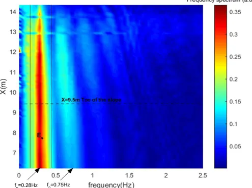
Figure 8 presents the spectrogram for SW4, on which the narrow band at
f=0.28Hz (Es) corresponds to the spatial evolution of the frequency spectrum of the
solitary wave. One can see a second band at approximately 0.75 Hz, which corresponds to the frequency spectrum of the wave generated by the piston pullback. In terms of frequency spectrum, this band and the following bands of higher frequencies (1 Hz and 1.25 Hz) are less intense than the main band (0.28 Hz). Higher frequency waves travel slower than lower frequency waves and reach the shore after the solitary wave [19]. Therefore, high frequency waves do not have a significant impact on the spatial evolution of the main solitary wave. Furthermore, the band at approximately 0.15Hz corresponds to low frequency waves. These subharmonic waves are present along the flume and are amplified by shoaling when arriving on the slope. However, they are approximately three times less energetic than the main solitary wave. Hence, we consider that the subharmonic wave effect is not significant.
Figure 8: Spectrogram of SW2 as obtained by wave gauges through FFT. The colorbar indicates the wave frequency spectrum S(f)
15
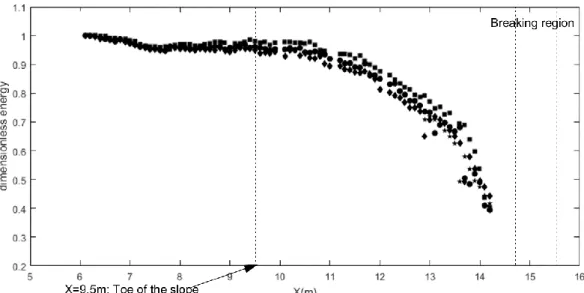
The frequency spectrum of the main solitary wave is mainly situated between 0.7fp and 1.5fp. Figure 9 shows that the frequency spectrum in Es decreases
gradually on the flat bottom (4m<X<9.5). It is important to clarify at this point that the decrease rate slightly depends on the initial solitary wave steepness (A0). The
frequency spectrum reaches around 97% of its initial level for SW1 and around 93% of its initial level for SW4 at X=9.5m from the wave maker. This decrease is intensified when the solitary wave reaches the slope and is explained by the shoaling phenomenon, which has an impact on the solitary wave shape. This can be seen clearly by the narrowing of the solitary wave spectrum in Figure 8. For instance, this energetic decline reaches around 40% of its initial level for SW2. We can conclude from Figure 9 that the frequency spectrum loss is slightly impacted by the initial solitary wave steepness and the decreasing rate on the sloping bottom is fairly similar for the four solitary waves.
4. Discussion
This paper describes the spatial evolution of Gaussian wave groups and solitary waves along a flat and sloping bottom using a series of physical experiments. Different breaking intensities, center frequencies and frequency widths are considered for Gaussian wave trains. The spatial evolution of frequency spectrum upstream and downstream the wave breaking is studied for each test, thanks to 50 measurements carried out by wave gauges.
Figure 9: ■ spatial evolution of frequency spectrum for SW1; ● SW2; ★ SW3; ♦ SW4
16
On the one hand, four energy regions are defined with the aim of monitoring the spatial evolution of frequency spectrum upstream and downstream the breaking for Gaussian wave trains. The repartition was based on the maximum frequency spectrum at X=4m. It was found that the energetic behavior is relatively similar for the seven generated wave trains and this confirms the limits that were defined. On the other hand, solitary waves are only described by one frequency region.
Based on our experimental data, the energy dissipation for solitary waves on the flat bottom (4m<X <9.5m) is small. For the steepest solitary wave, the energy dissipation is around 10%. These losses are caused by viscous dissipation and contact-line damping. Concerning Gaussian wave trains, the total energy dissipation is insignificant on the flat bottom and is around 8% for the strongest wave train GW7. The total energy keeps stable along the 5.5m for the weakest wave trains and this is consistent with earlier studies in [18]. It should be mentioned that in our experiments losses of energy are smaller than in [12]. This difference found in [12] can be explained by the larger influence of viscose boundary layers at sidewalls and on the bottom since our measurements are performed at larger flume width.
On the sloping bottom (9.5m<X <Xb), the shoaling happens. The energy
behaviour differs for the two wave types. In fact, the main solitary wave is marked by a strong energy decrease. For Gaussian wave trains; however, the energetic increase in higher harmonic regions (E3) and the energetic decrease in the transfer region (E2) are intensified which indicates a stronger energy transfer than that on the flat bottom.
Along the wave train propagation, the energy decreases in higher frequencies of the controlling frequencies range and increases slightly in the peak region.When the wave trains breaks, the frequency spectrum increase in E3 ceases and begins to decrease. This is consistent with earlier studies [13, 18]. Thus, the behaviour of spectral energy in E2 and E3 in intermediate and shallow water depth is close to that in deep water depth.
For the near future, we plan to perform new tests involving other spectra such as Pierson-Moskowitz and JONSWAP spectrum, in order to extend our experimental results to more realistic spectra.
Acknowledgments
17
References
[1] C. Kharif, E. Pelinovsky, Physical mechanisms of the rogue wave phenomenon, in: European Journal of Mechanics B, 2003, 22, 603-635.
[2] A. Strusińska-Correia, H. Oumeraci, Nonlinear behavior of Tsunami-Like solitary wave over submerged impermeable structures of finite width, in: Coastal engineering proceedings, 2012, icce. v33. Currents.6
[3] J. S. Russel, Report on waves, in: Proceedings. 14th Meeting. Brit. Ass. Adv, 1845. Pp. 311-390.
[4] S. C. Hsiao, T. C. Lin, Tsunami-like solitary waves impinging and overtopping an impermeable seawall: Experiment and RANS modeling, in: Journal of Coastal Engineering, 2010, Volume 57 , Issue 1, Pages 1-18.
[5] N. Mori, M. Onorato, P. A. E. M. Janssen, A. R. Osborne and M. Serio, On the extreme statistics of long-crested deep-water waves: Theory and experiments in: Journal of Geophysical Research, 2007, 112, C09011.
[6] J. Touboul, E. Pelinovsky, C. Kharif, Nonlinear focusing wave group on current, in: Journal of Korean Society of Coastal and Ocean Engineers, 2006, 19, 222-227. [7] T. Johannessen, C. Swan, a laboratory study of the focusing and transient and directionally spread surface water waves, in: Proceedings of the Royal Society A, London: Math. Phys. Eng. Sci, 2001, 457, 971-1006.
[8] M. L. Banner, W. L. Peirson, Wave breaking onset and strength for two-dimensional deep-water wave groups, in: Journal of Fluid mechanics, 2007, 585:93-115.
[9] R. Rapp, K. W. Melville, Laboratory measurements of deep-water breaking waves in: Philosophical Transactions of the Royal Society A, London, 1990, A. 331, 735-800.
[10] Z. Tian, M. Perlin, W. Choi, Frequency spectra evolution of two dimensional focusing wave groups in finite water depth water, in Journal of Fluid Mechanics, 2011, vol. 688, pp. 169-194.
[11] A. F. Yao, C. H. Wu, Energy dissipation of unsteady wave breaking on currents, in: Physical. Oceanography, 2004, 34, 2288-2304.
18
[12] D. Merkoune, J. Touboul, N. Abcha, D. Mouazé, A. Ezersky, Focusing wave group on a current of finite depth, in: Natural hazards and earth system sciences, 2013, Sci., 13, 2941-2949.
[13] T. Baldock, T.E. Swan, P. H. Taylor, A laboratory study of non-linear surface waves on water, in: Philosophical Transactions of the Royal Society A. R. Soc. London, Ser, 1996, A, 354, 1-28 5.
[14] R. S. Gibson, C. Swan, The evolution of large ocean wave: The role of local and rapid spectral changes, in: Proceedings of the Royal Society A, London, Ser, 2007, A, 463-2077-21-48.
[15] Z. G. Tian, M. Perlin, W. Choi, energy dissipation in two-dimensional unsteady plunging breakers and an eddy viscosity model, in: Journal of Fluid Mechanics, 2010. 655, 217-257.
[16] M. H. Boussinesq, Théorie de l’intumescence liquide, appelée onde solitaire ou de translation, se propageant dans un canal rectangulaire, C.-R. Acad. Sci. Paris, 1871, 72p.
[17] D. D. Goring, Tsunami-the propagation of long waves onto a shelf, in: PhD thesis, 1979, California Institute of Technology, Pasadena, Calif.
[18] S. Liang, Y. Zhang, Z. Sun, Y. Chang, Laboratory study on the evolution of waves parameters due to wave breaking in deep water, in: Wave motion, Volume 68, 2017, Pages 31-42.
[19] J. Orszaghova, H. P. Taylor, G. L. Alistair, Borthwick, A. C. Raby, Importance of second-order wave generation for focused wave group run-up and overtopping, in: Journal of Coastal Engineering, 2014, 94, 63-97
List of figures
Figure 1: Experimental setup ... 5 Figure 2: Free surface elevation as measured by wave gauges of GW2 ... 5 Figure 3: The measured water surface elevation compared to the Boussinesq solitary wave of the same maximum height ... 6 Figure 4: Typical repartition of the initial spectrum S0(f) for GW1... 6
19
Figure 5: Spectrograms as obtained by wave gauges through FFT (a) GW1, (b): GW2, (c): GW3, (d): GW4, (e): GW5, (f): GW6, (g): GW7. The colorbar indicates the wave frequency spectrum S(f) (arbitrary units) from X=4m to
X=14m ... 6 Figure 6: Spatial evolution of frequency spectrum for (a): GW1, (b): GW2, (c): GW3, (d): GW4, (e): GW5, (f): GW6, (g): GW7. ■ frequency spectrum in E1; ● frequency spectrum in E2; ★ frequency spectrum in E3; ♦ frequency spectrum in E4 ... 6 Figure 7: Characteristic frequency spatial evolution ... 6 Figure 8: Spectrogram of SW2 as obtained by wave gauges through FFT. The colorbar indicates the wave frequency spectrum S(f) (arbitrary units) from X=4m to X=14m ... 6 Figure 9: ■ spatial evolution of frequency spectrum for SW1; ● SW2; ★ SW3; ♦ SW4 ... 6