December 2008
Plasma Science and Fusion Center Massachusetts Institute of Technology
Cambridge MA 02139 USA
This work was supported by the U.S. Department of Energy, Grant No. DE-FC02-99ER545512. Reproduction, translation, publication, use and disposal, in whole or in part, by or for the United States government is permitted.
PSFC/RR-08-10 DOE/ET-54512-363
Axisymmetric Equilibrium and Stability Analysis in
Alcator C-Mod, Including Effects of Current Profile,
Measurement Noise and Power Supply Saturation
Axisymmetric Equilibrium and Stability Analysis in
Alcator C-Mod, Including Effects of Current Profile,
Measurement Noise and Power Supply Saturation
by
Marco Ferrara
S.M. Nuclear Science and Engineering (2005)
Submitted to the Department of Nuclear Science and Engineering
in partial fulfillment of the requirements for the degree of
Doctor of Philosophy
at the
MASSACHUSETTS INSTITUTE OF TECHNOLOGY
February 2009
c
° Massachusetts Institute of Technology 2009
The author hereby grants to Massachusetts Institute of Technology
permission to reproduce and
to distribute copies of this thesis document in whole or in part.
Signature of Author . . . .
Department of Nuclear Science and Engineering
December 3, 2008
Certified by. . . .
Ian H. Hutchinson
Department Head, Nuclear Science and Engineering
Thesis Supervisor
Certified by. . . .
Stephen M. Wolfe
Principal Research Scientist, Alcator Project
Thesis Supervisor
Axisymmetric Equilibrium and Stability Analysis in Alcator
C-Mod, Including Effects of Current Profile, Measurement
Noise and Power Supply Saturation
by
Marco Ferrara
Submitted to the Department of Nuclear Science and Engineering on December 3, 2008, in partial fulfillment of the
requirements for the degree of Doctor of Philosophy
Abstract
The vertical position of elongated tokamak plasmas is unstable on the time scale of the eddy currents in the axisymmetric conducting structures. In the absence of feedback control, the plasma would drift vertically and quench on the wall, a situation known as Vertical Displacement Event (VDE), with serious consequences for machine integrity. As tokamaks approach reactor regimes, VDE’s cannot be tolerated: vertical feedback control must be robust against system uncertainty and the occurrence of noise and dis-turbances. At the same time, adaptive routines should be in place to handle unexpected events. The problem of robust control of the vertical position can be formulated in terms of identifying which variables affect vertical stability and which ones are not directly controlled/controllable; identifying the physical region of these variables, and the cor-responding most unstable equilibria; and designing the control system to stabilize all equilibria with sufficient margin. The margin should be enough to allow the system to tolerate realistic scenarios of noise and disturbances. A set of metrics is introduced to characterize the problem of vertical stability: the stability margin describes the plasma-wall interaction and the open-loop growth rate; the maximum controllable displacement looks at the vertical stabilization power supplies and their ability to handle noise and off-normal events; the gain and phase margins quantify the linear stability of the feed-back control loop. The dependence of these metrics on relevant plasma parameters is proven with analytic calculations and numerical simulations: in particular, it is shown that the stability margin is a decreasing function of the plasma internal inductance, for a given plasma elongation. An upper bound of the value of the internal inductance is derived and validated with database analysis, which describes the most unstable equilib-rium for given values of the external elongation and the edge safety factor. The stability metrics are evaluated for typical and ITER-like C-Mod plasmas to give an example of
the C-Mod operational space and of feasible control conditions. The vertical stabiliza-tion system should be able to tolerate realistic scenarios of noise and disturbances. The main sources of noise and pick-ups in Alcator C-Mod are identified and their effects on the measurement and control of the vertical position are evaluated. Broadband noise may affect controllability of C-Mod plasmas at limit elongations and may become an issue with high-order controllers, therefore two applications of Kalman filters are inves-tigated. A Kalman filter is compared to a state observer based on the pseudo-inverse of the measurement matrix and proves to be a better candidate for state reconstruc-tion for vertical stabilizareconstruc-tion, provided adequate models of the system, the inputs, the intrinsic and measurement noise and an adequate set of diagnostic measurements are available. A single-input single-output application of the filter for the vertical observer rejects high frequency noise without destabilizing high-elongation plasmas, however does not match the performance of an optimized low-pass filter. Aggressive control targets and large off-normal events can cause a control current to rail. The magnetic topology is consequently perturbed and the plasma might become uncontrollable. An adaptive anti-saturation control routine is demonstrated which avoids an impending saturation by interpolating in real-time to a safe equilibrium. This approach becomes necessary when poor redundancy of control coils may require mid-shot pulse rescheduling, as opposed to an adaptation in control.
Thesis Supervisor: Ian H. Hutchinson
Title: Department Head, Nuclear Science and Engineering Thesis Supervisor: Stephen M. Wolfe
Acknowledgements
My five years at MIT were an exciting time of professional and personal growth. This would have not been possible without the generous support of the Plasma Science and Fusion Center, for which I’m truly grateful.
I would like to express my admiration for Prof. Hutchinson and Dr. Wolfe for their guidance and trust during my years at MIT, and for Mr. Stillerman for his essential help during my research.
I would like to thank my friends Markus, Jose, Jennifer, Lorenzo, Francesca, Karin, Alessio, Eduardo, Usman for their affection and support; my brother Luca, for being a constant example; and my parents, for providing the solid foundations on which I’ve built.
Contents
1 Introduction 15
2 Linear Model of the Plasma Vertical Position. Stability Metrics 22
2.1 Equilibrium and Stability of a Filament Plasma . . . 22
2.2 Circuit Equations . . . 25
2.3 Plasma-wall Interaction. Stability Margin . . . 29
2.3.1 Plasma Inductance and Stability Margin . . . 31
2.4 Maximum Controllable Displacement. Gain and Phase Margins . . . 34
2.5 Alcasim Simulator . . . 35
2.6 Conclusions . . . 39
3 Plasma Inductance and Stability Metrics on Alcator C-Mod 40 3.1 Physical Space of the Plasma Internal Inductance . . . 40
3.2 Stability Metrics on Alcator C-Mod . . . 46
3.2.1 Experimental Measurement of the Maximum Controllable Displace-ment . . . 56
3.3 Conclusions . . . 60
4 Noise and Pick-ups in Alcator C-Mod 61 4.1 Measurement of Noise and Pick-ups in Alcator C-Mod . . . 61
5 State Observer for Vertical Stabilization Based on a Kalman Filter 70
5.1 System Model Reduction . . . 71
5.2 Kalman Filter Equations . . . 78
5.3 Simulated Behavior of the Filter . . . 80
5.4 Conclusions . . . 95
6 Model-based Filter for the Vertical Observer Based on a Kalman Filter 97 6.1 SISO Filter Equations . . . 97
6.2 Experimental Results . . . 105
6.3 Conclusions . . . 106
7 Current Saturation Avoidance with Real-time Control using DPCS 108 7.1 Anti-saturation Adaptive Control Routine . . . 109
7.2 Multi-processor Multi-timescale Control Scheme . . . 113
7.3 Experimental Results . . . 117
7.4 Conclusions . . . 119
8 Conclusions 121 9 Appendix A. Inductance of a Uniform-current Ellipse 125 10 Appendix B. Chopper Power Supply 127 10.1 Simulation of the Chopper . . . 129
11 Appendix C. DFT Algorithm 132
12 Appendix D. Schur Balanced Truncation 134
13 Appendix E. Linear Model of the Plant 139
List of Figures
1-1 Cross-section of Alcator C-Mod. . . 16 1-2 Flux loops (left panel) and poloidal pick-up coils (right panel) in Alcator
C-Mod. . . 17 1-3 Simplified schematic of the C-Mod feedback control system. . . 18 2-1 Reference coordinate system. The toroidal angle ϕ selects a poloidal plane.
A point in the poloidal plane is uniquely identified by the Cartesian coordi-nates based in the center of the torus (R, z) or by the poloidal coordicoordi-nates based in the geometric center of the plasma cross section (r, ϑ). . . 23 2-2 Magnetic surfaces produced by the superposition of quadrupole field,
ver-tical field and filament plasma. The intensity of the currents is arbitrary. 26 2-3 External field in the example in figure 2-2. . . 26 2-4 Eigenvalue of the plasma-wall mode as a function of the magnetic curvature
index. . . 30 2-5 Top-hat current profile with elongation κ. . . 31 2-6 Stability margin as a function of the internal inductance calculated from
the top-hat plasma model. . . 33 2-7 Simulink model of Alcator C-Mod. The blocks 60HzEF2L, AlternatorEF1U
and AlternatorOH2U model the pick-ups at the output of the power sup-plies connected to the corresponding coils. . . 36
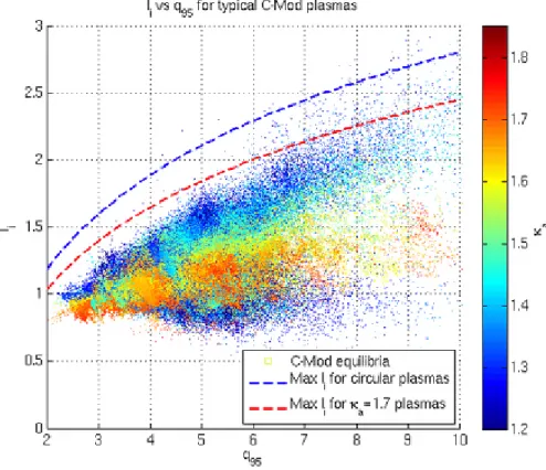
2-8 The passive structures and the active coils are modeled by discrete axisym-metric conducting elements. The plasma is modeled by eight filaments simmetrically located on a current surface. . . 37 3-1 Scatter plot of li vs q95 from equilibria of non-disrupting C-Mod plasmas.
The color is the time during the discharge. The dotted curves are maxi-mum allowable values of li calculated from equation 3.4. . . 42
3-2 Scatter plot of li vs q95 from equilibria of non-disrupting C-Mod plasmas.
The color is the elongation of these equilibria. The dotted curves are maximum allowable values of li calculated from equation 3.4. . . 43
3-3 Scatter plot of li vs κa from equilibria of non-disrupting C-Mod plasmas.
The color is the time during the discharge. The dotted curves are maxi-mum allowable values of li calculated from equation 3.4. . . 44
3-4 Scatter plot of li vs κa from equilibria of non-disrupting C-Mod plasmas.
The color is the safety factor q95 of these equilibria. The dotted curves are
maximum allowable values of li calculated from equation 3.4. . . 45
3-5 The stability margin ms of ITER-q95 plasmas plotted against li. The
vertical error bars are the uncertainty of the linear model used to calculate ms. The horizontal error bar is the uncertainty of the reconstructed li. . 47
3-6 The stability margin ms of C-Mod typical plasmas plotted against li. . . 50
3-7 The stability margin ms calculated for shot 1070406015 as a function of
κa. The observed C-Mod control limit is ms ' 0.26, everything below is
closed-loop unstable. . . 52 3-8 Linearized model of the vertical control loop. The fast ZCUR controller
stabilizes the vertical position of the plasma and is mostly derivative. The slow ZCUR controller controls the vertical position of the plasma and is mostly proportional and integral. . . 53
3-9 Bode plots for four target elongations. The low frequency phase response is shifted by 90 deg because the plasma responds primarily to the time derivative of the magnetic flux. The upward bend starting at 20Hz is largely determined by the fast derivative controller. The frequencies of zero-phase crossing are thus moved away from the frequencies where the magnitude is close to unity, and the feedback loop is stabilized. . . 54 3-10 Details of Bode plots. . . 55 3-11 Vertical position, chopper demand and chopper current during the δzmax
experiment 1071211017. The control gains are zeroed at 0.8s when κa =
1.72. The initial perturbation of the plasma vertical position is small and the plasma drifts only ∼ 7mm by the time the proportional gain is back on at 0.808s. . . 57 3-12 Vertical position, chopper demand and chopper current during the δzmax
experiment 1071211016. The control gains are zeroed at 0.8s when κa =
1.72. There are large oscillations starting at 0.805s when the proportional gain is back on. From the last cycle before disruption it is possible to conclude that δzmax ∼ 28mm at this elongation. . . 58
3-13 Comparison of the maximum vertical displacement in experiments and simulations. . . 59 4-1 Sources of noise and pick-up in Alcator C-Mod. The main sources of noise
are indicated in red: the current noise of the power supplies, the white noise of the magnetic diagnostics and the plasma noise. The main pick-ups are indicated in blue: the alternator and line frequency at the power supplies and the line frequency in the magnetic diagnostics. The chopper bang-bang behavior is mostly negligible because of its high frequency. . . 62 4-2 Comparison of ZCUR power spectra during power supply test shots. . . . 65
4-4 Broadband noise level in the vertical observer as a function of the plasma elongation. . . 68 4-5 PSD of the digital derivative of ZCUR for two different plasmas. . . 69 5-1 Error bound of the Schur balanced truncation of the stable part of a
high-elongation equilibrium as a function of the number of modes retained in the model. . . 73 5-2 Eigenvalues of the reduced model of the stable part of the system for
Nred= 1, 2, 3, 5, 9. The eigenvalues of the model of order 5 are labeled for
future reference. . . 74 5-3 Magnetic flux surfaces of the stable EFC mode. The amplitude of the
eigenmode is normalized. . . 76 5-4 Magnetic flux surfaces of the unstable vertical mode. The amplitude of
the eigenmode is normalized. . . 77 5-5 The linear model used to test the behavior of the Kalman filter. The red
path shows the vertical stabilization loop. The blue path shows the section of the Kalman filter. The green path shows the section of a simple pseudo-inverse state observer used to benchmark the behavior of the Kalman filter. The blocks labeled K*u perform matrix multiplications. . . 81 5-6 Comparison of the real and reconstructed unstable state for different values
of α2. Amplitudes are normalized by the amplitude of the real state. All noise sources where turned off for this test. . . 84 5-7 Comparison of the linear observer and the vertical position calculated from
the reconstructed states for different values of α2. Amplitudes are
normal-ized by the amplitude of the linear observer. All noise sources where turned off for this test. . . 85 5-8 Comparison of real (red) and reconstructed states (blue). Vertical axes
are Amperes. The 54Hz pick-up is off. The model of intrinsic noise is uniform with α2 = 4. . . 87
5-9 RMS value of the error signals between real and reconstructed states. The 54Hz pick-up is off. The model of intrinsic noise is uniform with α2 = 4. 88 5-10 Both the Kalman filter and the pseudo-inverse observer allow a
represen-tation of the vertical position with lower noise than the C-Mod vertical observer. . . 89 5-11 Comparison of real (red) and reconstructed states (blue). Vertical axes
are Amperes. The 54Hz pick-up is off. The model of intrinsic noise is non-uniform with α2 = [4, 4, 4, 64, 64, 4]. . . 90 5-12 RMS value of the error signals between real and reconstructed states. The
54Hz pick-up is off. The model of intrinsic noise is non-uniform with α2 = [4, 4, 4, 64, 64, 4]. . . . 91
5-13 Comparison of real (red) and reconstructed states (blue). Vertical axes are Amperes. The 54Hz pick-up is on. The model of intrinsic noise is non-uniform with α2 = [4, 4, 4, 64, 64, 4]. . . 93 5-14 RMS value of the error signals between real and reconstructed states. The
54Hz pick-up is on. The model of intrinsic noise is non-uniform with α2 = [4, 4, 4, 64, 64, 4]. . . . 94
6-1 Frequency response of the filter for different orders of the reduced model. In this example D = 6, P = 4, α2 = 4. . . 100
6-2 Frequency response of the filter for different values of the noise ratio α2. Solid lines show the analytic transfer function, diamonds are the frequency response calculated from the time traces of Alcasim simulations. . . 101 6-3 Frequency response of the system term FSY S for different values of the
noise ratio α2. . . 102 6-4 Frequency response of the PD controller FCT RL. . . 103
6-6 Comparison of analytic and experimental transfer functions. Diamonds are experimental results from shot 1080430020, where the filter was operating off-line. The gain of the chopper used in the linear model of the filter was 200 and the noise ratio was set to a large value α2 = 16. . . 105 6-7 Comparison of two plasma discharges, with the Kalman filter (1080430028)
and without (1080430027). The left-hand panels show the plasma elonga-tion, the vertical observer, the chopper demand and the chopper current without the filter, while the right-hand panels show the same quantities with the filter applied after 0.8s. The elongation is ramped during the discharges. The ripple starting at 1s, when the elongation peaks, is real plasma motion, with amplitude 5mm in physical units. . . 107 7-1 Flow chart of the anti-saturation routine. . . 112 7-2 The red solid line shows the high-triangularity equilibrium developed for
use in similarity studies with JFT-2M. The blue dashed line is the original JFT-2M shape, the green solid line is a standard C-Mod shape. From [33]. 114 7-3 Dual-processor dual-timescale control scheme used for the anti-saturation
routine. The orange blocks highlight the operations of semaphoring and data exchange from master process to slave process. The yellow blocks highlight the reverse operations. Data exchange happens through blocks of shared memory. . . 115 7-4 The anti-saturation routine detects a saturation event at 0.66s in shots
1080521013 (blue trace) and 1080521016 (red trace) and interpolates to the safe equilibria. The safe equilibrium is designed by simply relaxing the triangularity of the original target plasma (black trace). As a consequence, the EF2L current is further away from its rail. . . 118 7-5 The short interpolation time 20ms causes a large perturbation of the
ver-tical position in shot 1080521011 and the plasma disrupts. The same experiment with interpolation time 100ms succeeds in shot 1080521013. . 119
8-1 Vertical stabilization system on ITER with the new VS2 circuit. On one hand, the new VS2 circuit can effectively counteract the currents on the inner wall and allow the machine to operate safely at lower stability margin (higher elongation). On the other hand, the higher voltage rating allows to increase the maximum controllable displacement, meaning the system should be able to recover from larger disturbances. Credits D.A. Humphreys.122 10-1 Simplified schematic of the analog circuitry of the chopper. . . 127 10-2 Schematic of the control circuitry of the chopper. . . 128 10-3 DC characteristic of the chopper. . . 130
List of Tables
3.1 Equilibria analyzed for the curves in figure 3.5. . . 48
3.2 Equilibria analyzed for the curves in figure 3.6. . . 51
3.3 Equilibria analyzed for the curves in figure 3.7. . . 52
3.4 Stability metrics for standard and high-elongation C-Mod plasmas. . . . 53
3.5 Maximum controllable displacement for standard and high-elongation C-Mod plasmas. . . 59
4.1 Noise and pick-ups in C-Mod power supplies. . . 64
5.1 RMS errors in figure 5.9. . . 89
5.2 RMS errors in figure 5.12. . . 92
5.3 RMS errors in figure 5.14. . . 92
7.1 C-Mod poloidal field system. . . 109
Chapter 1
Introduction
Alcator C-Mod is a tokamak experiment at MIT for the investigation of magnetic con-finement fusion. Tokamaks are toroidal devices that use a combination of toroidal and poloidal magnetic fields to confine a plasma1.
The toroidal field is produced by coils situated around the torus, while the poloidal field is produced by the plasma current itself and by a number of axisymmetric coils. These coils have two main functions: they are used to inductively drive the plasma current (the ohmic coils OH1, OH2U, OH2L) and to control the plasma shape and position (OH2U, OH2L and the equilibrium field coils EF1U, EF1L, EF2U, EF2L, EF3U, EF3L, EF4U, EF4L). Figure 1-1 shows a cross-section of Alcator C-Mod.
The plasma is formed inside the vacuum vessel by strong heating of a gaseous species. In a limited-plasma configuration, a physical limiter breaks the outermost flux surfaces and determines the spatial extension of the plasma; in a diverted-plasma configuration, a field null, also known as X-point, is created inside the vacuum vessel. For example, a lower-single-null plasma is illustrated in figure 1-1. The shape of the plasma cross section is described in terms of parameters by which the last closed flux surface, also known
1A plasma is a highly ionized gas satisfying special conditions: the e-folding length of the electrostatic
as separatrix, deviates from a circular cross-section: these parameters are elongation, triangularity, squareness, etc. [2].
The plasma shape and position are reconstructed in real-time from measurements of the magnetic field, the plasma current and the control currents. Figure 1-2 shows the magnetic diagnostics in C-Mod, consisting of a large set of flux loops and poloidal pick-up coils.
Figure 1-2: Flux loops (left panel) and poloidal pick-up coils (right panel) in Alcator C-Mod.
Different control currents are more effective for changing different shape and position parameters: for example, OH2U and OH2L in anti-phase for the vertical position of the plasma; EF1U and EF1L for the vertical position of the upper and lower X-point (i.e. the
position of the plasma; etc. However it is really a combination of all the currents that produces the magnetic configuration necessary to obtain the desired shape. Therefore the control of the plasma shape and position is a Multiple-Input Multiple-Output (MIMO) problem.
In C-Mod the Digital Plasma Control System (DPCS, [3]) reads the inputs for the diagnostics, calculates relevant descriptors of the plasma shape and position and their differences from the desired targets, processes these error signals through PID controllers and applies appropriate demands to the control power supplies. Figure 1-3 shows a simplified schematic of the C-Mod feedback control system.
Figure 1-3: Simplified schematic of the C-Mod feedback control system.
The digital architecture provides significant flexibility to test linear and non-linear control strategies. Moreover, C-Mod has significant similarities with the international experiment ITER [4] in terms of machine design, plasma parameters and available control
coils. Therefore it provides excellent opportunities for control design for next-generation fusion machines.
The cross-section of tokamak plasmas is usually vertically elongated. Some of the advantages of this configuration are the favorable scaling of the magneto-hydro-dynamic stability limit with the elongation2, and the larger cross-section, and therefore total
plasma current, for a given major radius. Some of the disadvantages are the complicated shape of the vacuum vessel and structures, with non-uniform stress distribution during machine operation, and the need for active stabilization of the plasma vertical position, which is unstable. With next generation machines approaching reactor regimes, loss of vertical control and subsequent plasma disruptions are not tolerable. Closed-loop stability has to be guaranteed for all possible equilibria and in the presence of realistic conditions of noise and disturbances.
The problem is then readily formulated in terms of identifying which variables af-fect vertical stability and which ones are not directly controlled/controllable; identifying the physical region of these variables, and the corresponding most unstable equilibria; and designing the control system to stabilize all equilibria with sufficient margin. The margin should be enough to allow the system to tolerate realistic scenarios of noise and disturbances.
Chapter 2 introduces the analytical tools; a set of metrics is discussed that character-izes the problem of plasma vertical stability by looking at each contribution: the stability margin ms describes the plasma-wall interaction and the open-loop growth rate of the
unstable mode; the maximum controllable displacement δzmaxlooks at the vertical
stabi-lization power supplies and their ability to handle noise and off-normal events; the gain and phase margins mg, mϕ quantify the linear stability of the feedback control loop. A
tokamak machine will be able to operate safely only above certain values of these stability metrics.
As may be illustrated by a simple analytical model, the stability margin decreases at larger values of the plasma internal inductance li [6]. Because the current profile is not
well controlled in modern tokamak machines, it is important to identify the envelope of possible current profiles. An upper bound of the value of the plasma internal inductance may be derived in the form of a relationship between the internal inductance, which is not directly controlled, and the external elongation and the edge safety factor, which can be accurately controlled. In chapter 3 this result is validated with the analysis of a large database of C-Mod plasmas. It is also shown, through calibrated numerical simulations, that the stability margin of C-Mod plasmas indeed decreases at larger values of the internal inductance. This suggests that the control system should be designed to stabilize the highest-li plasmas obtainable under otherwise identical conditions.
Noise enters the control loop at various points and limits the measurement resolution and the control precision. A general evaluation of noise in tokamak machines is not pos-sible, because noise is very dependent on the specific hardware, its operating conditions and its surrounding environment. However, a collection of data from existing machines may help to predict noise contributions and their implications in large-scale reactors. Chapter 4 discusses the main sources of noise and pick-ups in Alcator C-Mod and their effects on the measurement and control of the vertical position. White noise originating from the plasma and the magnetic diagnostics limit the resolution of the vertical observer and potentially affect the controllability of C-Mod plasmas at limit elongations; pick-ups at the output of the power supplies drive large oscillations of high-elongation equilibria with destabilizing effects.
Other forms of perturbations originating from the physics of tokamak plasmas are generally referred to as disturbances: they can be step-wise perturbations, such as beta drops, large ejections, etc., or periodic perturbations, such as tearing modes. The loop response to noise and disturbances can be optimized by assigning the poles of the closed-loop system with full-state feedback control. Full-state feedback control has also been proposed for the ITER vertical stabilization loop [7]. The first stage of a full-state
controller is a state observer: chapter 5 discusses the design of a state observer based on a linear Kalman filter. The filter contains a reduced-order model of the system and uses knowledge of its inputs and outputs and of the intrinsic and measurement noise to reconstruct the states of the system. Chapter 6 illustrates a single-input single-output application of the filter to reject noise from the vertical observer and improve plasma controllability at limit elongations.
Finally, chapter 7 considers one type of large-signal perturbation, i.e. the saturation of control currents. Aggressive targets and large off-normal events can cause a con-trol current to rail. The magnetic topology is consequently perturbed and the plasma might become uncontrollable. An adaptive anti-saturation control routine is demon-strated which avoids an impending saturation by interpolating in real-time to a safe equilibrium. This approach becomes necessary when poor redundancy of control coils may require mid-shot pulse rescheduling, as opposed to an adaptation in control.
Chapter 2
Linear Model of the Plasma Vertical
Position. Stability Metrics
In this chapter we discuss the equilibrium and stability conditions of a filament plasma and develop the linear model of the evolution of the vertical position, including the interaction of plasma and axisymmetric tokamak structures.
We introduce a set of metrics that characterize the problem of vertical stability: the stability margin ms, the maximum controllable displacement δzmax and the gain and
phase margins mg, mϕ. The dependence of the stability margin on the plasma internal
inductance is proven with a simple analytical model.
We also discuss the linear piece-wise simulator Alcasim, which is used at C-Mod for the simulation of full plasma discharges and the evaluation of stability metrics.
2.1
Equilibrium and Stability of a Filament Plasma
Figure 2-1 shows a section of a toroidal plasma together with the reference coordinate system.
The plasma experiences a radial expansion force given by the superposition of the hoop force, the 1/R force and the "tire-tube" force. The hoop force is a consequence of
R r
ϕ
θ
z
Figure 2-1: Reference coordinate system. The toroidal angle ϕ selects a poloidal plane. A point in the poloidal plane is uniquely identified by the Cartesian coordinates based in the center of the torus (R, z) or by the poloidal coordinates based in the geometric center of the plasma cross section (r, ϑ).
the gradient of the intensity of the poloidal field, which is stronger inside the ring. The 1/R force is also due to a magnetic field gradient, but it is the external toroidal field that decays as 1/R. The "tire-tube" force is caused by the kinetic and magnetic pressure inside the plasma. In the case of a low aspect-ratio (r/R ¿ 1) circular cross-section plasma the radial expansion force is given by [8]:
FR= µ0Ip2 2 ∙ βϑ+li 2 + ln µ 8R0 a ¶ − 3 2 ¸ (2.1) where Ip is the total toroidal current, R0 is the radius of the toroidal current centroid, a is
the plasma minor radius, li is the plasma internal inductance and βϑis the poloidal beta.
The internal inductance is defined as li ≡ hBϑ2i /B 2
ϑ(a), where Bϑ denotes the poloidal
field and the point brackets stand for the average over the plasma cross-section. The poloidal beta is defined as βϑ ≡ 2µ0hpi /Bϑ2(a), where p is the plasma kinetic pressure.
certain pressure. It is therefore a metric of the efficiency of a magnetic configuration. A useful approximation of a spatially extended plasma is a rigid set of filaments, each carrying a portion of the total current Ip. In the presence of an external magnetic field,
the plasma is subject to a Lorentz force in addition to the radial expansion force; the equilibrium conditions are:
2πIp numf ilX i=1 wiRiBzi =− µ0Ip2 2 ∙ βϑ+ li 2 + ln µ 8R0 a ¶ − 3 2 ¸ = 2πIpR0Beq (2.2) −2πIp numf ilX i=1 wiRiBRi= 0 (2.3)
where wi is the current fraction in the i − th filament, Ri is the radial position of the
i− th filament, Bzi and BRi are the vertical and radial field at the location of the i − th
filament and the equilibrium field is defined as:
Beq ≡ − µ0Ip 4πR0 ∙ βϑ+ li 2 + ln µ 8R0 a ¶ − 32 ¸ (2.4) Depending on the curvature of the magnetic field, the equilibrium described by equa-tions 2.2 and 2.3 can be stable or unstable. For example, the vertical Lorentz force is expanded around the equilibrium position:
Fz =
∂Fz
∂z dz (2.5)
The plasma is vertically stable if: ∂Fz ∂z =−2πIp numf ilX i=1 wiRi µ ∂BR ∂z ¶ i =−2πIp numf ilX i=1 wiRi µ ∂Bz ∂R ¶ i < 0 (2.6) The last identity in 2.6 is true because the magnetic field is curl-free. Introducing the curvature index of the magnetic field:
n≡ − 1 Beq numf ilX i=1 wiRi µ ∂Bz ∂R ¶ i (2.7) the condition for vertical stability becomes:
n > 0 (2.8)
Although the filament model is fairly simple, it is a good approximation for studying the linear dynamics of the vertical position [9], [10]. Moreover, any residual error can be compensated by calibrating the filament position to match experimental data, as described in section 2.5.
2.2
Circuit Equations
Elongated shapes are obtained by adding a quadrupole field that pulls and pushes the plasma in orthogonal directions. Figure 2-2 shows the magnetic surfaces formed by the superposition of the quadrupole field, vertical field and filament plasma in a toroidal geometry. Figure 2-3 shows the external field in the same simulation. The curvature index is n < 0: if the plasma is displaced by a small distance from its equilibrium, it will continue to drift in the same direction, until it disrupts against the wall. In order to avoid a disruption, a vertical stabilization loop is designed to detect the vertical motion of the plasma and push back through magnetic fields generated by special stabilization coils.
A dynamic model of the vertical position is needed in order to design the verti-cal stabilization loop. The axisymmetric structures of the tokamak are discretized in toroidal elements, each one characterized by a resistance, a self-inductance and mutual inductances with the other elements. A difference is made between active elements, i.e. control coils fed by external voltages, and passive elements. The circuit equations are:
Figure 2-2: Magnetic surfaces produced by the superposition of quadrupole field, vertical field and filament plasma. The intensity of the currents is arbitrary.
Mcvcv ·
δIcv+ ·
Ψcvp+ RcvδIcv = Vc (2.9)
where δIcv ≡ [δIc; δIv]is the vector of perturbations of active and passive currents, Mcvcv
is the mutual inductance matrix of the discretized model of the tokamak, Ψcvp is the
magnetic flux from the plasma current coupled with active and passive elements and Vc is the vector of external voltages (its coefficients are zero for passive elements). For
convenience of notationF· ≡ ∂F
∂t and F
0
≡ ∂F∂z .
In the case of a rigid vertical displacement of the plasma:
· Ψcvp = M 0 cvp · z (wIp) + Mcvp · (wIp) (2.10)
where Mcvpis the matrix of mutual inductances of plasma filaments and tokamak
struc-tures and w is the vector of current weights. Furthermore, it has been shown [9], that a rigid constant current shift is never more stable or further from the exact energy min-imizing eigenmode than a rigid constant flux shift, therefore it is convenient to use the approximation of constant current:
· Ψcvp= M 0 cvpw · (zIp) (2.11)
The quantity (zI·p) is derived from the equation of motion of the plasma. If a rigid
multi-filament plasma is displaced by a small distance dz, it will experience a Lorentz force given by:
Fz ' −2π Ãnumf il X i=1 wiRi µ ∂BR ∂z ¶ i ! ∗ (dzIp) = 2πnBeq(dzIp) (2.12)
The plasma will also experience a restoring force, because of the change of magnetic energy:
The total vertical force is zero for a massless plasma: Fp = Fz+ Fmag = 0 ⇒ 2πnBeq(dzIp)− IpwTM 0 pcvδIcv = 0 (2.14) Differentiating equation 2.14: · (dzIp) = Ip 2πnBeq µ wTM0pcvδI· cv ¶ (2.15) and substituting into equations 2.11, 2.9:
∙ Mcvcv+ Ip 2πnBeq ³ M0cvpw´ ³wTM0pcv´¸δI· cv+ RcvδIcv = Vc (2.16) M∗cvcvd (δIcv) dt + RcvδIcv = Vc (2.17) where M∗
cvcv is the total mutual matrix inclusive of plasma-mediated effects. Finally,
equation 2.17 can be put in the familiar state-space form: d (δIcv)
dt = AδIcv+ BVc (2.18)
where:
A=− (M∗cvcv)−1Rcv (2.19)
B = (M∗cvcv)−1 (2.20)
It can be shown that the linearized model remains valid during an evolving equilibrium if the normalized toroidal distribution of the plasma current and the vacuum field within the plasma do not change [11].
2.3
Plasma-wall Interaction. Stability Margin
Equation 2.16 is easy to analyze in the case of a single-filament plasma and a single wall mode: ∙ 1 + Ip 2πnBeqLc ³ Mcp0 ´ 2¸ Lc · δIc+ RcδIc= 0 (2.21)
The eigenvalue of the mode is:
λ∗ = ∙ −Rc/Lc Ip 2πnBeqLc ¡ M0 cp ¢2 + 1 ¸ = −hncλc n − 1 i (2.22)
where λc≡ −Rc/Lc. The critical index nc is given by:
nc≡ − Ip 2πBeqLc ³ Mcp0 ´2 =−∙ 1 βϑ+ li 2 + ln µ 8R0 a ¶ − 32 ¸2R0 ¡ Mcp0 ¢2 µ0Lc (2.23)
where equation 2.4 was used (a similar definition is in [12]). Figure 2-4 shows λ∗/|λc| as
a function of n/nc.
When n > 0, λ∗ < 0 and the plasma is vertically stable. When nc < n < 0, λ∗ > 0
and the plasma is vertically unstable. Because the plasma motion is slowed by the eddy currents in the tokamak structures, which decay with their resistive time constants, the plasma is said to be resistively unstable. In the limit case n → nc, λ∗ −→ +∞, the walls
do not provide passive stabilization and the time of the instability is the Alfvén time1: the plasma is said to be ideally unstable.
The stability margin is defined as:
1The Alfvén time is τ
A≡ a/vAϑ, where a is the plasma minor radius and vAϑ is the poloidal Alfvén
speed; vAϑ≡
p B2
ϑ/µ0nimi, where Bϑ is the poloidal field, µ0 is the vacuum magnetic permeability, ni
-1 -0.5 0 0.5 1 0 2 4 6 8 10 n/nc λ * /|λ c |
Figure 2-4: Eigenvalue of the plasma-wall mode as a function of the magnetic curvature index. ms≡ − λc λ∗ = hnc n − 1 i (2.24) msdecreases for larger negative n and it becomes zero for an ideally unstable plasma.
The definition of ms can be readily extended to the case of multi-mode systems [13]:
ms ≡ − max
©
eig¡¡M−1cvcvRcv
¢
·¡R−1cvM∗cvcv¢¢ª=− max©eig¡M−1cvcv· M∗cvcv¢ª (2.25) Because the resistance matrix Rcv cancels out, this metric is independent from
2.3.1
Plasma Inductance and Stability Margin
Physical intuition suggests that, for a given elongation, the stability margin should de-crease with the internal inductance. The external quadrupole field has to pull harder in order to produce the same target elongation when the current profile is narrower.
This result can be derived analytically for an infinite aspect-ratio plasma with top-hat current profile [14]. The top-hat profile is illustrated in figure 2-5. It is uniform inside some radius rh and zero outside.
Figure 2-5: Top-hat current profile with elongation κ.
In the case of circular cross-section, the internal inductance is easily calculated2:
li ≡ Bϑ2®/Bϑe2 = 1 2 + 2 ln µ re rh ¶ (2.26)
2Here and in the following the ITER definition of the internal inductance is used: l
i = li(3) ≡
The correction due to the elongation can be derived analytically only for a uniform-current ellipse, as shown in Appendix A. Such correction is 2κ/ (1 + κ2), smaller than 20% at practical elongations, and it will be neglected in the present context.
Because there is no vertical field, the stability margin is expressed in terms of the external component of the quadrupole field e2:
ms ≡
e2c
e2 − 1
(2.27) where e2c is the critical quadrupole field at which the plasma column is ideally unstable.
The quantity e2 can be expressed in terms of re/rh. Firstly, the poloidal flux is expressed
in terms of the zeroth and second order moments as in equation 2.28:
ψ' µ0Ip 2π ∙ ln µ r rh ¶ + i2r−2cos (2θ) + e2r2cos (2θ) ¸ (2.28) Secondly, the solution for a cylindrical, uniform current, infinite aspect-ratio plasma is used (see e.g. [15], [16]):
ψ = ψa µ x2 a2 h +y 2 b2 h ¶ = ψar2 µ cos2(θ) a2 h +sin 2(θ) b2 h ¶ (2.29) ψa= µ0Ip 2π ahbh ah+ bh (2.30) where ah and bh are the minor and major axes, x and y are the Cartesian coordinates
relative to the center of the plasma, r =px2+ y2 is the minor radius and I
p is the total
plasma current.
Lastly, the flux and the radial field gradient at the extrema of the elliptical cur-rent region are matched. It is easily found that i2 = a2hb2hln (bh/ah) / [2 (a2h+ b2h)],
e2 = ln (bh/ah) / [2 (a2h+ bh2)], i2/e2 = a2hb2h. In the context of this approximate model
one can take a2
hb2h ∼ r4h. The elongation κ is directly related to the strength of the
total quadrupole component at re, namely i2re−2 + e2re2 = e2r2e
£
1 + (rh/re)4
¤
limit of a narrow filamentary plasma (rh = 0, li = ∞), the external component is
denoted e20, which depends on the target elongation. Then for that fixed elongation
e20r2e = e2r2e £ 1 + (rh/re)4 ¤ . Therefore: e2 = e20/ £ 1 + (rh/re)4 ¤ , rh ≤ re (2.31) and finally: ms = e2c e20 £ 1 + (rh/re)4 ¤ − 1 = (ms0+ 1) £ 1 + (rh/re)4 ¤ − 1 (2.32)
From equations 2.26 and 2.32 one can see how the stability margin depends on the internal inductance for a given elongation. Examples are illustrated in figure 2-6.
Figure 2-6: Stability margin as a function of the internal inductance calculated from the top-hat plasma model.
2.4
Maximum Controllable Displacement. Gain and
Phase Margins
The stability margin is a linear passive stabilization metric, it is based on a linear model of the plasma and the surrounding structures. Any vertical stabilization (VS) system includes two other essential components, i.e. one or more power supplies to drive the vertical stabilization coils and a control algorithm, which processes the measured vertical position to feed back to the power supplies.
A metric that includes also the VS power supply is the maximum controllable dis-placement δzmax [17], [18]. This is the maximum free excursion of the plasma, when the
poloidal shape control (SC) is frozen and the VS loop is off, that can be turned around by a saturated command to the VS power supplies. In other words, the plasma is left free to drift at time t0, when the inputs to the SC are frozen and the VS loop is turned
off, then at time t0+ δta saturated command of the right sign is applied to the VS power
supplies and the vertical motion of the plasma turns around or does not.
δzmax is a non-linear metric which could be used to characterize the system ability
to handle off-normal events or to quantify the relative importance of measurement noise. In other words, disturbances such as drops in plasma beta, large ejections from edge localized modes, etc., may cause sudden vertical displacements of the plasma and δzmax
gives an idea of the maximum amplitude of the disturbance from which the system can recover. δzmax also sets a threshold for the system noise: if noise is larger than the
maximum controllable displacement, then the plasma is uncontrollable at the system noise level. δzmaxdepends on many variables, i.e. the saturation limits and the slew rate
of the VS power supplies, the penetration time of the control fields through the walls, the amplitude of the noise and the growth rate of the instability.
The gain and phase margins mg and mϕ are linear stability metrics summarizing
all the elements in the feedback loop, i.e. the plasma-wall system, the power supplies and the control system. They are calculated by opening the feedback loop, linearizing
non-linear blocks and calculating the amplitude and phase responses of the loop transfer function. These responses are also known as Bode plots. The gain margin is the value of the amplitude response at zero phase3. The phase margin is the value of the phase
response at unit amplitude (zero dB). The gain and phase margins measure how far the feedback loop is from instability, i.e. they describe how tolerant the closed-loop stability is to errors in the blocks’ amplitude and phase responses. The meaning of these metrics is quite intuitive: when the loop gain is unitary at a certain frequency, a sine wave at that frequency reproposes itself unchanged after a full path around the loop, i.e. the loop oscillates. The control system is designed to maximize the gain and phase margins, while meeting other performance specifications [22].
2.5
Alcasim Simulator
At C-Mod the simulator Alcasim is used to simulate the evolution of plasma discharges including the current ramp-up, flattop and ramp-down [19], [21]. Alcasim is built around a Simulink model including tokamak and plasma, magnetic diagnostics, control system and power supplies, as illustrated in figure 2-7.
All power supplies are represented with known gains, low-order linear approximations to their frequency response, and current and voltage limits. The vertical stabilization power supply differs from all the others, being a chopper. Its highly non-linear input-output characteristic was derived from the analysis of a full model of the supply, as reported in appendix B.
The passive structures in Alcasim are represented by discrete axisymmetric conduct-ing elements, as shown in figure 2-8. The parameters of this structure are based on the known geometrical and physical properties of the machine, but are calibrated by observations of coil-current tests (without plasma).
li Plasmali kappa PlasmaKappa VoltScopes In1 Tritop PlasmaTritop Tribot PlasmaTribot ToroidalField BTOR Tokamak&Plasma sCMod Temperature PlasmaTemp TFCurrent TFCurrent SwitchIn StopSim StateScopes In1 SimulationTime 1.5 SafetyFactor1 qa SafetyFactor0 q0 Power Supplies InPS Clk 60HzEF2L 54HzEF1U 54HzOH2U OutPS LoopVoltage LoopVoltage Disturbance Diagnostics&Plasma Noise Diagnostics Diagnostics DPCS In1 Out1 0 0 0 0 0 Clock Beta PlasmaBeta AlternatorOH2U Out1 AlternatorEF1U Out1 60HzEF2L 60Hz Typical
Figure 2-7: Simulink model of Alcator C-Mod. The blocks 60HzEF2L, AlternatorEF1U and AlternatorOH2U model the pick-ups at the output of the power supplies connected to the corresponding coils.
Figure 2-8: The passive structures and the active coils are modeled by discrete axisym-metric conducting elements. The plasma is modeled by eight filaments simaxisym-metrically located on a current surface.
The plasma model in Alcasim consists of eight filaments locked to a current surface: the filaments follow the evolution of the position and elongation of the current surface during the discharge. At any time point a linear set of equations is solved comprising the circuit equations, the force balance equations 2.2, 2.3 and the toroidal flux conservation, simulations are linear piece-wise [19]. The trajectories of some physical quantities used in simulations are imported from real shots or drawn from scratch with the help of specific graphic widgets. These quantities are the electron temperature on axis, for the plasma resistance; the toroidal field on axis, for the plasma resistance and the toroidal field pick-up; the elongation and the top and bottom triangularity, for the position of the filaments; the safety factors on axis and at the edge of the plasma, for the plasma resistance and the current profile. The internal inductance is by default calculated from the current profile. The loop voltage is by default calculated from the plasma resistance and the plasma current, but it can be imported from EFIT reconstructions.
The DPCS block in figure 2-7 contains write and read FIFO operations, so the real-time IDL [20] control code and the Simulink model are synchronized: the DPCS routine that normally does I/O from/to the input and output cards is replaced by an equivalent routine (in the sense of having the same arguments) which reads and writes through the FIFO’s.
The minimum set of parameters to adjust before a simulation are the resistivity anomaly of the plasma Zσ, which affects the plasma resistance, and the current surface
on which the filaments sit, which is identified by a scalar parameter j/j0, i.e. the ratio of
the toroidal current density on the surface and the peak toroidal current density. These quantities are calibrated to match respectively the loop voltage and the average curva-ture index in experimental shots as determined by EFIT reconstructions. Calibrated simulations have been able to correctly model the overall coil-current trajectories and to reproduce the marginal stability of high-elongation C-Mod plasmas, the vertical oscilla-tion frequency and the time constant of VDEs. The calibraoscilla-tion essentially compensates for the uncertainties and inaccuracies in the models of the plasma and the structures
so that the ratio of the passive structure response (nc) and the effective destabilizing
curvature (n) represents the actual machine realistically. The importance of this calibra-tion approach is that it enables us then to extract from the model accurate experimental values of stability parameters.
The linear model of the plant can be output at any instant during a discharge and the stability metrics ms, mg, mϕ can be calculated. Furthermore, non-linear time-domain
simulations can reproduce the experiments to measure the maximum controllable dis-placement δzmax.
2.6
Conclusions
We discussed the linear model of the plasma vertical stability and introduced a set of metrics to characterize each aspect of the problem: the stability margin ms describes
the plasma-wall interaction and is directly related to the open-loop growth rate of the unstable mode; the maximum controllable displacement δzmax describes the ability of
the vertical stabilization power supplies to handle noise and off-normal events; the gain margin mgand the phase margin mϕdescribe how far the feedback loop is from instability.
The metrics need to be evaluated for conservative and for marginally stable equilibria in C-Mod in order to describe the safe operational region. The dependence of the stability margin on the current profile, proven with a simple analytical model, suggests that high-κ high-li equilibria are the most unstable.
Chapter 3
Plasma Inductance and Stability
Metrics on Alcator C-Mod
In section 2.3.1 we showed that the stability margin decreases with the plasma internal inductance. Unfortunately this quantity is not well controlled, therefore the entire phys-ical space of li should be identified and the most unstable accessible equilibria selected
for robust control design.
In this chapter we explore the physical space of li, comparing a theoretical upper
bound with the analysis of a large database of C-Mod plasmas. We also use Alcasim to evaluate the stability metrics for a variety of C-Mod equilibria to give an example of the C-Mod operational space and of feasible control conditions.
3.1
Physical Space of the Plasma Internal
Induc-tance
Based on the top-hat current profile model, a simple theoretical upper bound can be derived for li. The top-hat profile corresponds to the highest possible li for given qa and
q01, where qa and q0 are the safety factor at the edge and at the center of the plasma.
Therefore, for a circular cross-section plasma, it can be generally written:
li ≤ 1 2+ 2 ln µ re rh ¶ (3.1) The dependence from qaand q0becomes explicit after taking into account the identity:
µ re rh ¶2 = qa q0 (3.2) Therefore: li ≤ 1 2 + ln µ qa q0 ¶ (3.3) The effect of the external elongation, κa, can be incorporated as an approximate
correction factor: li ≤ ∙ 1 2+ ln µ qa q0 ¶¸ 2κa 1 + κ2 a (3.4) The correction factor is exact only for a uniform-current ellipse, for the ITER li
de-finition, but in any case deviates from unity by < 20% for relevant plasmas. In general q0 = 1, therefore equation 3.4 is a good approximation of the relationship between
exter-nal elongation, edge safety factor and current profile, in the form of an upper bound on the value of the internal inductance.
Figures 3-1 and 3-2 show scatter plots of livs qa= q95from equilibria of non-disrupting
C-Mod plasmas in the years 2004-20072. The values are obtained from EFIT reconstruc-tions using 52 flux loops and poloidal field sensors. The color coding in figure 3-1 repre-sents the time during the discharge. Times earlier than about 0.35s can be considered in C-Mod to be part of the current ramp-up, while times after 1.6s are usually in the current ramp-down. The color coding in figure 3-2 represents the elongation of these equilibria.
The dotted curves are maximum allowable values of li calculated from equation 3.4, for
two different values of the elongation. The agreement of observed range of equilibria and the theoretical scaling is quite good.
Figure 3-1: Scatter plot of li vs q95 from equilibria of non-disrupting C-Mod plasmas.
The color is the time during the discharge. The dotted curves are maximum allowable values of li calculated from equation 3.4.
Figures 3-3 and 3-4 show the scatter plots of li vs κa. The color coding in figure 3-3
represents the time during the discharge, while the color coding in figure 3-4 represents the value of q95 for these equilibria. The dotted curves are maximum allowable values of
li calculated from equation 3.4, for special cases of the safety factor q95. The trends of
the database are in reasonable agreement with the analytic curves.
The database analysis shows that at high values of q95 narrow current-channel
Figure 3-2: Scatter plot of li vs q95 from equilibria of non-disrupting C-Mod plasmas.
The color is the elongation of these equilibria. The dotted curves are maximum allowable values of li calculated from equation 3.4.
Figure 3-3: Scatter plot of li vs κa from equilibria of non-disrupting C-Mod plasmas.
The color is the time during the discharge. The dotted curves are maximum allowable values of li calculated from equation 3.4.
Figure 3-4: Scatter plot of li vs κa from equilibria of non-disrupting C-Mod plasmas.
The color is the safety factor q95 of these equilibria. The dotted curves are maximum
phase confirm this prediction [23], [24]. These values of li exceed the original design
specifications of the ITER vertical stabilization system [17], and lead to plasmas with lower margins of stability.
3.2
Stability Metrics on Alcator C-Mod
Calibrated Alcasim simulations were used to evaluate the stability metrics of a variety of C-Mod plasmas. Figure 3-5 shows the stability margin ms as a function of the internal
inductance li for C-Mod plasmas with q95/q0 = 3.0÷ 3.7, similar to the ITER targets.
The vertical error bars represent the calibration uncertainty, while the horizontal error bars represent the uncertainty in estimating the value of li from EFIT reconstructions3.
Results are shown for three different elongations κa ' 1.6, 1.7, 1.85. The higher
elon-gation cases ended in VDEs caused by the current saturation of the VS power supply. The large range of values of li for κa ' 1.7 correlates with the large range of values of
βp considered in this case. The smaller stability margin at larger values of the internal
inductance is consistent with the analytical derivation in 2.3.1.
Table 3.1 summarizes the equilibria analyzed for the curves in figure 3-5.
3The horizontal error bar represents the scatter in estimating the value of l
ifrom EFIT reconstructions
of various nominally identical plasmas. The bottom extremities of the vertical error bars are calculated with filament position such that the average field curvature seen by the filaments matches the curvature index at the current centroid output by EFIT. The top extremities are with filament position such that the average field curvature seen by the filaments matches the average over the current profile calculated from the EFIT reconstruction. We have shown by analysis of a variety of plasmas that the field index that gives agreement with machine behavior lies between these two extremes.
0.85 0.9 0.95 1 1.05 1.1 1.15 1.2 1.25 0.2 0.3 0.4 0.5 0.6 0.7 0.8 0.9 1 1.1 li ms
Stability Margin for ITER-q 95 plasmas (q95=3.0-3.7)
κa=1.7 κa=1.6 κa=1.85 C-Mod control limit
li uncertainty
Figure 3-5: The stability margin msof ITER-q95 plasmas plotted against li. The vertical
error bars are the uncertainty of the linear model used to calculate ms. The horizontal
Shot Time [s] βp [%] q95 κa li ms Notes 10507250034 1.0 38 3.2 1.60 0.960 0.91÷ 1.1 H5(RF6) 10507180227 1.0 23 3.4 1.62 1.03 0.67 ÷ 0.82 L8(RF) 10507250229 1.3 18 3.4 1.58 1.06 0.71 ÷ 0.83 L (RF) 105032901110 1.3 22 3.5 1.65 1.12 0.55 ÷ 0.66 L (RF) 105080401811 0.80 37 3.7 1.70 0.922 0.63÷ 0.78 L → H 1050804018 1.0 33 3.5 1.70 0.873 0.76÷ 0.91 H (RF) 105040601612 0.90 22 3.2 1.68 0.973 0.47÷ 0.60 H (RF) 1050406016 1.1 16 3.2 1.68 1.03 0.37÷ 0.48 H → L 1050406016 1.3 13 3.2 1.70 1.07 0.34÷ 0.44 L 104041302113 1.2 9.0 3.3 1.67 1.11 0.37 ÷ 0.42 L (Ohmic14) 1040413021 1.3 8.0 3.3 1.66 1.16 0.36÷ 0.40 L (Ohmic) 104040802615 0.90 18 3.2 1.66 1.20 0.38 ÷ 0.45 L (Ohmic, high-density) 1040408026 1.0 20 3.4 1.68 1.23 0.37÷ 0.43 L (Ohmic, high-density) 104012701016 0.83 15 3.0 1.85 0.857 0.42 ÷ 0.64 L (Ohmic) 1040127010 0.88 11 3.0 1.85 0.890 0.38÷ 0.57 L (Ohmic) 1040127010 0.92 10 3.0 1.85 0.920 0.33÷ 0.50 L (Ohmic)
Table 3.1: Equilibria analyzed for the curves in figure 3.5.
4Alcasim simulation settings: loop voltage from EFIT reconstruction, j/j
0= 0.65÷0.55, q0calculated
from li.
5High-confinement mode.
6Radio frequency heating of the plasma. 7Alcasim simulation settings: Z
σ= 1.2, j/j0= 0.65 ÷ 0.55, q0 calculated from li. 8Low-confinement mode.
9Alcasim simulation settings: Z
σ= 1.4, j/j0= 0.60 ÷ 0.50, q0 calculated from li. 10Alcasim simulation settings: Z
σ= 1.4, j/j0= 0.62 ÷ 0.52, q0 calculated from li. 11Alcasim simulation settings: Z
σ= 1.0, j/j0= 0.60 ÷ 0.50, q0 calculated from li. 12Alcasim simulation settings: Z
σ= 1.2, j/j0= 0.70 ÷ 0.60, q0 calculated from li. 13Alcasim simulation settings: Z
σ= 0.90, j/j0= 0.85 ÷ 0.75, q0calculated from li. 14Ohmic heating only.
15Alcasim simulation settings: Z
σ= 0.50, j/j0= 0.80 ÷ 0.70, q0calculated from li. 16Alcasim simulation settings: Z
Figure 3-6 compares ms between ITER-q95 (q95 = 3.2÷ 3.7, κa = 1.66÷ 1.70, βp =
8.0÷37%) and typical C-Mod plasmas (q95= 4.5÷5.6, κa= 1.65÷1.72, βp = 18÷75%).
ITER-q95equilibria have lower values of the poloidal beta and lower values of the stability
margin. The dependence of the stability margin on the poloidal beta results from various competing effects:
1. the ¡βp+ li/2
¢
dependence of the denominator of the critical index nc in equation
2.23;
2. the net effect of an outward shift of the current centroid (Shafranov shift) at larger values of beta, comprising: the stronger coupling with the outer wall (stabilizing effect); the weaker coupling with the inner wall (destabilizing effect). The coupling appears through Mcp0 in equation 2.23.
3. the smaller curvature index n sampled by the plasma at larger values of beta because of the outward shift of the current centroid (Shafranov shift).
In cases where the curvature index changes significantly with the radial position, 3. may dominate over 1. and 2. (if destabilizing) and the plasma is more stable at larger values of beta: this seems to be the case in C-Mod, according to calibrated Alcasim simulations17.
Table 3.2 summarizes the equilibria analyzed for the curves in figure 3-6.
17Alcasim simulations account for an increasing radial shift at larger values of beta via the radial
0.85 0.9 0.95 1 1.05 1.1 1.15 1.2 1.25 0.2 0.3 0.4 0.5 0.6 0.7 0.8 0.9 1 1.1 1.2 li ms
Comparison of ms between ITER-q95 and typical C-Mod plasmas
ITER-q95 plasmas
Typical C-Mod plasmas C-Mod control limit
li(3) uncertainty
Shot Time [s] βp [%] q95 κa li ms Notes 104031001218 1.2 42 4.5 1.70 0.910 0.92÷ 1.2 H (RF) 106050401619 0.75 30 4.3 1.68 1.08 0.54 ÷ 0.64 L → H 1060504016 1.1 45 4.5 1.71 0.910 0.73÷ 0.84 H (RF) 107072601420 0.75 42 4.7 1.66 1.12 0.67 ÷ 0.79 L → H 1070726014 1.0 75 5.0 1.68 0.963 0.93÷ 1.1 H (RF) 106050400421 1.0 43 5.6 1.69 1.01 0.75 ÷ 0.88 H (RF) 1060504004 1.3 19 5.4 1.65 1.15 0.58÷ 0.68 H → L 107040601522 0.75 20 4.6 1.72 1.12 0.35 ÷ 0.41 L (Ohmic) 107040600623 0.80 18 4.5 1.72 1.19 0.33÷ 0.38 L (Ohmic) 107052301724 1.1 23 5.0 1.70 1.19 0.57 ÷ 0.67 L → H 1070523017 1.2 28 5.1 1.70 1.10 0.63÷ 0.72 H (Ohmic)
Table 3.2: Equilibria analyzed for the curves in figure 3.6.
Figure 3-7 shows ms as a function of the elongation κa (q95' 5, li ' 1.1). The
simu-lator was calibrated to reproduce the experimental condition of marginal stability of this plasma at peak elongation. Stability margin ms = 0.26 is the observed limit for vertical
stabilization on C-Mod, with the fast controller currently used (mostly derivative). Table 3.3 summarizes the equilibria analyzed for the curves in figure 3-7.
18Alcasim simulation settings: Z
σ= 1.2, j/j0= 0.75 ÷ 0.65, q0 calculated from li. 19Alcasim simulation settings: Z
σ= 1.2, j/j0= 0.50 ÷ 0.40, q0 calculated from li. 20Alcasim simulation settings: Z
σ= 1.2, j/j0= 0.40 ÷ 0.30, q0 calculated from li. 21Alcasim simulation settings: Z
σ= 0.90, j/j0= 0.50 ÷ 0.40, q0calculated from li. 22Alcasim simulation settings: Z
σ= 0.70, j/j0= 0.50 ÷ 0.42, q0calculated from li. 23Alcasim simulation settings: Z
σ= 0.70, j/j0= 0.50 ÷ 0.42, q0calculated from li. 24Alcasim simulation settings: Z
1.7 1.72 1.74 1.76 1.78 1.8 1.82 1.84 1.86 1.88 0.24 0.26 0.28 0.3 0.32 0.34 0.36 0.38 0.4 0.42 κa ms ms vs κa for 1070406015, q95=5, li=1.1 ms calculated for 1070406015 during κa scan
Observed C-Mod control limit, below is closed-loop unstable
Figure 3-7: The stability margin ms calculated for shot 1070406015 as a function of κa.
The observed C-Mod control limit is ms' 0.26, everything below is closed-loop unstable.
Shot Time [s] q95 κa li ms 107040601525 0.75 4.6 1.72 1.12 0.35 ÷ 0.41 1070406015 0.90 4.7 1.76 1.10 0.28÷ 0.35 1070406015 1.1 4.9 1.80 1.08 0.26÷ 0.32 1070406015 1.3 5.2 1.85 1.06 N.A.÷ 0.28
Table 3.3: Equilibria analyzed for the curves in figure 3.7.
The gain and phase margins are obtained from the Bode plots of the linearized model of the vertical control loop, which is shown in figure 3-8.
The chopper is a highly non-linear device and is described in appendix B. Its linear approximation consists of a DC gain of 80 and a 4-th order Butterworth filter with cut-off at 800Hz. The former is calibrated to reproduce the condition of marginal stability of
25Alcasim simulation settings: Z
Figure 3-8: Linearized model of the vertical control loop. The fast ZCUR controller stabilizes the vertical position of the plasma and is mostly derivative. The slow ZCUR controller controls the vertical position of the plasma and is mostly proportional and integral.
1070406015at maximum elongation. The latter is used to model the filter at the output of the AFOL link between the control system and the input stage of the supply. Figures 3-9, 3-10 show the Bode plots for the uppermost equilibria of the error bars in figure 3-7.
Table 3.4 summarizes ms, mg and mϕ for the equilibria in figure 3-7.
κa λ [rad/s] ms mg [dB] mϕ [deg]
1.72 210 0.35÷ 0.41 6.5÷ 9.5 14÷ 23 1.76 260 0.28÷ 0.35 3.3÷ 7.9 8.0÷ 17 1.80 310 0.26÷ 0.32 1.7÷ 6.2 4.0÷ 14 1.85 410 N.A.÷ 0.28 N.A. ÷ 3.2 N.A. ÷ 7.5
Table 3.4: Stability metrics for standard and high-elongation C-Mod plasmas.
Bode Diagram Frequency (Hz) 100 101 102 103 -180 0 P h as e (d e g) -30 -20 -10 0 10 20 30 40 50 M ag ni tu de ( d B ) κa = 1.85 κa = 1.80 κa = 1.76 κa = 1.72
Figure 3-9: Bode plots for four target elongations. The low frequency phase response is shifted by 90 deg because the plasma responds primarily to the time derivative of the magnetic flux. The upward bend starting at 20Hz is largely determined by the fast derivative controller. The frequencies of zero-phase crossing are thus moved away from the frequencies where the magnitude is close to unity, and the feedback loop is stabilized.
Bode Diagram Frequency (Hz) 102 -20 -15 -10 -5 0 5 10 15 20 25 30 P h as e (d e g) -10 -8 -6 -4 -2 0 2 4 6 8 10 M ag ni tu de ( d B ) κa = 1.85 κa = 1.80 κa = 1.76 κa = 1.72
errors in the models of the structures and the plasma and therefore the simulation-based determinations are good estimates of the experimental parameters.
3.2.1
Experimental Measurement of the Maximum Controllable
Displacement
The maximum controllable displacement is an important metric to describe the ability of actuators (vertical stabilization coils) and power supplies to control off-normal events or simply to cope with the system noise. A database of values of δzmax at which existing
machines operate can be compared with ITER simulations in order to understand if the design margin of the ITER vertical stabilization system is sufficient at target elongations. The maximum controllable displacement δzmax was experimentally measured in
C-Mod for different elongations and compared with non-linear Alcasim simulations. The experimental procedure was slightly different from what is described in section 2.4 in that the control gains of the vertical stabilization loop were zeroed at t0 to allow the plasma
to drift freely in one direction, then the proportional gain was set to a very large value at t0+ δt,to assure that a saturated command was sent to the chopper with the right sign.
This also implies that the plasma could oscillate a few times before finally disrupting, as shown in figure 3-12. Figures 3-11, 3-12 show the vertical position, the chopper demand and the chopper current during two experiments.
The experimental measurement of δzmax is significantly complicated by the lack of
control of the initial kick to the plasma and by the presence of large pick-ups on the power supplies that drive vertical oscillations, therefore we can only indicate confidence intervals. The simulated values of δzmax are calculated for the uppermost equilibria of
the error bars in figure 3-7, therefore they represent an upper bound for the maximum controllable displacement. The experimental and simulated values of δzmax, denoted
Figure 3-11: Vertical position, chopper demand and chopper current during the δzmax
experiment 1071211017. The control gains are zeroed at 0.8s when κa = 1.72. The initial
perturbation of the plasma vertical position is small and the plasma drifts only ∼ 7mm by the time the proportional gain is back on at 0.808s.
Figure 3-12: Vertical position, chopper demand and chopper current during the δzmax
experiment 1071211016. The control gains are zeroed at 0.8s when κa = 1.72. There are
large oscillations starting at 0.805s when the proportional gain is back on. From the last cycle before disruption it is possible to conclude that δzmax ∼ 28mm at this elongation.
κa λ [rad/s] δzexp [cm] δzexp/a [%] δzexp/σz δzsim [cm]
1.72 210 3÷ 2 14÷ 10 30÷ 20 < 4.1
1.76 260 2÷ 1 10÷ 5 20÷ 10 < 3.6
1.80 310 . 1 . 5 . 10 < 2.1
1.85 410 N.A.26 N.A. N.A. < 1.0
Table 3.5: Maximum controllable displacement for standard and high-elongation C-Mod plasmas. 1.7 1.75 1.8 1.85 0 0.5 1 1.5 2 2.5 3 3.5 4 4.5 κa δz m a x [c m ]
Confidence Intervals for δzmax Measurements on Alcator C-Mod Experimental δzmax
Simulated δzmax (upper bound)
Figure 3-13: Comparison of the maximum vertical displacement in experiments and simulations.
In table 5, a is the minor radius of the plasma (21cm) and σz is the RMS value of the