Analysis of potential implementations of pushback control at LaGuardia Airport

(1)

Analysis of Potential Implementations of Pushback Control at LaGuardia Airport by

Hector Fornes Martinez

Eng., Technical University of Catalonia (2012) Submitted to the Engineering Systems Division and the Department of Aeronautics and Astronautics in partial fulfillment of the requirements for the degrees of

Master of Science in Technology and Policy and

Master of Science in Aeronautics and Astronautics at the

MASSACHUSETTS INSTITUTE OF TECHNOLOGY February 2015

Author: ……… Engineering Systems Division Department of Aeronautics and Astronautics

January 16, 2015

Certified by: ……… Hamsa Balakrishnan Associate Professor of Aeronautics and Astronautics Thesis Supervisor

Accepted by: ………...……… Paulo C. Lozano Associate Professor of Aeronautics and Astronautics Chair, Graduate Program Committee

Accepted by: …………...……… Dava J. Newman Professor of Aeronautics and Astronautics and Engineering Systems Director, Technology and Policy Program

(2)

(3)

3

Analysis of Potential Implementations of Pushback Control at LaGuardia

Airport

By

Hector Fornes Martinez

Submitted to the Engineering Systems Division and the Department of Aeronautics and Astronautics

on January 16, 2015, in partial fulfillment of the requirements for the degrees of

Master of Science in Technology and Policy and

Master of Science in Aeronautics and Astronautics

Abstract

Implementations of surface traffic management strategies at congested airports have the potential to yield significant benefits, but must account for the constraints and objectives of multiple stakeholders. This thesis considers the implementation of pushback control policies at LaGuardia Airport in New York. This class of control policies regulate departure pushback rates by holding aircraft at their gates during congested periods, in a manner that maintains the departure throughput of the airport while reducing the taxi-out time. Such a time reduction leads to reductions in fuel burn and emissions. The main contribution of this thesis is the consideration of gate-holding limits at the gate which aim at including operational benefit-cost analysis in addition to the pushback control. The main consequence of those gate holds are gate conflicts and take-off order swaps, which are analyzed in detail throughout this thesis.

The results show that taxi-out savings are a nonlinear and increasing function of gate-holding limit, and thus, more benefits are expected from longer gate conflict limits. However, the non-linear component creates opportunities for additional benefits with marginal cost increases.

On the cost side, gate-holding times are the biggest component, but are commensurate with the benefits. 0ne held minute translates to one saved minute in taxi-out; this finding holds true regardless of the gate-holding limit. Departure order swaps and gate conflicts increase as stricter limits are imposed on the gate-holding times, but not significantly. The benefits and costs are shown to be approximately equivalent to the share of the airlines departures at LaGuardia, demonstrating a fair allocation strategy.

Thesis Supervisor: Hamsa Balakrishnan

(4)

(5)

5

ACKNOWLEDGEMENTS

This research was funded by the Federal Aviation Administration.

First, I would like to start thanking my advisor, Prof. Hamsa Balakrishnan, for her support and

guidance. Primarily, having the chance of being involved in such an exciting project with Prof.

Balakrishnan has made me learn new approaches to frame problems involving complex

engineering systems. She has taught me how to use mathematical models to work in

multi-stakeholder environment, using quantitative evidence to convince public and private players. I

really appreciate her mentorship and the time she has devoted to our meetings and the process of

writing academic documents.

Second, I would also like to thank Prof. Richard de Neufville for all his support and mentorship.

Prof. de Neufville has taught me very valuable transferable skills that I will definitely apply

throughout my professional life. To this end, I am really grateful for his encompassing approach

to mentoring.

Third, I would like to thank my wonderful lab mates from ICAT and my colleagues from the

Technology and Policy Program, Aero Astro Department and Engineering Systems Division. In

particular, I would like to thank Alexandre Jacquillat and Maite Peña, because in addition to being

very good friends, they have been my best mentors, providing unconditional professional,

academic and personal guidance and support at all times. They have been a source of inspiration

during the two and a half years I have spent at MIT.

A warm recognition to my parents Margarita and Francesc, and my brother Carles for their

life-long commitment to my education and success. They have been my inspiration during good and

(6)

(7)

7

LIST OF FIGURES

Figure 1: Airport surface processes ... 17

Figure 2: OTEs envelopes at LGA for VMC and IMC, and scheduled number of flights.

Source:(Simaiakis 2013; Jacquillat and Odoni 2014) ... 21

Figure 3: Departure share by carrier at LaGuardia Airport during the July-August 2013 period 22

Figure 4: LaGuardia Airport layout, including runways, taxiways and terminals. Source: Federal

Aviation Administration, www.faa.gov ... 24

Figure 5: Use of runway configurations during the eight months from January 2013 to August

2013... 25

Figure 6: Use of runway configurations during July 2013 and August 2013. ... 25

Figure 7: Map of the four terminals at LaGuardia Airport. Source: Port Authority of New York

and New Jersey, www.panynj.gov ... 26

Figure 9: Route Availability Planning Tool display in the control tower. Source: (DeLaura et al.

2008) ... 34

Figure 10: Scatter plot with taxi-out time as a function of the adjusted traffic for flights from

terminal B when the runway configuration was 22|13. Data from July 1, 2013 to August 30, 2013

... 40

Figure 11: Mean, standard error, and fit function from the scatter plot in Figure 10 for flights from

Terminal B when the airport operates with runway configuration 22|13. Data from July 1, 2013 to

August 30, 2013 ... 41

Figure 12: LaGuardia Airport layout, including runways, taxiways and terminals. Source:

(10)

10

Figure 13: Saturation plot for LGA under VMC rules for runway 31|4. Source: (Simaiakis 2013)

... 46

Figure 14: Mean- and median-optimized saturation plots for runway configuration 4|13. The curves are the result of a monotonically non-decreasing and concave function. ... 49

Figure 15: Regression tree for runway configuration 4|4 ... 52

Figure 16: Taxi-out framework that divides the taxi-out time in travel time and queuing delay. Source: (Simaiakis 2013) ... 57

Figure 17: Conceptual stages to describe the metering strategy ... 59

Figure 18: Taxiway system queuing model to deduce Npush ... 60

Figure 19: New simulation process to include gate conflicts ... 62

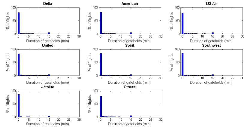
Figure 20: Histogram of duration of gate holds in minutes for the main seven carriers at LaGuardia. Data from July 1, 2013 to August 30, 2013 ... 66

Figure 21: New simulation process to include max hold conditions ... 67

Figure 22: Average taxi-out time by time of the day for the baseline and metering case. The metering strategy leads to a significant reduction in taxi-out time. Data from July 1, 2013 to August 30, 2013... 71

Figure 23: Average taxi-out time by terminal and by time of the day for the baseline and metering case. The metering strategy leads to a significant reduction in taxi-out time. Data from July 1, 2013 to August 30, 2013 ... 72

Figure 24: Average taxi-out time by runway configuration and by time of the day for the baseline and metering case. The metering strategy leads to a significant reduction in taxi-out time. Data from July 1, 2013 to August 30, 2013 ... 73

(11)

11

Figure 25: Use of runway configurations during July 2013 and August 2013.Runway

configurations 22|31 and 4|31 have approximately a joint 30% share... 75

Figure 26: Use of runway configurations during the metering periods on July 2013 and August

2013. Runway configurations 22|31 and 4|31 have approximately a joint 30% share. ... 75

Figure 27:Baseline (Strategy A) gate conflicts by time of day in blue and additional gate conflicts

by time of day when implementing Metering (Strategy B.Unr.). Data from July 1, 2013 to August

30, 2013... 78

Figure 28: Mean gate conflicts by time of day in three situations: mean of all days, week days and

weekends. Data from July 1, 2013 to August 30, 2013 ... 81

Figure 29: Mean gate conflicts by time of day in three situations: mean of days with RAPT larger

than 0 (“bad weather”), mean of days with RAPT equal to 0 (“good weather”). Data from July 1, 2013 to August 30, 2013 ... 82

Figure 30: Surface traffic, taxi-out times and gate-holding times for three MHP, compared with

the baseline cases. Data from July 9, 2013 ... 88

Figure 31: Policy B.15. histogram of duration of gate holds in minutes. Data from July 1, 2013 to

August 30, 2013 ... 94

Figure 32: Policy B.10. histogram of duration of gate holds in minutes. Data from July 1, 2013 to

August 30, 2013 ... 96

Figure 33: Variation of the percentage in taxi-out reduction with different gate-holding limits 100

Figure 34: Order differences between the take-off order and the EOBT order (ready for push order)

for the different gate-holding limit policies. Negative values correspond to flights that have been

moved backward in the departure line and positive values correspond to flights that have moved

(12)

12

is ready to push until the actual take-off time; which includes those coming from gate conflicts.

... 102

Figure 35: Order differences between the take-off order and the TOBT order (pushback order) for

the different gate-holding limit policies. Negative values correspond to flights that have been

moved backward in the departure line and positive values correspond to flights that have moved

forward in the departure line. This plot considers all the swaps after from the moment the aircraft

pushes until the actual take-off time, and thus it does not consider the swaps coming from gate

conflicts. ... 103

Figure 36: Order differences between the take-off order and the EOBT order for the different

airlines and for the two extreme gate-holding policies. Negative values correspond to flights that

have been moved backward in the departure line and positive values correspond to flights that have

moved forward in the departure line. ... 107

Figure 37: Prediction error with the estimated regression trees with a model time period of 15

minutes. ... 110

minutes. ... 111

(13)

13

LIST OF TABLES

Table 1: List of airlines operating out of each terminals at LaGuardia ... 26

Table 2: RAPT conversion table from numbers to colors ... 34

Table 3: Unimpeded taxi-out times (in minutes) for each terminal – runway configuration pair 41

Table 4: Standard deviation of the prediction error for regression trees with 15-, 30-, and 60-

minute time intervals... 44

Table 5: N-control values (# of aircraft) for each terminal – visual conditions pair ... 50

Table 6: Steps to simulate the departure procedure including gate conflict analysis and the

correction to include those conflicts in the model ... 62

Table 7: Additional row in Table 6 in order to include the maximum holding time condition. ... 67

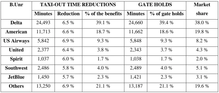
Table 8: Taxi-out time reductions (absolute and relative) and gate-holding time (absolute and

relative) for policy B.Unr. Data from July 1, 2013 to August 30, 2013 ... 93

relative) for policy B.15. Data from July 1, 2013 to August 30, 2013 ... 93

relative) for policy B.10. Data from July 1, 2013 to August 30, 2013 ... 95

Table 11: Table summarizing Table 8, Table 9, and Table 10. Data from July 1, 2013 to August

(14)

(15)

15

1. INTRODUCTION

Congestion is one of the major challenges currently faced by the U.S. National Airspace System

(NAS) and is expected to continue to experience in the foreseeable future. Although only a limited

number of airports experience mismatches between supply and demand, (De Neufville et al. 2013)

and are therefore congested, these airports have a large impact on the performance of the rest of

the network. Delays from these airports propagate to large parts of the system (Pyrgiotis 2012) due

to the network and complexity effects. The Joint Economic Committee of the U.S. Senate (Joint

Economic Committee 2008) estimated that in 2007, delays cost $40.7 billion to the U.S. economy.

The study considered airline operations, passenger cost and other economic activities, and

estimated that 20% of the delay costs correspond to the taxi-out phase. These costs include both

private and public components; taxi-out delays lead to additional engines-on time, which in turn

increases fuel burn for airlines, and emissions (particulate matter, carbon dioxide, hydrocarbons,

oxides of nitrogen, oxides of sulfur, among others) – a public cost for the society.

The goal of this thesis is to propose different policies to mitigate the effects of congestion, using

New York’s LaGuardia Airport as a case study.

1.1. SCOPE

Congestion occurs when the demand for a resource exceeds available capacity. There are broad

approaches to managing the problem of congestion at airports: infrastructure expansion, demand

management and airport surface management.

First, infrastructure expansions aim at solving the problem by increasing the physical infrastructure

(16)

16

capacity. However, there are several concerns with such an approach: first, infrastructure generally

requires large amounts of investments; second, there may not be space to expand the airport

(usually airports are constrained by the neighboring cities); finally, investing in infrastructure to

meet demand may turn into an unsustainable pattern from an environmental perspective.

Demand management, as described in (De Neufville et al. 2013), “refers to set of regulations or

other interventions aimed at constraining the demand for access to a busy airfield and/or at

modifying the temporal characteristics of such demand”. Demand management tries to limit access

to an airport through three main measures: overall demand reduction, demand limitations at

particular times, and demand shifts from high-demand to low-demand periods. Examples of

demand management approaches include schedule coordination (administrative strategy) and

congestion pricing (economic strategy), among others. In contrast to infrastructure expansion,

demand management aims at reducing demand to capacity levels through access control, instead

of increasing capacity to meet demand. Such an approach either denies access or charges a fee for

resources (arrival and departure rights).

Third, airport surface management manages the flow of aircraft at the airport during congested

periods in order to mitigate the impacts of congestion. It requires a detailed understanding of the

queuing processes taking place from the moment aircraft touch down until they take-off. The key

difference between surface management and the two previous strategies is that with this approach,

there is no change in the physical layout of the airport (capacity is the same) or the flight demand.

Thus the performance improvement arises from the way the traffic flows are managed. This

approach is the least capital intensive, and the least disruptive of the current everyday airline

(17)

17

Airport surface management deals with the following processes, which occur after the aircraft has

touched-down at the runway:

Figure 1: Airport surface processes

This research focuses on the departure part of the process, which corresponds to the last block of

processes in Figure 1.

1.2. DEPARTURE METERING-BASED POLICIES: DISCUSSION AND LITERATURE REVIEW

Departure metering is an airport surface management strategy that consists of holding aircraft at

the gate to avoid congestion at the runway in periods where the airport experiences saturation. In

this regard, Simaiakis (2013) reviews all the most relevant departure management algorithms and

classifies them as either trajectory-based models or flow-based (or Eulerian models). While the Arrival

• The aircraft taxies-in from the runway to ramp area and the gate.

Gate service

• Ground handlers ensure passenger service (de-boarding and boarding), baggage (unload and load), fueling, cleaning, and other services required to get the aircraft ready for pushback.

• The flight gets clearance from ATC (Air Traffic Control)

Departure

• The aircraft is ready for pushback • The aircraft pushes back

• The aircraft taxies-out

• The aircraft joins the departure queue • The aircraft takes-off

(18)

18

former optimizes the individual trajectory of each aircraft, the latter optimizes aircraft counts at

different control points; the actuation point in the context of this thesis is the gate, before the

pushback procedure. Using flow-based models involves creating virtual queuing approaches, as

initially suggested by Feron et al. (1997), and developed by Burgain, Feron, and Clarke (2008).

Indeed, the main rationale behind the proposed virtual queues is to ensure the fairness of aircraft

queuing without physically queuing at the runway. The virtual queue of concern here occurs at the

gate, with aircraft being held before their pushback procedure. A well studied Eulerian approach

is the N-control strategy (Pujet, Delcaire, and Feron 2003; Carr et al. 2002; Simaiakis 2009;

Simaiakis 2013). In addition to these references, the implementation of the N-control surface

management strategy at Boston Logan airport by Sandberg et al. (2014) sets a precedent in the

implementation of the proposed strategy.

The main benefits of the N-control metering strategy are the reduction of engines-on time, which

in turn leads to a reduction of fuel burn and greenhouse gas emissions. The trade-offs and impact

of surface operations to the environment has been analyzed by Simaiakis and Balakrishnan (2009);

Simaiakis and Balakrishnan (2010); Ravizza et al. (2013);and Khadilkar (2011), among others.

Building upon the N-control strategy framework developed above, this thesis presents three main

contributions:

 The thesis builds a model to implement an N-control surface strategy at LaGuardia Airport, learning from the lessons at Boston Logan Airport. Each airport presents fairly different

challenges and constraints that make the implementation of a surface control strategy an

ambitious task.

 The thesis proposes maximum gate-holding policies as well as a tool to evaluate these policies during the implementation design process. Metering strategies lead to significant

(19)

19

reductions in taxi-out times; however, pure metering may lead to operational challenges

for some stakeholders, especially if the gate-hold durations are high. This thesis develops

and evaluates a new portfolio of policies to bring flexibility during the implementation of

metering.

 The thesis updates previous studies of metering using RAPT (Runway Availability Prediction Tool) as a weather variable in addition to the visibility conditions (IMC/VMC).

RAPT is used as an independent variable in order to predict runway capacity. The statistical

analysis confirms the relevance of such an indicator as a runway capacity predicting

variable.

1.3. LAGUARDIA AIRPORT

This thesis focuses on analyzing the implementation of an airport surface control management

strategy at LaGuardia, one of the most congested airport in the U.S. In order to understand the

challenges and opportunities associated with airport surface congestion management, this section

presents fixed characteristics of the airport (those that are not likely to change in the short nor in

the medium term, such as airport layout, airport terminals, and some stakeholders) as well as

“dynamic” characteristics (those that may change in the medium term future, such as airline schedules).

1.3.1. AIRPORT CONGESTION

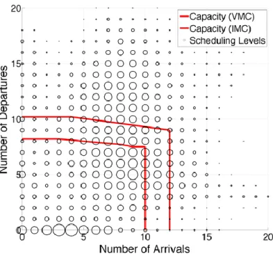
Figure 2 displays the results of a typical capacity analysis based on the concept of Operational

Throughput Envelope (OTE). An OTE is a curve in the 2-D space defined by the average number

(20)

20

represents the trade-offs between the arrival throughput and the departure throughput at the airport.

Put another way, “the envelopes indicate the capacity that can be achieved for all possible mixes of arrivals and departures” (De Neufville et al. 2013). For the case of LaGuardia, the interrelations of arrivals and departures are particularly relevant given the fact that the two runways intersect

and therefore, the capacity of the departing runway is affected by the performance in the arrival

runway. OTEs are a function of the runway configuration in use (i.e. set of runways used for

arrivals and departures) and the meteorological conditions. In Figure 2, the two OTEs correspond

to VMC1 (Visual Meteorological Conditions) and IMC2 (Instrument Meteorological Conditions), which, can generally be thought of as “good weather” and “bad weather” conditions, respectively. IMC always generates smaller average throughput than in VMC.

An OTE is generated as follows: First, from a rather large set of historic operational data from

departures in a particular period of time (in this case, 15-min periods), mathematical models are

used to build envelopes based on runway configuration and visibility conditions (Simaiakis 2013).

Second, using scheduling data, for each time period, the number of scheduled arrivals and number

of scheduled departures is computed and plotted. This observation may fall outside, inside, or on

the edge of the OTE. Figure 2 shows that, at LGA, significant imbalances between demand and

capacity may occur, as the scheduling leves fall frequently outside the area defined by the OTEs.

1_{VMC or Visual Meteorological Conditions: Aviation flight category in which visual flight rules (VFR)}

flight is permitted- that is, conditions in which pilots have sufficient visibility to fly the aircraft maintaining visual separation from terrain and other aircraft. They are the opposite of Instrumental Meteorological Conditions.

2_{IMC or Instrumental Meteorological Conditions: Aviation flight category that describes weather}

conditions that require pilots to fly primarily by references to instruments, and therefore under Instrument Flight Rules, rather than by outside visual references under Visual Flight Rules.

(21)

21

Note that these imbalances are, of course, more significant in IMC (“bad weather”). These

observations justify some intervention aimed at managing surface congestion.

Figure 2: OTEs envelopes at LGA for VMC and IMC, and scheduled number of flights. Source: (Simaiakis 2013; Jacquillat and Odoni 2015)

1.3.2. STAKEHOLDERS

In the context of this thesis there are four main groups of stakeholders:

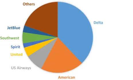
- Private carriers. This group includes all the airlines operating at the airport; the key among

which are Delta, American, US Airways, United, Spirit, Southwest, and JetBlue. Figure 3

depicts the relative number of operations of each airline for the July-August period in 2013.

During this Summer period, Delta Airlines, (including all of its regional and shuttle carriers

that offer services out of LGA) had nearly a 40% of the departures out of the airport; this

(22)

22

around 50%. The second largest carrier is American Airlines, with approximately a 20%

departure share, followed by US Airways, which holds approximately a 10%. The fourth

and fifth carriers are United and Southwest with a 5% market share each. In addition to

smaller participants such as Spirit or JetBlue, LaGuardia has a 20% of departures operated

by other airlines, which include general aviation and charter flights.

Figure 3: Departure share by carrier at LaGuardia Airport during the July-August 2013 period

- Airport-related institutions. There are two organizations with an essential role at LaGuardia

Airport:

o The Port Authority of New York and New Jersey (PANYNJ) is a Joint organization between the States of New York and New Jersey whose main mandate is to oversee

bridges, tunnels, airports and seaports around the New York City area. In the

context of this thesis, the PANYNJ is relevant because it oversees LaGuardia

Airport, JFK Airport and Newark Airport. Therefore, the PANYNJ has a large stake

in any change in airport operations (De Neufville et al. 2013). Delta American US Airways United Spirit Southwest JetBlue Others

(23)

23

o The Federal Aviation Administration is responsible of the Air Traffic Management in the United States, and thus, they decide on which air traffic management policies

to implement at all the airports in the country. In this thesis we propose new policies

to manage airport surface traffic which needs to be implemented by the FAA

controllers at the tower, and thus needs to be approved by the FAA.

- Passengers are important stakeholders in this thesis because they pay the costs of delays,

particularly with the lost opportunities.

- Society and the environment are relevant in this problem because the goal is to minimize

gas emissions and improve air quality. The former is salient given the significant

contribution of air transportation to greenhouse gas emissions, and the latter aims at making

to improve the life of people living in the neighborhoods surrounding the airport.

This thesis considers the main trade-offs among the interests of these stakeholders.

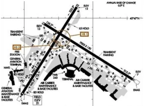
1.3.3. LAYOUT

This section introduces the physical layout of the airport, principally the runways, the terminals

and the taxiway system. Figure 4 clarifies of the overall layout of the airport. LaGuardia airport

has two crossing runways: one runway is oriented in the direction 4/223_{(S-SW/ N-NE)}4_{and the}

other in the direction 13/31 5(NW/SE).These two runways intersect and thus, as opposed to what

occurs with separated parallel runways, the departing traffic is greatly influenced by the arriving

traffic. Put another way, the intersection of runway diminishes the capacity compared with the

3_{Runways are referred to base on their orientation as indicated in (De Neufville et al. 2013)} 4_{South-South West/ North-North East}

(24)

24

situation when these runways can operate independently (De Neufville et al. 2013). However, there

are two advantages of having crossing runways: First, they can handle more capacity than a single

runway, and thus, in heavily urbanized areas like New York City, they allow more traffic despite

the land availability restrictions. Second, they allow arrivals and departures to operate in a variety

of weather conditions, particularly different wind directions.

Figure 4: LaGuardia Airport layout, including runways, taxiways and terminals. Source: Federal Aviation Administration, www.faa.gov

The combination of these two runways offers the airport of a portfolio of runway configurations

to process the arriving and departing flows. The usual terminology for runway configurations is

X/Y, where X is the arrival runway and Y the departing runway. In this regard, the most common

runways for the first months of 2013 are displayed in Figure 5. Five configurations (31|4, 22|31,

31|31, 22|13, and 4|13) are the most common in this eight-month period; the rest are not as used

(25)

25

to weather issues and noise protected areas in specific periods time. The importance of the five

mentioned runways is strengthened in Figure 6, which contains the runway configurations used

during the July-August 2013 period, which is the focus time period for this research.

Figure 5: Use of runway configurations during the eight months from January 2013 to August 2013

(26)

26

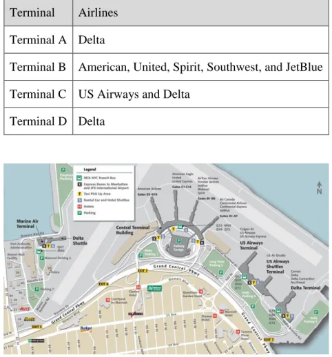
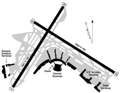
As for terminals, the airport has four terminals: A, B, C and D. In Figure 7 Terminal A is denoted

as the Marine Air Terminal, Terminal B as Central Terminal Building, Terminal C as the US

Airways Terminal, and Terminal D as the Delta Terminal. Despite the name of the terminals, they

do not quite represent the current operations at the airport due to some gate transfers between US

Airways and Delta. The main airlines under study operate from the following terminals:

Table 1: List of airlines operating out of each terminals at LaGuardia

Terminal Airlines

Terminal A Delta

Terminal B American, United, Spirit, Southwest, and JetBlue

Terminal C US Airways and Delta

Terminal D Delta

Figure 7: Map of the four terminals at LaGuardia Airport. Source: Port Authority of New York and New Jersey, www.panynj.gov

(27)

27

The next airport layout factor to comment on is the taxiway system, which allow aircraft to travel

to and from the terminal and the runway. Figure 4 depicts the network of taxiways at LaGuardia

Airport.

The airport is constrained by the limited surface available, and that translates to a limited number

of taxiways. Such a taxiway system has three important aspects worth noting:

- There is only one taxiway feeding runway 4 | 22 in the southernmost part of the airport,

taxiway B. This is particularly salient for departures from runway 4; indeed, in cases of

high demand, the departure queue of more than 30 aircraft can use the taxiway up to just

before the runway crossing. As for the taxiway AA, parallel to the runway to the left, is

mainly used by aircraft operating from Terminal A, in the westernmost area of the airport.

- There are two taxiways parallel to runway 13 | 31, taxiways A and B. These two runways

bring flexibility to airport operations, particularly in two circumstances:

o During periods when the 31 is used as departure runway, these two taxiways are the departure feeders; however, one taxiway is assigned to manage arrivals and the

other to departures. By doing so, traffic is not mixed and there is more

predictability. Such a strategy should facilitate surface operations without creating

additional challenges, and that is why, in case one taxiway is blocked, aircraft may

use the other to overcome such blockage.

o During periods when runways 4, 22, or 13 serve as departure runways, one taxiway is used for eastbound movements and the other for westbound movements. Such a

strategy avoids situations with two aircraft facing each other.

- The taxiway density in the eastern area of the intersection is higher than in other areas of

(28)

28

demand. Taxiing out to runway 13 may be longer and less predictable from aircraft

travelling from terminals B, C, and D, because they need to first cross the runway and then

wait for their “take-off slot”. Such a waiting time requires aircraft to be able to wait in that area without interfering with the arrival traffic. To this end, taxiways, AA, BB, and CC

classify aircraft before take-off.

1.4. OUTLINE

This thesis describes the problem of congestion at a constrained airport, focuses on airport surface

departure management, proposes a control strategy and, finally, has presentes the characteristics,

opportunities and challenges of implementing such a strategy at LaGuardia Airport.

The remainder of this thesis delves deeper into the model and evaluates its performance. Chapter

2 describes the different approaches to airport surface departure control, and derives several

control policies based on the strategies described; this description includes mathematical

formulation, estimation of parameters, and compilation of data; Chapter 3 presents the

performance results of the strategies and policies presented in Chapter 2; finally, Chapter 6

concludes this thesis, summarizing the findings, recommending policies and indicating next

(29)

29

2. MODEL

This chapter presents the details of the mathematical model built to compare two airport surface

control strategies: Pushback-at-discretion (Strategy A), and Metering (Strategy B); the former

represents the status quo, and the latter is the proposed strategy that is being evaluated throughout

the thesis. Section 2.1 introduces a general overview of the two strategies. Evaluation and

assessment of these strategies is done using three datasets: ASPM (Federal Aviation

Administration), flightstats (www.flighstats.com), and RAPT (MIT Lincoln Labs). Based on the

model requirements, the chapter then introduces the parameters, mathematical tools, and variables

that need to be input to the model. One issue that arises when building the model is gate conflicts,

which are a consequence of the increase in the time aircraft spend at the gate. Thus, the next section

lays out ways to include into the model. Drawing upon all this information, the chapter presents

the mathematical formulation associated with each strategy.

2.1.AIRPORT SURFACE CONTROL STRATEGIES FOR DEPARTING TRAFFIC

The strategies below represent two different ways of managing the departing flow aircraft from

the moment each aircraft is ready for pushback (in aviation jargon, off-block time6), until the

aircraft takes off (in aviation jargon, Wheels off-time7 or Take-off time). As indicated, this section

6_{Off-block time: Time at which the aircraft is ready to start the pushback process. The term block refers}

to the physical objects that are put in front and behind the wheels to prevent de aircraft from moving at all.

7 Wheels-off time: the moment the aircraft is rolling on the runway and the wheels lose physical contact with the runway due to lift. Wheels-off refers to the moment when the wheels are off the runway.

(30)

30

only provides a brief general overview/introduction to these strategies so that the reader can have

a general understanding of all the components required for the model.

Before plunging into the description and comparison of the two strategies, it is helpful to introduce

a time framework to analyze the processes in a systematic way. Indeed, defining key milestones

in the departure process provides a clear pattern for comparison and simulation (as presented later

in the thesis). The time framework has four key milestones:

 EOBT8_{: Earliest Off-Block Time. Earliest time an aircraft is ready to start the pushback}

procedure

 TOBT: Target Off-Block Time. Time that an aircraft is authorized to start the pushback

 DQET: Departure Queue Entry Time. Time when the aircraft joins the physical queue of aircrafts waiting to take-off that starts at the runway heading and growths through the

taxiway system. An aircraft joins this queue after taxiing from the gate the queue.

 ATOT: Actual Take-Off Time. Wheels-off time for each aircraft

Having this framework in mind, it is possible to introduce and compare the two strategies. In

particular, this framework is interesting to look at these other parameters.

 GHT: Gate-holding Time or Gate Hold. Time an aircraft is being held at the gate, “prevented” from starting the pushback procedure. Using the framework introduced above,

GHT=TOBT-EOBT.

 EOT: Engines On Time. Total time departing aircraft spends with the engines on burning fuel and emitting gases while on the airport surface. The assumption in this thesis is that

8_{For clarity purpose, EOBT, TOBT, DQET, and ATOT in capital letters will refer to the general variable,}

whereas when referring to values of these variables for specific flights this thesis uses non capitalized letters: eobt(i), tobt(i), dqet(i), atot(i)

(31)

31

pilots switch on engines slightly before TOBT and keep them on after that. Hence, in the

context of airport departure surface operations, EOT= ATOT-TOBT.

 TOT: Taxi Out Time. Time a departing aircraft spends travelling through the taxiway system. This parameter coincides with the time the aircraft has its engines on, and hence

TOT=EOT.

This framework will allow us to analyze the performance of strategies A and B throughout this

thesis.

2.1.1. STRATEGY A:PUSHBACK-AT-DISCRETION

Pushback-at-discretion, from now referred to as Strategy A or the baseline case, represents the way

the majority of airports handle the departure processes. The main essence of such a strategy is that

aircraft pushback whenever they are ready; put another way: EOBT=TOBT. Given the uncertainty

in airport operations (Hall and Fernandes 2013) and the lack of schedule coordination in the U.S.

(De Neufville et al. 2013), it is common to see long departing queues at the runway. In other words,

with this strategy, when aircraft pushback, they do not know what the current queue length at the

runway is, and therefore, after pushing back, they taxi to the runway, join the queue, regardless of

the length, and eventually take off. Based on this, it is difficult to set up a straightforward

relationship between DQET and ATOT. As far as the EOT taxi concerns, it is worth noting that the

lack of information on the congestion situation downstream generates useless idling time with the

engines on.

In the baseline case aircraft push back at EOBT (EOBT=TOBT), then, the aircraft taxies out for an

uncertain amount of time until they join the queue at time DQET and then, after all the aircraft in

(32)

32

It is clear that information in this strategy propagates only downstream. Indeed, there is no

information moving upstream. As a consequence, airlines have an incentive to adopt the following

attitude: the earlier I join the queue, the earlier I will take off.

2.1.2. STRATEGY B:METERING

Metering consists of holding aircraft at the gate long enough to avoid, as much as possible, the

inefficient idling time at the departing queue, without interfering much with the take-off time. In

order to do that, this strategy propagates the information upstream, instead of downstream. The

model carries out the following process: first, it evaluates the runway departure capacity; second,

it propagates this departure capacity through the taxiway system into the terminal, and finally,

recommends a pushback rate. Put another way, the model converts runway capacity into “pushback capacity”, and aims at limiting the number of aircraft on the surface causing congestion, allowing the pushback procedure only to the number of aircraft that will sustain departure capacity without

creating unnecessary congestion. This upstream information process requires two tools to predict

departure runway capacity, and the propagation of this runway capacity through the taxiway

system. These tools are regression trees and saturation plots and will be addressed in section 2.3.

At this point it is possible to broadly put this proposed strategy into the time framework introduced

above. The first difference between the two strategies is that EOBT is not necessarily equal to

TOBT due to the definition of gate hold. Indeed, a gate hold is the situation in which an aircraft is

“prevented” from starting its pushback procedure despite being ready to do so. It is important to note that gate holds do not occur all the time, and therefore, there may be instances when EOBT

(33)

33

regard, section 2.6 explains the details about the conditions in which gate holds occur and the way

the model determines TOBT.

As for DQET and ATOT, the difference from Strategy A is that in circumstances when aircrafts

are held, the difference between ATOT and DQET is smaller, and so is the EOT, which is the main

reason why reductions in emissions and fuel burn exist.

2.2. DATASETS

This research requires two main types of data, weather data and airport scheduling data. As for the

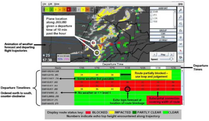
meteorological data, the model uses a weather predictability tool called RAPT (DeLaura et al.

2008), which stands for Route Availability Prediction Tool, and was developed by Lincoln

Laboratory with the main goal of helping air traffic controllers at airports severely affected by

convective weather9_{, as is the case of LaGuardia Airport. This tool is effective at analyzing how}

available a particular air route is on a scale from 0 to 3, where 0 is good weather and 3 corresponds

to a route being totally blocked by convective weather and thus, inoperative. In the tower, the

numbers are converted into colors and the conversion is the following:

9_{Convective weather: In meteorology, the term is used specifically to describe vertical transport of heat}

and moisture in the atmosphere, especially by updrafts and downdrafts in an unstable atmosphere. The terms "convection" and "thunderstorms" often are used interchangeably, although thunderstorms are only one form of convection. Cbs, towering cumulus clouds, and ACCAS clouds all are visible forms of convection. However, convection is not always made visible by clouds. Convection which occurs without cloud formation is called dry convection, while the visible convection processes referred to above are forms of moist convection. Source: www.forecast.weather.gov

(34)

34

Table 2: RAPT conversion table from numbers to colors

Number Color Weather implications

0 Green Clear

1 Dark Green Low Impact

2 Yellow Caution

3 Red Blocked

Taking this color code into account, it is possible to understand the RAPT display that air traffic

controllers have in the tower, on which they base their decisions. Figure 8 shows such a display,

where it is possible to see the different colors available for different routes; such information helps

controllers decide upon which route to guide the flow of aircraft through, both arrivals and

departures based on the weather situation.

(35)

35

For the case of this research, the RAPT indicator used is an average all the routes operated to/from

the airport. This tool is rather intuitive given its straightforwardness to understand and interpret;

however, it is challenging to associate the non-integer numbers (such as 1.67) with the real weather

meaning. For the purpose of this research, RAPT is a given variable that is used as a proxy for

weather, and as proven throughout the thesis, RAPT is an effective variable for considering

meteorological conditions in the context of airport performance.

Regarding the airport scheduling data, this research uses two complementary datasets. On the one

hand, the model is fed and most of the parameters are calibrated using the ASPM dataset, which

stands for Aviation System Performance Metrics and is developed by the FAA10. The most

interesting variables from the ASPM dataset are the mentioned below, but the most relevant aspect

here is that the information provided is granular, as the data is presented at a flight level, which

means that all the parameters are shown flight by flight:

 Airline (Arrivals & Departures)

 Flight number (Arrivals & Departures)

 Runway configuration (Arrivals & Departures)

 Visibility conditions at LGA (Arrivals & Departures)

 Arrival Actual Wheels-on time: Time at which the aircraft put its wheels on the runway.

 Departure Actual call time: Time at which the flight is ready and calls for pushback. In the framework presented above, this time is equivalent to the Earliest Off-Block Time, EOBT.

 Departure Wheels-Off time: Time in the departure roll when the flight lifts off the ground. In the framework presented, this is equivalent to the Actual Take-Off Time, ATOT.

(36)

36

It is worth noting that there are two key important data missing: terminal building and gate at

which each flight is serviced. This lack of data is what makes the second dataset detrimental for

the model; indeed, the model needs flight-specific information on terminal and gate from where

the flight is being operated. On the one hand, the terminal information is required to incorporate

into the model the pros and cons of operating at each specific terminal, particularly the most salient

fact being the difference in taxi-out time that may affect the order dynamics on the surface. On the

other hand, the gate information is necessary, when evaluating and avoiding gate conflicts caused

by the implementation of the metering strategy. Based on these needs, the second dataset is

obtained from the flightstats website11, which offers flight level details based on generic FAA

datasets, but the website buys additional information to airlines in order to provide a better service.

In particular, the website adds terminal and gate information, which is of great relevance for this

research.

Finally, it is important to clarify the time span of each dataset. Given the way ASPM data is

compiled, it is possible to obtain fairly long records of data, and that is the reason why this research

uses data from June 2012 until August 2013. However, flightstats data is more cumbersome to

obtain as need to be pulled out in 2-hour periods and thus, only strictly necessary data is gathered.

This difficulty has some consequences in the parameter estimation as explained in the next section.

2.3. PARAMETERS, MATHEMATICAL TOOLS, AND VARIABLES

This section introduces several parameters, tools and variables that the model requires, and are

important to describe before plunging into the model analysis. In particular, this section introduces

the concept of unimpeded taxi-out time, decides the length of the time steps used for the simulation,

(37)

37

and finally presents the two prediction tools required to implement metering, characterized by the

upstream flow of information.

2.3.1. UNIMPEDED TAXI-OUT TIME

The unimpeded taxi-out time is the taxi-out time that allows the model to simulate a congestion

free situation; however, this is a rather broad and unspecific definition. To this end, Simaiakis

(2013) carries out a review of different ways unimpeded taxi-out time can be defined. The general

definition is the nominal, free flow taxi out time, which is related to the absence of obstacles in the

taxi-out process. The FAA definition is the following: “taxi-out time under optimal operating

conditions, when neither congestion, weather nor other factors delay the aircraft during its

movement from the gate to take-off” (Office of Aviation Policy and Plans, Federal Aviation

Administration. 2002). From this definition and based on Simaiakis (2009), the following

statements can be made:

 The unimpeded taxi-out time is not the minimum taxi-out time; it actually is the average taxi-out time when there is no departure queue.

 Talking about average values is reasonable given that taxi-out times are random variables. Several factors that come into play in this random process are: use of different taxiway

routes, use of different speeds, differences in the duration of the pushback process,

differences in the process of engine start, or variations in the controller-pilot

communications.

 The unimpeded taxi-out time is an average value, which implies than is the result of a calculation, not an observation.

(38)

38

In addition to these observations, it is worth noting that the unimpeded taxi-out time has a weak

correlation with the number of aircraft taxiing-out on the surface at the pushback time of each

flight (Idris et al. 2001). This is because such an indicator does not consider factors such as aircraft

pushing back later but still affecting the taxi-out process of the flight. In order to correct this

mismatch, Idris et al. (2001) suggest using the concept of take-off queue for a particular flight,

defined as the number of aircraft taking off between the pushback and take-off time of that flight;

after describing the concept, they also suggest using such a concept to predict taxi-out times.

Based on all these considerations, Simaiakis (2013) sets up the following to estimate the

unimpeded taxi-out time. First, he defines Effective traffic “for each aircraft l, Neff(l), as the sum if the aircraft taxiing out, N(l), at the time of the flight’s pushback t, and the number of aircraft that

push back while it is travelling to the departure runway”. From a data availability standpoint, Neff(t) requires the model to be fed with the ASDE-X12_{dataset, a more detailed and granular dataset}

compared to the ASPM the dataset. Clewlow (2010) suggested using another indicator, the

adjusted traffic, which is equivalent to the effective traffic at being well correlated with the

taxi-out time, but it can be obtained from ASPM datasets, which makes the simulations simpler but

12_{ASDE-X enables air traffic controllers to detect potential runway conflicts by providing detailed} coverage of movement on runways and taxiways. ASDE-X collects data from a variety of sources to track vehicles and aircraft on the airport movement area and obtain identification information from aircraft transponders. The ASDE-X data comes from surface movement radar located on the air traffic control tower or remote tower, multilateration sensors, ADS-B (Automatic Dependent Surveillance-Broadcast) sensors, the terminal automation system, and aircraft transponders. By fusing the data from these sources, ASDE-X is able to determine the position and identification of aircraft and transponder-equipped vehicles on the airport movement area, as well as aircraft flying within five miles of the airport. Source:

(39)

39

equally effective. Adjusted traffic is defined for “each aircraft l, as the aircraft taxiing out, N(l), at

the time of its pushback t, and the number of aircraft that push back while aircraft l is taxiing out”.

The interesting aspect of both the effective and adjusted traffic is the consideration of the traffic

ahead while pushing back as well as the traffic that joined while the aircraft is taxiing-out in order

to consider all the aircraft that can interfere with this flight’s trajectory.

Then the model computes the empirical unimpeded taxi-out time as the time corresponding to the

adjusted (as a proxy for the effective) traffic for which the taxi-out time does not increase, with increasing effective traffic. To calculate the empiric taxi-out time, it is necessary to use historic

data to compute, for each flight, the effective traffic and the observed taxi-out time. Then, for each

subcategory of flights, create a scatter plot as seen in Figure 9 with the effective traffic on the

x-axis and the taxi-out time in y-x-axis. For each subcategory we understand all the combinations of

factors based on which the results are displayed; in this case results are shown by terminal and

runway configuration. For example, the effective traffic and the observed taxi-out time of all flights

leaving from terminal B when there is runway configuration 22|31 are depicted in a scatter plot as

seen in Figure 9.

These scatter plots allow the model to run a convex optimization regression to fit a non-decreasing,

and convex function to the observed data. Such a curve would predict the taxi-out time as a

function of the adjusted traffic. As described in (Simaiakis 2013),

Given m pairs of measurements Nadj(l) and τ(l), denoted (u1,y1), …, (um,ym), we seek a convex, non-decreasing function fmean: ℝ →ℝ that estimates the mean τ=f(Nadj(l)). This infinite-dimensional problem is significantly simplified by the fact that Nadj is defined only

in the domain of natural numbers (ℕ0). f can be restricted to within the domain of ℕ0 as

(40)

40

f is simply a piecewise linear function of N, and the monotonicity and convexity constrains

are imposed at the points 0,1, ..., max(Nadj) by comparing the values and the slopes of a subsequent pieces. f is given by the solution to the following convex optimization problem:

𝑚𝑖𝑛 ∑(𝑦̂_𝑖 − 𝑦_𝑖)2 𝑚 𝑖=1 subject to: 𝑦̂_𝑖 = 𝑓(𝑢_𝑖), 𝑖 = 1, … , 𝑚 𝑓(𝑖 + 1) ≥ 𝑓(𝑖), 𝑖 = 0, … , (𝑛 − 1) 𝑓(𝑖 + 1) − 𝑓(𝑖) ≤ 𝑓(𝑖) − 𝑓(𝑖 − 1), 𝑖 = 1, … , (𝑛 − 1) Eq. 1

Figure 9: Scatter plot with taxi-out time as a function of the adjusted traffic for flights from terminal B when the runway configuration was 22|13. Data from July 1, 2013 to August 30, 2013

Solving this mathematical problem we obtain the non-decreasing and convex functions, as

(41)

41

for each runway configuration and terminal. Table 3 displays the empirical unimpeded taxi-out

times, which have been obtained by identifying in each non-decreasing, and convex function, the

minimum value of the function.

Figure 10: Mean, standard error, and fit function from the scatter plot in Figure 9 for flights from Terminal B when the airport operates with runway configuration 22|13. Data from July 1, 2013 to August 30, 2013

Table 3: Unimpeded taxi-out times (in minutes) for each terminal – runway configuration pair

31|4 22|31 31|31 4|31 13|13 22|13 4|13 13|4 22 31|31 4|4

T-A 13.92 12.96 12.74 13* 12* 13.6 13* 12* 9.9 12.95

T-B 13.22 10.72 11.39 11* 12* 13.07 14* 12* 14.36 12.41

(42)

42

For clarification purposes, the values with an * have been interpolated from configurations with

the same departing runway, given that the pool of observations for that configuration was too small

to obtain a reliable enough number.

Another important comment is the reason behind merging Terminal C and Terminal D together.

The ASPM dataset does not contain information on terminal or gates; therefore, we need to filter

the ASPM dataset by other parameters to indirectly obtain data at a terminal level. Indeed, we

identified those airlines and destinations (data available in the ASPM dataset, for each flight) that

are served in each terminal, and that provided the model with a de facto terminal based

classification. Unfortunately, it was not possible to find a clear classification pattern for Terminals

C and D because Delta operates from both terminals and in particular, it serves one same

destination from different terminals. This inability to classify flights from terminals C and D is the

reason for a combined calculation of unimpeded taxi-out times.

After these two clarifying comments, the results in Table 3 give a sense of the length of typical

free-flow taxi-out length; however, it is difficult to compare rows from that table because different

terminals have different challenges and different layouts, as can be grasped from the LaGuardia

layout in Figure 11. One example of such a challenge is the need for departing flights from

Terminal A to cross arrival runway 22 when the departing runway is 31, which is likely to add

additional time to the taxi-out time. Another challenge is the availability of handling resources.

Recalling that the pushback procedure is one of the key variables affecting the unimpeded taxi-out

time, the main carrier in terminal C and D, Delta, has a limited number of resources (tugs and

manpower) to serve departing flights. Having more flights to serve with shared resources may

affect the efficiency with which Delta carries out pushback. Nevertheless, this is just an example

(43)

43

an explanation it would be necessary to carry out a resource availability benchmark that would

allow us to compare each carrier’s performance.

Figure 11: LaGuardia Airport layout, including runways, taxiways and terminals. Source: www.faa.gov

2.3.2. TIME PERIOD LENGTH

At this point we need to decide the length of the simulation time period. This time period is the

time fraction in which the model breaks out all days in order to implement a discretized analysis.

That is, in order to implement the metering strategy, it is necessary to divide up the whole day into

smaller segments. However, choosing the time period length of the simulation is not a

straightforward decision. It is, indeed, a key decision and it has different types of implications of

which it is worth being aware. The time period length is a trade-off between computational cost,

prediction accuracy, usefulness during implementation, and synchronization with the structure of

the model and other parameters. These four aspects separately would lead to opposite time period

(44)

44

First, from a computational cost point of view, the shorter the time period, the more costly it

becomes. Indeed, shorter periods mean more periods and thus, the model needs to carry out a

similar routine more time. Therefore, from a computational cost standpoint, the longer the period,

the better.

Second, from the prediction accuracy perspective, the shorter the time period, the better. In order

to understand such a statement, it is necessary to understand how predictions are carried out. In a

nutshell, at the beginning of each period, the algorithm predicts a departure capacity and a

pushback rate derived from parameterized tools presented below. From an ongoing work we have

seen that the accuracy of these tools becomes less reliable as the length of the time period increases.

One particular example of such a trend is the worsening of success rates from the regression trees

(presented in section c below), which are being used to predict runway capacity. Table 4 shows

that the standard deviation of the error for regression trees increases as the time period length

increases, which makes the predictions less reliable.

Table 4: Standard deviation of the prediction error for regression trees with 15-, 30-, and 60- minute time intervals.

Time period length 15-minute 30-minute 60-minute

Standard deviation of the error 1.7 (dep/15-min) 3.6 (dep/30-min) 6.2 (dep/60-min)

Such a worsening trend can be extrapolated to the other tools used at the beginning of each time

period. Analyzing the data we can see that the main reason for this behavior is the uncertainty, and

particularly the noise. The larger the time period length, the more the noise and thus, the poorer

(45)

45

Third, the usefulness during implementation phase has not much to do with the mathematical

capability and strengths of the model; it concerns mainly the effectiveness when being

implemented in reality. In particular, as indicated in coming sections, the main goal of metering is

to suggest a pushback rates to controllers, who then communicate with airlines to give them a

prediction of the expected time to start the pushback procedure (TOBTs). One of the strengths of

such an approach is the ability to predict, at the beginning of each period, the TOBTs for the

duration of the period. This information is greatly appreciated by airlines given that gate-holdings

may represent a disruption to them. With such information, airlines can plan their handling

resources accordingly. However, the value of this information decays with short notice. That is,

information on TOBTs provided 15 minutes in advance is significantly more useful than that

information provided 5 minutes in advanced as the ability to plan around it is more salient in the

former case than in the latter. Based on such facts, the longer the time period, the more valuable

the information provided to airlines is.

Fourth, and last, the synchronization with the structure of the model and other model parameters

concerns how this time period lengths fits with the other model components. In particular, given

that the model updates predictions and allocations of TOBTs at the beginning of the time period,

it is important to match its time length with the dynamics of what happens in that time period. On

particularly important factor is the unimpeded taxi-out time, which, as has been shown already,

has values around 15 minutes. This makes a very good case to fix the time length to 15 minutes.

Indeed, having a time period length similar to the taxi-out time helps isolate the performance of

different flights occurring in different time periods. In particular, all the flights that started their

(46)

46

of flights that is relevant in those cases where there is a change in airport performance conditions

in these two periods.

This fourth point justifies the use of a 15-minute time period as opposed to a shorted or longer

duration. We believe that 15 minutes is ideal as it leads to a reasonable computational load, it

results in rather accurate results, and provides valuable information to airlines to allocate resources

based on potential disruptions caused by metering.

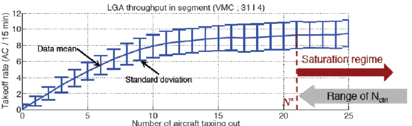
2.3.3. SATURATION PLOTS

The next step of the parameter estimation process is to develop one of the two predictive tools that

allow the propagation of runway capacity information to pushback information. The tool used for

such a task is the saturation plots and its main goal is to measure the capacity of the airport surface.

This representation, introduced by Shumsky (1995) and Pujet (1999), presents the surface traffic

N, on the y-axis, and then the departure throughput DT, on the y-axis, as a function of N, as depicted

in Figure 12.

(47)

47

Figure 12 shows that, initially, the departure throughput increases as the surface traffic increases;

however, this behavior only occurs up until a saturation point, when demand exceeds the critical

value, N*. From Figure 12, the N* value is 21 and the take-off throughput at saturation is

approximately 9 aircraft every 15 minutes. This N* can be seen as an intrinsic value of the airport,

given that it is operating under a particular runway configuration. Knowing this value, the operator

can decide to use it as a control threshold in order to avoid excessive aircraft on the surface. And

therein lies the difference between what the literature (Sandberg et al. 2014; Simaiakis et al. 2011)

refers to as N-Control and N*. N-control (Nctrl) is the value that the operator may decide to set as

a threshold, and N* is an airport configuration-specific characteristic that cannot be modified

unless the airport physical characteristics change. This difference leads to the ideal Nctrl discussion.

First, Nctrl always has to be larger than N*, otherwise the model would likely be starving the

runway, and thus not using the runway capacity efficiently. Second, there is some reluctance to

change from the current state which corresponds to Nctrl equal infinity, which is the same as no

control of the surface traffic. Such reluctance translates into a pressure to control significantly

above the N* value. That is finally a policy decision made by the operator. However, in the context

of this research, metering –primarily dependent on the value of Nctrl- is associated with Nctrl = N*.

Considering all the above, the model derives the throughput-surface traffic function, fitting a curve

to observed data from the ASPM dataset for the first 8 months of year 2013. Indeed, for each

15-minute period, we calculate the surface traffic demand N(t) - defined as the number of aircraft that

have pushed back from their gates, but have not yet taken off, and the departure throughput DT(t)

- defined as the number of aircraft that take off during the time period of analysis. Then the model

implements rather similar to the model used to obtain the unimpeded taxi-out time, except for the

(48)

non-48

decreasing and concave function that links departure throughput and departure demand

(independent variable), based on the observed pairings of [N(t), DT(t)]. As presented by Simaiakis

(2013):

The estimation of the data mean regression fit can be formulated as a least-squares problem.

Given m pairs of measurements N(t) and DT(t), denoted (u1,y1),…,(um,ym), we seek a non-decreasing, concave function fmean: R →R that estimates the mean DT= fmean(N) This

infinite dimensional problem is significantly simplified by the fact that N is defined only in the domain of natural number (N0). fmean can be restricted in the domain of N0 as well, and we need to estimate the values fmean (0), fmean (1), …, fmean (n), where n=max(Nadj). The function fmean is simply a piecewise linear function of N, and the monotonicity and

concavity constrains are imposed at the points 0,1, ..., max(Nadj) by comparing the values and the slopes of a subsequent pieces. fmean is given by the solution to the following convex

optimization problem: 𝑚𝑖𝑛 ∑(𝑦̂𝑖− 𝑦𝑖)2 𝑚 𝑖=1 subject to: 𝑦̂_𝑖 = 𝑓_{𝑚𝑒𝑎𝑛}(𝑢_𝑖), 𝑖 = 1, … , 𝑚 𝑓_{𝑚𝑒𝑎𝑛}(𝑖 + 1) ≥ 𝑓_{𝑚𝑒𝑎𝑛}(𝑖), 𝑖 = 0, … , (𝑛 − 1) 𝑓𝑚𝑒𝑎𝑛(𝑖 + 1) − 𝑓𝑚𝑒𝑎𝑛(𝑖) ≤ 𝑓𝑚𝑒𝑎𝑛(𝑖) − 𝑓𝑚𝑒𝑎𝑛(𝑖 − 1), 𝑖 = 1, … , (𝑛 − 1) Eq. 2

A similar process is proposed by Simaiakis (2013) to estimate the median throughput as a function