Bayesian Computation through Cortical Latent Dynamics

Bayesian Computation through Cortical Latent Dynamics

The MIT Faculty has made this article openly available.

Please share

how this access benefits you. Your story matters.

Citation

Sohn, Hansem et al. “Bayesian Computation through Cortical Latent

Dynamics.” Neuron, 103, 5 (September 2019): 934–947.e5 © 2019

The Author(s)

As Published

10.1016/J.NEURON.2019.06.012

Publisher

Elsevier BV

Version

Author's final manuscript

Citable link

https://hdl.handle.net/1721.1/130521

Terms of Use

Creative Commons Attribution-NonCommercial-NoDerivs License

Bayesian computation through cortical latent dynamics

Summary

Statistical regularities in the environment create prior beliefs that we rely on to optimize our behavior when sensory information is uncertain. Bayesian theory formalizes how prior beliefs can be leveraged and has had a major impact on models of perception, sensorimotor function, and cognition. However, it is not known how recurrent interactions among neurons mediate Bayesian integration. Using a time interval reproduction task in monkeys, we found that prior statistics warp neural representations in the frontal cortex allowing the mapping of sensory inputs to motor outputs to incorporate prior statistics in accordance with Bayesian inference. Analysis of recurrent neural network models performing the task revealed that this warping was enabled by a low-dimensional curved manifold, and allowed us to further probe the potential causal underpinnings of this computational strategy. These results uncover a simple and general principle whereby prior beliefs exert their influence on behavior by sculpting cortical latent dynamics.

Graphical Abstract

¶_{Corresponding author and lead contact Mehrdad Jazayeri, Ph.D., Robert A. Swanson Career Development Professor, Associate} Professor, Department of Brain and Cognitive Sciences, Investigator, McGovern Institute for Brain Research, Investigator, Center for Sensorimotor Neural Engineering, MIT 46-6041, 43 Vassar Street, Cambridge, MA 02139, USA, Phone: 617-715-5418, Fax: 617-253-5659, mjaz@mit.edu.

*Equal contribution Author contributions

H.S. and M.J. conceived the in-vivo experiments. H.S. collected the physiology data. D.N. and M.J. conceived the in-silico experiments with recurrent neural networks. D.N. trained, simulated and analyzed the networks. H.S. and N.M. analyzed the physiology data. M.J. supervised the project. All authors were involved in interpreting the results and writing the manuscript. +Department of Brain & Cognitive Sciences, McGovern Institute for Brain Research

Publisher's Disclaimer: This is a PDF file of an unedited manuscript that has been accepted for publication. As a service to our customers we are providing this early version of the manuscript. The manuscript will undergo copyediting, typesetting, and review of the resulting proof before it is published in its final citable form. Please note that during the production process errors may be discovered which could affect the content, and all legal disclaimers that apply to the journal pertain.

DATA AND CODE AVAILABILITY

The published article includes all datasets generated or analyzed during this study. The code supporting the current study is available from the corresponding author on request.

HHS Public Access

Author manuscript

Neuron

Published in final edited form as:

Neuron. 2019 September 04; 103(5): 934–947.e5. doi:10.1016/j.neuron.2019.06.012.

A

uthor Man

uscr

ipt

A

uthor Man

uscr

ipt

A

uthor Man

uscr

ipt

A

uthor Man

uscr

ipt

eTOC

Sohn, Narain, Meirhaeghe et al. found that prior beliefs warp neural representations in the frontal cortex. This warping provides a substrate for the optimal integration of prior beliefs with sensory evidence during sensorimotor behavior.

Introduction

Past experiences impress upon neural circuits information about statistical regularities in the environment, which helps us in all types of behavior, from reaching for one’s back pocket to making inferences about others’ mental states. There is, however, a fundamental gap in our understanding of how behavior exploits statistical regularities in relation to how the nervous system represents past experiences. The effect of statistical regularities on behavior is often described in terms of Bayesian theory, which offers a principled framework for

understanding the combined effect of prior beliefs and sensory evidence in perception (Knill and Richards, 1996), cognition (Thomas L. Griffiths et al., 2008), and sensorimotor function (Körding and Wolpert, 2004). On the other hand, the effects of experience on neural activity have been described in terms of cellular mechanisms that govern the response properties of neurons. For example, natural statistics are thought to shape response properties of early sensory neurons through adjustments of synaptic connections (Girshick et al. 2011;

Simoncelli and Olshausen 2001; Berkes et al. 2011; Fiser et al. 2010). Single-unit responses in many brain areas are though to encode recent sensory events (Akrami et al., 2018), motor responses (Darlington et al., 2018; Gold et al., 2008; Janssen and Shadlen, 2005), reward expectations (Platt and Glimcher, 1999; Seo et al., 2014; Sugrue et al., 2004), and temporal

A

uthor Man

uscr

ipt

A

uthor Man

uscr

ipt

A

uthor Man

uscr

ipt

A

uthor Man

uscr

ipt

contingencies (Narain et al. 2018). However, an understanding of how experience-dependent neural representations enable Bayesian computations is lacking.

Recent studies have focused on an analysis of the structure of in-vivo cortical activity in trained animals and in-silico activity in trained recurrent neural networks (RNNs) to gain a deeper understanding of how neural populations perform computations (Churchland et al., 2012; Chaisangmongkon et al., 2017; Mante et al., 2013; Remington et al., 2018a; Wang et al., 2018; Yang et al., 2019). Following this emerging multidisciplinary approach, we analyzed the structure of neural activity in the frontal cortex of monkeys and in-silico activity in RNNs in a Bayesian timing task. Results provided evidence that prior statistics establish curved manifolds of neural activity that warp the underlying representations of time and cause biases in accordance with Bayesian integration.

Results

Task and behavior

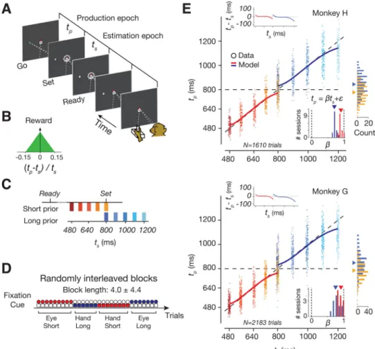
Two rhesus macaques performed a time-interval reproduction task, which we refer to as the Ready-Set-Go (RSG) task (Figure 1A). The task consists of an estimation epoch followed by a production epoch. In the estimation epoch, animals had to estimate a sample interval, ts,

demarcated by two visual flashes (Ready followed by Set). In the production epoch, animals had to produce a matching interval by either initiating a saccade or by moving the joystick to the left or right (Go), depending on the location of a peripheral target. Monkeys received reward if the produced interval, tp, between Set and Go was sufficiently close to ts (Figure

1B).

We manipulated the animals’ prior expectations by sampling ts from one of two uniform

prior distributions, a ‘Short’ prior ranging between 480 and 800 ms, and a’Long’ prior ranging between 800 and 1200 ms Figure(1C). The task enabled us to also manipulate sensory uncertainty since measurements of time intervals become more variable for longer intervals, a property known as ‘scalar variability’ (Malapani and Fairhurst, 2002). Since the two prior distributions overlapped at ts = 800 ms, the task further offered the opportunity to

characterize how neural representations are independently modulated by prior beliefs. The prior condition and the desired effector were switched across short blocks of trials (block length: 4.0 ± 4.4 trials; uniform hazard) and the trial type was explicitly cued throughout each trial (Figure 1D). The rationale for including two response modalities and two directions of response was to ensure that the neural correlates of Bayesian integration identified would generalize across multiple experimental conditions.

To verify that animals learned to perform the task, we used a regression analysis to assess the dependence of tp on ts. The regression slopes were positive, indicating that animals were

able to estimate ts, and were less than unity, indicating that responses were biased toward to

the mean of the prior (Figure 1E and S1, Table S1). The effect of the prior was most conspicuous at the overlapping ts for which biases were in opposite directions for the two

prior conditions (rank-sum test, p<10−43 in animal H, p<10−75 in G; Figure 1E, Table S2). This effect was present immediately after block transitions (Figure S2), indicating that

A

uthor Man

uscr

ipt

A

uthor Man

uscr

ipt

A

uthor Man

uscr

ipt

A

uthor Man

uscr

ipt

animals rapidly switched between priors. These results indicate that animals learned the task contingencies and relied on their prior expectation of ts.

Next we used a Bayesian observer model to analyze the behavior (Figure 2A). Assuming that measurement noise scales with the interval (Malapani and Fairhurst, 2002), and that the observer relies on the experimentally imposed uniform prior, the behavior of the model is captured by a sigmoidal function that maps noisy measurements, tm, to optimal estimates, te

(Jazayeri and Shadlen, 2010). This model makes three predictions. First, it predicts the tradeoff between response bias and variance. Accordingly, fits of the model to behavior captured the bias and variance (Figure 2C,D) for both animals and across all experimental conditions (Figure S1, Table S3). Second, the model predicts larger biases for intervals near the two ends of the distribution (Figure 2E). Consistent with this prediction, tp increments at

the extrema of the prior were smaller than increments near the mean (signed-rank test, p<10−11 in animal H, p<10−12 in G; Figure 2F and see S1 for another test of sigmoidal behavior). Third, due to scalar variability, biases for the Long prior should be larger than the Short prior condition (Figure 2G), which we confirmed empirically (Figure 2H, Table S1). Together, these results provide strong evidence that animals used a Bayesian strategy to perform the RSG task.

Single-neuron response profiles

We recorded neural activity in the dorsomedial frontal cortex including the supplementary eye field (SEF), the dorsal region of the supplementary motor area (SMA), and pre-SMA. Our choice of recording areas was motivated by previous work showing a central role for DMFC in motor timing, movement planning and learning in humans (Coull et al., 2004; Cui et al., 2009; Halsband et al., 1993), monkeys (Chen and Wise, 1996; Histed and Miller, 2006; Lara et al., 2018; Lu et al., 2002; Merchant et al., 2013; Mita et al., 2009; Ohmae et al., 2008; Schall et al., 2002), and rodents (Emmons et al., 2017; Kim et al., 2013; Matell et al., 2003; Murakami et al., 2014).

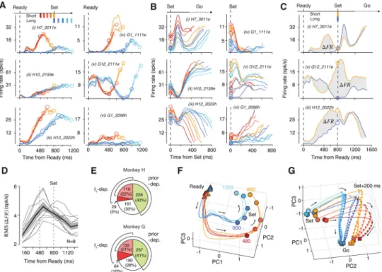
During the estimation epoch, many neurons had heterogeneous responses profiles that were modulated by elapsed time in a prior-dependent fashion (Figure 3A). Consequently,

responses at the time of Set varied with both the prior and ts (Figure 3B). The presentation of

Set triggered a transient modulation of firing rates (Figure 3B(i–iii,v)). Following this transient, neurons exhibited a range of monotonic (e.g., ramping) or non-monotonic

response profiles that were often organized according to ts irrespective of the prior condition

(Figure 3B(i–iii,vi)). Responses of many neurons during the Set-Go epoch were temporally scaled with respect to ts (i.e., stretched in time for longer ts), an effect that was most

conspicuous as a change of slope among the subset of ramping neurons (Figure 3B(ii,vi)). This temporal scaling is consistent with recent recordings in this area in a range of simple motor timing tasks (Emmons et al., 2017; Merchant et al., 2011; Mita et al., 2009; Remington et al., 2018a; Wang et al., 2018).

The influence of prior was most evident at the overlap ts of 800 ms (Figure 3C). Despite

identical task demands and temporal contingencies, many neurons had highly distinct firing rate patterns depending on the prior condition, with a maximum difference in firing rate during the support of the prior between 480 and 800 ms (Figure 3D). Remarkably, this effect

A

uthor Man

uscr

ipt

A

uthor Man

uscr

ipt

A

uthor Man

uscr

ipt

A

uthor Man

uscr

ipt

was present immediately after block transitions (Figure S2). We used a generalized linear model (GLM) to quantify the influence of ts and prior condition on spike counts (Figure 3E;

see Methods). Results indicated that approximately 30% of neurons were modulated by elapsed time (27% Monkey H, 31% Monkey G), and more than 60% were sensitive to the prior condition (65% Monkey H, 62% Monkey G). These results suggest that neural

responses during the support of the prior were shaped by a combination of the animal’s prior belief and the measured interval, which are the two key ingredients for computing the Bayesian estimate of ts.

Geometry and dynamics of population activity

The relationship between neurons with complex activity profiles and the computations they perform may be understood through population-level analyses that depict their collective dynamics as neural trajectories (Buonomano and Maass, 2009; Churchland et al., 2012; Fetz, 1992; Rabinovich et al., 2008; Remington et al., 2018b; Shenoy et al., 2013). Recent work has used this approach to elucidate neural computations in a wide range of motor and cognitive tasks (Carnevale et al., 2015; Hennequin et al., 2014; Mante et al., 2013; Michaels et al., 2016; Rajan et al., 2016; Remington et al., 2018a; Rigotti et al., 2010; Wang et al., 2018). Following this line of work, we sought to understand the computational principles of Bayesian integration in the RSG task by analyzing the population activity in DMFC. We applied principal component analysis (PCA) to study the evolution of neural trajectories for various experimental conditions. Our initial analysis indicated that neural responses associated with different effectors, target directions, and task epochs resided in different regions of the state space (Figure S4). Therefore, we applied PCA separately to neural responses across experimental conditions and task epochs. For all datasets, the population activity in each epoch was relatively low dimensional: 3–4 principal components (PC) in the estimation epoch and 5–10 PCs in the production epoch explained nearly 75% of total variance (Figure S3).

In the estimation epoch, neural trajectories associated with the two prior conditions were at different initial states at the time of Ready and became progressively more distinct

throughout their evolution (Figure 3F and S3; Movie S1). A notable feature of population activity in this epoch was the presence of curved neural trajectories during the support of each prior; i.e., approximately between 480 and 800 ms in the Short prior and between 800 and 1200 ms in the Long prior. The presence of this prior-specific curvature was consistent with responses of single neurons, many of which were selectively modulated during the support of each prior (Figure 3A(i,iii,iv)). This feature was ubiquitous for all experimental conditions (Figure S3), although the corresponding neural activity patterns resided in different parts of the state space (Figure S4).

The curved portion of the trajectories associated with the two prior conditions were parallel in the state space, suggesting that they relied on similar patterns of activity (Figure S4). Notably, the subspace for the 480 to 800 ms of the Short prior was shared to a greater extent with the subspace for the 800 to 1200 ms than the 480 to 800 ms of the Long prior (“Short In Long”; Figure S4). These findings are consistent with the observation that activity profiles of single neurons during the support of the prior were similar across the two prior conditions

A

uthor Man

uscr

ipt

A

uthor Man

uscr

ipt

A

uthor Man

uscr

ipt

A

uthor Man

uscr

ipt

(Figure 3A). These results highlight a potential link between the curvature and the neural representation of the prior.

In the production epoch, trajectories were at different initial states at the time of Set (Figure 3G, Movie S2). The Set flash caused a rapid displacement of neural states, after which neural states evolved toward a terminal state (Go) at a progressively slower rate for longer ts

(Figure 3G). The prior-dependent initial conditions, the Set-triggered transient response, and the ts-dependent rate of evolution of firing rates were all evident in the responses of many

single neurons (Figure 3B). Both the role of speed in the control of movement initiation time (Wang et al., 2018), and the importance of initial state in adjusting the speed (Remington et al., 2018a) have been demonstrated previously. The question that remains is how the brain establishes a sigmoidal mapping during the support of the prior so that the speed of the ensuing trajectories is appropriately biased according to Bayesian integration.

Bayesian estimation through latent dynamics

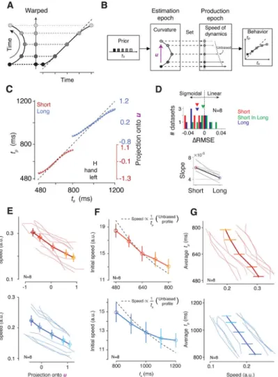
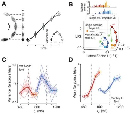
A property of a curved trajectory is that when projected onto a line connecting its two ends, equidistant points along the trajectory become warped. In other words, points near the ends of the projected line become biased toward the middle (Figure 4A), which qualitatively matches the sigmoidal mapping predicted from the Bayesian model (Figure 2). Based on this realization, we hypothesized that the curvature of neural trajectories during the support of the prior provides a computational substrate for Bayesian estimation. According to this hypothesis, which we refer to as the “curved manifold hypothesis”, the animal’s Bayesian behavior can be understood in terms of two computational stages (Figure 4B): 1) neural states evolving along the curved trajectory during the support of the prior provide an implicit, instantaneous representation of the Bayesian estimate of ts (te), and 2) this Bayesian

estimate adjusts the speed of the neural trajectory in the production epoch, which in turn, enables animals to optimally bias their responses.

1. Encoding Bayesian estimate along curved trajectory during prior support. —We asked whether projections of neural states along the curved trajectory onto a one-dimensional ‘encoding axis’ could establish a sigmoidal mapping similar to the Bayesian estimator (Figure 2A). Naturally, the answer depends on the choice of the encoding axis. Based on our understanding of the geometry of the problem (Figure 4A), we reasoned that a good candidate for the encoding axis is the vector pointing from the states associated with the shortest to the longest ts for each prior condition (u; Figure 4B). Neural projections onto

u exhibited biases that matched the Bayesian model fitted to the behavior (R2 _{= 0.993 for the}

Short prior, 0.996 for the Long prior; Figure 4C), and this match was specific to our choice of u (i.e., projection onto other randomly chosen vectors in the state space failed to produce a sigmoidal function, Figure S5). Indeed, the neural projections were better explained by the Bayesian model than a linear model for both priors (signed-rank test for RMSE, p=0.008 for the Short prior, p=0.008 for the Long prior; Figure 4D). As a negative control, we also analyzed neural data in the Long prior condition during a period temporally matched to support of the Short prior (“Short In Long” in Figure 4D) and found no evidence of sigmoidal representations (two-way repeated-measures ANOVA for RMSE with the prior

A

uthor Man

uscr

ipt

A

uthor Man

uscr

ipt

A

uthor Man

uscr

ipt

A

uthor Man

uscr

ipt

conditions and the models as factors, F1,7=161.43, p<10−5 for their interaction; post-hoc

signed-rank test between the Bayesian and linear models for Short In Long, p=0.74). A fundamental property of a Bayesian observer is that responses become more biased toward the mean of the prior when measurements are more uncertain (Figure 2G). As predicted, in the RSG task, we find larger behavioral biases for the Long prior condition (Figure 2H). Applying the same logic to the neural data, if projections onto the encoding vector represent te, they too should exhibit larger biases for the Long condition. A direct

comparison of projected neural states between the two priors was consistent with this prediction: the Long prior exhibited more bias than the Short prior as measured by slope of a regression line relating projections to ts (signed-rank test, p=0.008; Figure 4D). Together,

these results suggest that the curved trajectory in DMFC allow neural states to carry an implicit and instantaneous representation of te during the support of the prior.

2. Controlling speed based on Bayesian estimate during the Set-Go epoch.— Previous work has demonstrated that flexible production of timed intervals is made possible through adjustments of the speed at which neural trajectories evolve toward an action-triggering state (Afshar et al., 2011; Churchland et al., 2008; Hanes and Schall, 1996; Wang et al., 2018). Accordingly, the neural representations of te along the encoding axis should

serve as initial conditions to dictate the speed during the ensuing production epoch (Figure 4B). We therefore examined the relationship between speed and neural projections on the encoding axis within each prior condition. For both conditions, larger projections along the encoding axis were associated with slower speeds across all conditions (Figure 4E; Pearson correlation, ρShort=−0.74, p<10−7, ρLong=−0.51, p<10−3). Crucially, we also tested whether

speeds inherited biases from the warped organization of initial conditions at the time of Set. If Bayesian computation occurs during the support of the prior, speeds ought to incorporate the Bayesian biases immediately following Set. Accordingly, we computed the speed of neural trajectories early in the production epoch (i.e., initial speed) and examined the relationship between initial speed and ts. An unbiased speed profile predicts that the speeds

should be proportional to 1/ts. The speed profile for each prior condition, however,

demonstrated systematic biases with a central tendency: trajectories associated with shorter ts were slower than expected from an unbiased speed profile, and vice versa (Figure 4F;

Wilcoxon sign-rank test on measured versus unbiased regression slopes relating speed to ts,

p<10−3 combining conditions and animals). This biased speed profile is fully consistent with the pattern seen in the behavior. Finally, we verified that the overall speed of dynamics throughout the production epoch was predictive of the resulting tp across both priors and

across all experimental conditions (Figure 4G; Pearson correlation, ρShort=−0.58, p<10−4, ρLong=−0.52, p<10−3). Together, these results support the curved manifold hypothesis

according to which the curved trajectory supplies a Bayesian estimate of elapsed time, which controls the speed of dynamics during the production epoch allowing animals to produce Bayes-optimal behavior.

Alternative mechanisms

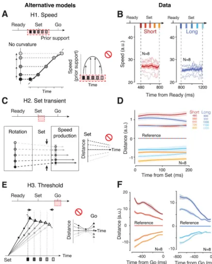
We considered three alternative mechanisms that could, in principle, establish a Bayesian sigmoidal mapping.

A

uthor Man

uscr

ipt

A

uthor Man

uscr

ipt

A

uthor Man

uscr

ipt

A

uthor Man

uscr

ipt

H1. Speed hypothesis: Bayesian integration through modulation of speed in the estimation epoch (Figure 5A).—One way to create a sigmoidal warping is to have neural states near the two ends of the prior evolve more slowly than near the prior mean. We tested this hypothesis by estimating the instantaneous speed of neural trajectories throughout the support of each prior. Results were not consistent with these predictions: for both prior conditions, speed remained unmodulated throughout the support of each prior (Figure 5b; signed-rank test for zero regression slopes during the support, p=0.64 for Short, p=0.08 for Long).

H2. Transient hypothesis: Bayesian integration by shaping the post-Set transient (Figure 5C).—Another way to create sigmoidal warping is to have the Set-triggered transient converge in the state space so as to elicit a bias in neural states toward the prior mean. To test this alternative, we computed the distance between neural trajectories during the first 200 ms following Set. Results indicated that neural trajectories for different ts in each prior evolved parallel to one another (signed-rank test for zero regression slopes

relating the distance to time after Set, p=0.92 for the shortest ts, p=0.13 for the longest ts,

across datasets and priors; Figure 5D; see also Figure 3G and S3). This suggests that the Set caused a ts-independent transient response in DMFC that did not contribute significantly to

the bias.

H3. Threshold hypothesis: Bayesian integration by establishing ts

-dependent movement thresholds (Figure 5E).—Finally, the biases could be induced by influencing the action-triggering state (i.e., threshold). If the threshold for fast trajectories (associated with shorter ts) is pushed further away, the neural trajectories would have to

travel a longer distance before reaching the action-triggering state, which would generate a positive bias. This model predicts, in particular, that states at the time of threshold-crossing should be different across ts, but more similar shortly before reaching the threshold due to

speed differences (Figure 5E left). The distance between neural trajectories should therefore decrease to a minimum before movement initiation, and increase again to reflect the ts

-dependent threshold at the time of Go (Figure 5E right). However, the distance profile of neural trajectories did not show this converging-diverging pattern; instead, the distance between trajectories appeared to drop steadily throughout the production epoch, even near the time of motor initiation (Figure 5F; one-tailed sign-rank test for time of minimum distance occurring strictly before movement initiation, p=1.5 × 10 −4, see Figure S5 for individual condition and animal).

The curved manifold hypothesis captures the variance of Bayesian estimates

Next we asked whether the curved manifold hypothesis could additionally account for the variance of te. According to the Bayesian model, the variance of te as a function of ts exhibits

an inverted-U shape (Figure 6A): the sigmoidal mapping causes estimates near the extrema of the prior to be more biased and less variable than estimates near the mean of the prior, which are unbiased but more variable.

From a geometrical standpoint, neural states projected onto the encoding axis would be able to readily capture this inverted-U pattern if a sizeable portion of variance across trials is

A

uthor Man

uscr

ipt

A

uthor Man

uscr

ipt

A

uthor Man

uscr

ipt

A

uthor Man

uscr

ipt

aligned to the curvature (Figure 6A). To test this possibility, we needed to derive accurate, trial-by-trial estimates of neural states. Such analysis is challenging but tractable if two conditions are concurrently met (Pandarinath et al., 2018; Williams et al., 2018; Yu et al., 2009): (1) data includes sufficiently large number of simultaneously recorded neurons, and (2) neural trajectories are governed by a small number of latent factors. Under these assumptions, Gaussian Process Factor Analysis (GPFA) can recover reliable estimates of single-trial neural trajectories (Afshar et al., 2011; Cowley et al., 2013; Yu et al., 2009). We therefore focused our analysis on high-yield sessions (N=48 for monkey H, N=107 for monkey G) and used GPFA to extract high-fidelity, single-trial neural trajectories for the estimation epoch. We projected the neural states at the time of Set onto the encoding axis, and computed the variance of the projections for each ts separately (Figure 6B; see

Methods). The resulting variance profile of single-trial projections resembled an inverted U-shape on average, with a tendency for lower variances at the extrema of each prior (one-tailed signed-rank test on coefficients for quadratic term in polynomial fitting, p=0.0273, Figure 6C; see Figure S6 for monkey G). This analysis indicates that the curved manifold hypothesis can additionally predict the second-order statistics of the Bayesian estimate. We also confirmed that the mean of the single-trial projections inferred from GPFA had a sigmoidal shape (signed-rank test between increments of mean Xu around extreme ts versus

those near middle ts, p=0.0078) and higher slope for the Short prior (one-tailed signed-rank

test for regression slope between Short and Long, p=0.0625; Figure 6D), consistent with results inferred from the trial-averaged firing rates (Figure 4C), and the behavior of the Bayesian estimator (Figure 2F,H). Finally, the single-trial neural state estimates derived from the GPFA analysis enabled us to validate the three-way relationship between neural states during the support of the prior (before Set), the speed of neural trajectories after Set, and the resulting tp (Figure S6).

Recurrent network models of cortical Bayesian integration

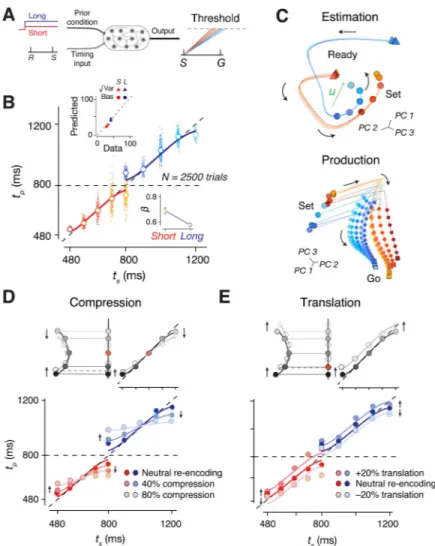
Recurrent neural network models (RNNs) have proven useful in elucidating how neural populations in higher cortical areas support various motor and cognitive computations (Mante et al., 2013; Rajan et al., 2016; Song et al., 2016; Sussillo et al., 2015; Yang et al., 2019). To gain further insight into how neural systems implement Bayesian inference, we trained RNNs to perform the two-prior RSG task (Figure 7A). On each trial, the network received a fixation cue as a tonic input whose value was adjusted by the prior condition. A second input administered the Ready and Set via two pulses that were separated by ts. The

network was trained to generate a linear ramping signal during Set-Go that would reach a fixed threshold (“Go”) at the correct time to reproduce ts. Using a suitable training strategy

(see Methods), we were able to build RNNs whose behavior was captured by a Bayesian observer model (Figure 7B).

Like DMFC neurons, RNN units displayed heterogeneous response profiles and were strongly modulated during the support of the prior (Figure S7). Similar to DMFC, the overall network activity was low dimensional during both the estimation and production epochs (Figure S7). Most importantly, network population trajectories exhibited the geometrical features of neural trajectories in DMFC. For instance, the network trajectories also exhibited

A

uthor Man

uscr

ipt

A

uthor Man

uscr

ipt

A

uthor Man

uscr

ipt

A

uthor Man

uscr

ipt

curvature during the support of the prior (Figure 7C and S7). Finally, during the production epoch, the initial condition and speed of trajectories were organized by ts (Figure 7C).

Next, we developed an on-manifold perturbation protocol to probe the causal link between the curved manifold and Bayesian integration. We allowed the network to evolve during the Ready-Set epoch, suspended the dynamics shortly before Set, placed the network into a desired altered state, and released the network to observe the effect of this perturbation on the behavior (see Methods for control experiments). The perturbation was designed to systematically displace neural states along the encoding axis – a strategy that we refer to as re-encoding. We reasoned that if indeed the curved manifold and the encoding vector u are responsible for warping neural representations of time, then perturbing the network state along the axis would lead to changes in behavior in a predictable manner.

Using this strategy, we perturbed the network activity in two ways: 1) compression along u toward the middle ts (mean of the prior), and 2) linear translation along u. According to our

hypothesis, the projection of activity along u provides an implicit representation for the Bayesian estimate of ts. The compression should therefore lead to increased bias toward the

mean ts (Figure 7D). The translation, on the other hand, should result in a systematic shift in

the values of tp towards longer or shorter intervals (Figure 7E) depending on the direction of

the translation. Results confirmed these predictions: tp values exhibited progressively larger

regression to the mean for larger compressive perturbations (Figure 7D), and underwent an overall upward or downward shift as a result of translation (Figure 7E). These in-silico experiments provide additional evidence for a potential causal role of the curved manifold in Bayesian computation.

Discussion

The central challenge in understanding Bayesian computations is the need for a framework that can bridge explanations across multiple scales. Most previous studies sought to understand Bayesian integration at the level of single neurons. This was also our starting point. We found that prior beliefs and sensory measurements concurrently modulated the firing rates of single neurons (Figure 3). Many previous studies have made similar

observations. For example, some studies found that the stochastic nature of spiking activity in single neurons could provide the means to implicitly encode sensory likelihoods (Jazayeri and Movshon, 2006; Ma et al., 2006). Others found that task-related firing rates of single neurons before the presentation of sensory information may be modulated by prior expectations (Basso and Wurtz, 1997; Rao et al., 2012), and firing rates after the

presentation of sensory information may reflect Bayesian estimate of behaviorally-relevant variables (Beck et al., 2008; Funamizu et al., 2016; Hanks et al., 2011; Jazayeri and Shadlen, 2015). There have also been attempts to apply reliability-weighted linear updating schemes – commonly used in cue combination studies (Angelaki et al., 2009; Fetsch et al., 2009; Gu et al., 2008) – to explain how single-neurons might combine sensory evidence with prior expectations (Darlington et al., 2018; de Xivry et al., 2013). Together, these results have provided valuable insights into single-neuron representations of prior beliefs and sensory measurements. However, probing the system at the level of single neurons has not led to a

A

uthor Man

uscr

ipt

A

uthor Man

uscr

ipt

A

uthor Man

uscr

ipt

A

uthor Man

uscr

ipt

principled understanding of the computational logic that populations of neurons implement to perform Bayesian integration.

To address this challenge, we investigated population neural activity using a framework that is rooted in the language of dynamical systems. The behavior of a dynamical system is constrained by the coupling between interacting variables in the system (Remington et al., 2018b). Recent theoretical studies have found that the same framework can be used to explain how synaptic coupling between neurons constrain the population activity pattern across a network of recurrently interacting neurons. In particular, it has been shown that structured connectivity in RNN models establishes low-dimensional manifolds with powerful computational capacities (Mastrogiuseppe and Ostojic, 2018) for integration (Wang, 2008), categorization (Chaisangmongkon et al., 2017), gating (Mante et al., 2013), timing (Goudar and Buonomano, 2018; Laje and Buonomano, 2013; Remington et al., 2018a; Wang et al., 2018), learning (Athalye et al., 2017; Golub et al., 2018; Sadtler et al., 2014), movement control (Gallego et al., 2017; Hennequin et al., 2014; Kaufman et al., 2014; Michaels et al., 2016; Shenoy et al., 2013; Sussillo et al., 2015) and forming

addressable memories (Hopfield, 1982). According to this framework, the computations that a neural system performs can be understood through an analysis of the geometry and dynamics of activity across the population (Gallego et al., 2017, 2018; Remington et al., 2018a; Sussillo, 2014).

Using this approach, we found a simple computational principle for how neural circuits perform Bayesian integration. We found that prior statistics that were presumably embedded in the coupling between neurons, established low-dimensional curved manifolds across the population. This curvature, in turn, warped the underlying neural representations giving rise to biased responses consistent with Bayes-optimal behavior. This mechanism was evident across multiple behavioral conditions including different prior distributions and different effectors suggesting that it may entail a general computational strategy for Bayesian integration.

Notably, the curved manifold not only explained the prior-dependent bias, but also

accounted for the drop in variance of single-trial Bayesian estimates near the extrema of the prior, consistent with the predictions of a Bayesian estimator. The fact that the variance of projected states as a function of ts exhibits an inverted-U shape suggests that a large fraction

of variability occurs along the trajectory (Figure 6A). This implies, in turn, that one of the main contributors of noise in the system might be the speed of the trajectory (Hardy et al., 2018; Mello et al., 2015; Wang et al., 2018).

This computational strategy also emerged in an RNN model trained on the same task. While previous work has demonstrated that artificial network models can perform a variety of sensory, motor, and decision-making tasks (Chaisangmongkon et al., 2017; Mante et al., 2013; Remington et al., 2018a; Wang et al., 2018; Yang et al., 2019), training networks to encode and integrate prior beliefs has remained a challenge. Relying on our understanding of the importance of signal-dependent noise in timing (Hardy et al., 2018; Mello et al., 2015; Wang et al., 2018), we were able to create a suitable training strategy that allowed the networks to integrate prior beliefs. In particular, we found that, among multiple training

A

uthor Man

uscr

ipt

A

uthor Man

uscr

ipt

A

uthor Man

uscr

ipt

A

uthor Man

uscr

ipt

regimes with different types of noises (see Methods), introduction of external noise mimicking scalar measurement variability was key to inducing the prior-dependent bias in the network.

One of the most highly sought-after advancements in systems neuroscience is an ability to exert full control over neural activity, which would allow the experimenter to investigate the behavioral and neural consequences of setting the population activity to a specific state (Jazayeri and Afraz, 2017). This is currently impossible because we do not have a technique that can adjust the firing rates of many neurons concurrently, although notable efforts in this direction have been made (Bashivan et al., 2019; O’Connor et al., 2013; Ponce et al., 2019). The possibility of such concurrent modification would be extremely valuable in further testing the merits of our curved manifold hypothesis, as it would allow us to validate whether neural states along the curved trajectory truly encode the animal’s internal estimates. Although it was not possible to perform this experiment in-vivo, establishing a recurrent neural network model of Bayesian integration allowed us to causally probe potential underlying mechanisms by performing such targeted population-level perturbations in-silico. The results of these experiments validated two key aspects of the curved manifold hypothesis: the orderly organization of the Bayesian estimates along the trajectory, and the role of the curvature in inducing regression toward the mean of the prior. Given the overall similarities of in-vivo and in-silico networks in terms of the response properties associated with Bayesian integration (Figure 7, S7), this causal validation of the mechanism in-silico provides tantalizing evidence that future experiments may find analogous results in-vivo. To put our findings in perspective, it is important to distinguish between the classic formulation of Bayes-optimal integration and the various algorithms the brain might use to optimize behavior in accordance with Bayesian theory. The classic formulation of Bayesian integration defines the likelihood function and prior probability distribution explicitly and uses them to compute a posterior distribution from which an optimal estimate can be inferred depending on a desired cost function. However, the derivation of optimal estimates from sensory measurements can be implemented by numerous isomorphic computational algorithms that do not necessarily depend on an explicit representation of the likelihood and/or the prior (Fiser et al., 2010; Ma and Jazayeri, 2014; Raphan and Simoncelli, 2006). Indeed, theoretical (Simoncelli, 2009) and behavioral (Acerbi et al., 2012; Jazayeri and Shadlen, 2010; Stocker and Simoncelli, 2006) studies have highlighted that Bayes-optimal behavior can be implemented by simple deterministic functions that map noisy measurement to optimal estimates. Our work supports this hypothesis; it shows that recurrent interactions between neurons establish manifolds whose geometry confers upon the population activity patterns an implicit representation of the optimal estimate without relying on explicit representations of the prior distribution and/or the likelihood function.

Although we focused on Bayesian integration in the domain of time, the key insights gleaned from our results may apply more broadly to perception, sensorimotor function, and cognition. For example, numerous studies have found an important role for natural scene statistics in vision and have shown that the organization of tuning in neurons of the primary visual cortex follow those statistics (Simoncelli and Olshausen, 2001). This observation is often explained in terms of efficient coding (Ganguli and Simoncelli, 2014; Simoncelli and

A

uthor Man

uscr

ipt

A

uthor Man

uscr

ipt

A

uthor Man

uscr

ipt

A

uthor Man

uscr

ipt

Olshausen, 2001). In this framework, neurons form heterogeneous basis sets that are tuned to the statistics of the environmental variables. In our timing task, we also found single neurons that developed flexible tuning for the support of each of the two priors (Figure 3). In other words, single neurons in our experiment also abided by the principles of efficient coding. However, our work goes beyond the representational notion of efficient coding and provides an understanding of how populations of neurons perform computations relevant to behavior. Our results suggest that statistical regularities in the environment create

geometrically constrained manifolds of neural activity that can suitably perform Bayesian integration.

STAR Methods

LEAD CONTACT AND MATERIALS AVAILABILITY

Further information and requests for resources and reagents should be directed to and will be fulfilled by the Lead Contact, Mehrdad Jazayeri (mjaz@mit.edu). This study did not

generate new unique reagents.

EXPERIMENTAL MODEL AND SUBJECT DETAILS

All experimental procedures conformed to the guidelines of the National Institutes of Health and were approved by the Committee of Animal Care at the Massachusetts Institute of Technology. Experiments involved two naive, awake, male behaving monkeys (species: M. mulatta; ID: H and G; weight: 6.6 and 6.8 kg; age: 4 yrs old). Animals were head-restrained and seated comfortably in a dark and quiet room, and viewed stimuli on a 23-inch monitor (refresh rate: 60 Hz). Eye movements were registered by an infrared camera and sampled at 1kHz (Eyelink 1000, SR Research Ltd, Ontario, Canada). Hand movements were registered by a custom single-axis potentiometer-controlled joystick whose voltage output was sampled at 1kHz (PCIe6251, National Instruments, TX). The MWorks software package (http:// mworks-project.org) was used to present stimuli and to register hand and eye position. Neurophysiology recordings were made by 1–3 24-channel laminar probes (V-probe, Plexon Inc., TX) through a bio-compatible cranial implant whose position was determined based on stereotaxic coordinates and structural MRI scan of the two animals. Analysis of both behavioral and spiking data was performed using custom MATLAB code (Mathworks, MA). METHOD DETAILS

Two-prior time-interval reproduction task

Task contingencies.: Animals were trained on an interval-timing task that we refer to as the Ready-Set-Go (RSG) in which they had to measure a sample interval, ts, and produce a

matching interval tp by initiating a saccade or by moving a joystick. Each experimental

session consisted of 8 randomly interleaved conditions, 2 effectors (Hand and Eye), 2 movement targets (Left and Right), and 2 prior distributions of ts (Long and Short).

Trial structure.: Each trial began with the presentation of a circle (diameter: 0.5 deg) and a square (side: 0.5 deg) immediately below it. Animals had to fixate the circle and hold their gaze within 3.5 deg of it. The square instructed animals to move the joystick to the central location. To aid the hand fixation, we briefly presented a cursor whose instantaneous

A

uthor Man

uscr

ipt

A

uthor Man

uscr

ipt

A

uthor Man

uscr

ipt

A

uthor Man

uscr

ipt

position was proportional to the joystick’s angle and removed it after successful hand fixation. Upon successful fixation and after a random delay (500 ms plus a random sample from an exponential distribution with mean of 250 ms), a white movement target was presented 10 deg to the left or right of the circle (diameter: 0.5 deg). After another random delay (250 ms plus a random sample from an exponential distribution with mean of 250 ms), the Ready and Set stimuli were flashed sequentially around the fixation cues (outer

diameter: 2.2 deg; thickness: 0.1 deg; duration: 100 ms). The animal had to measure the sample interval, ts, demarcated by Ready and Set, and produce a matching interval, tp, after

Set by making a saccade or by moving the joystick toward the movement target presented earlier (Go). Across trials, ts was sampled from one of two discrete uniform prior

distributions, each with 5 equidistant samples, a “Short” distribution between 480 and 800 ms (µShort = 640 ms, σ2Short = 8533 ms2), and a “Long” distribution between 800 and 1200

ms (µLong = 1000 ms, σ2Long = 13333 ms2).

The 4 conditions associated with the 2 effectors and 2 prior conditions were interleaved randomly across blocks of trials. For 15 out of 17 sessions, the block size was set by a minimum (3 and 5 trials for H and G, respectively) plus a random sample from a geometric distribution with a mean of 3 trials that was capped at a maximum (20 for H and 25 for G). The resulting mean ± SD block lengths were 4.0 ± 4.4 and 13.3 ± 3.1 trials for H and G, respectively. In 2 sessions in H, switches occurred on a trial-by-trial basis. Because animal G had more trouble switching between conditions, block switches involved a change of prior or effector but not both. The position of the movement target was randomized on a trial-by-trial basis. Throughout every trial, the fixation cue provided information about the underlying prior and the desired effector. One of the two fixation cues was colored and the other one was white. The animal had to respond with the effector associated with the colored cue (circle for Eye and square for Hand), and the cue indicated the prior condition (red for Short and blue for Long).

To receive reward, animals had to move the desired effector in the correct direction, and the magnitude of the relative error defined as |t_p− t_s| /t_s had to be smaller than 0.15. When rewarded, reward decreased linearly with relative error, and the color of the response target changed to green. Otherwise, no reward was given and the target turned red. Trials were aborted when animals broke the eye or hand fixation prematurely before Set, used incorrect effector, moved opposite to the target direction, or did not respond within 3ts after Set. To

compensate for lower expected reward rate in the Long prior condition due to longer duration trials (i.e., longer ts values), we set the inter-trial intervals of the Short and Long

conditions to 1220 ms and 500 ms, respectively. Electrophysiology

Recording.: We recorded from 617 and 741 units in monkey H and G, respectively in the dorsomedial frontal cortex (DMFC), comprising supplementary eye field (SEF),

presupplementary motor area (Pre-SMA), and dorsal portion of the supplementary motor area (SMA). No recordings were made in the medial bank. Regions of interest were selected according to stereotaxic coordinates with reference to previous studies recording from the SEF (Fujii et al., 2002; Huerta and Kaas, 1990; Schlag and Schlag-Rey, 1987; Shook et al.,

A

uthor Man

uscr

ipt

A

uthor Man

uscr

ipt

A

uthor Man

uscr

ipt

A

uthor Man

uscr

ipt

1991) and Pre-SMA (Fujii et al., 2002; Matsuzaka et al., 1992), and the existence of task-relevant modulation of neural activity. Recorded signals were amplified, bandpass filtered, sampled at 30 kHz, and saved using the CerePlex data acquisition system (Blackrock Microsystems, UT). Spikes from single-units and multi-units were sorted offline using Kilosort software suites (Pachitariu et al., 2016). We collected 456 single-units (H:196, G: 260) and 902 multi-units (H:421, G:481) in 69 penetrations across 29 sessions (H:17, G:12). QUANTIFICATION AND STATISTICAL ANALYSIS

Analysis of behavior

Model free analysis of behavior.: We analyzed behavior in sessions with simultaneous neurophysiological recordings (H: 17 sessions, 26189 trials, G: 12 sessions, 30777 trials). First, we used a probabilistic mixture model to exclude outliers from further analysis. The model assumed that each tp was either a sample from a task-relevant Gaussian distribution or

from a lapse distribution, which we modeled as uniform distribution extending from the time of Set to 3ts. We fit the mean and standard deviation of the Gaussian for each unique

combination of session, prior condition, ts, effector, and target directions. Using this model,

we excluded any trial in which tp was more likely sampled from the lapse distribution

(3.84% trials in H and 5.7% trials in G).

We measured the relationship between tp and ts separately for each combination of prior,

effector, and target direction in individual sessions using linear regression (t_p= βt_s+ ε). Since tp is more variable for larger ts due to scalar variability, we used a weighted regression;

i.e., error terms for each ts were normalized by the standard deviation of the distribution of tp

for that ts. We tested whether regression slopes were larger than 0 and less than 1 (Figure 1

and S1, Table S1).

Analysis of behavior with a Bayesian model.: We fit a Bayesian observer model to behavioral data (Figure 2). The Bayesian observer measures ts using a noisy measurement

process that generates a variable measured interval, tm. The measurement noise has a

Gaussian distribution with a mean of zero and a standard deviation that scales with ts with

constant of proportionality wm. The observer combines the likelihood function, p(tm|ts), with

the prior, p(ts), and uses the mean of the posterior, p(ts|tm), to compute an estimate, te. For a

uniform prior, and under scalar property of time measurements, the mapping between te and

tm is sigmoidal (Figure 2). The observer aims to produce te through another noisy process

generating a variable tp. We assumed that production noise scales with te with constant of

proportionality wp. For each prior, the model also included an offset term (b) to

accommodate any overall bias in tp. Using maximum likelihood estimation (MLE), we fit

the 4 free parameters of the model (wm, wp, bShort, and bLong) to data for each animal,

effector, and target directions after pooling across sessions (Table S3).

Analysis of single- and multi-unit activity—Most analyses were performed in a condition-specific fashion (2 priors, 5 ts per prior, 2 effectors, and 2 directions). We excluded

units for which we had less than 5 trials per condition, and units whose average firing rate was less than 1 spike/s. The remaining units included in subsequent analyses were 536 and 636 in H and G, respectively. To plot response profile of individual neurons (Figure

A

uthor Man

uscr

ipt

A

uthor Man

uscr

ipt

A

uthor Man

uscr

ipt

A

uthor Man

uscr

ipt

3A,B,C), we smoothed averaged spike counts in 1-ms bins using a Gaussian kernel with a standard deviation of 25 ms.

Generalized linear model.: We used a generalized linear model (GLM) to assess which neurons were sensitive to the prior and ts. We modeled spike counts in an 80-ms window

immediately before Set, rSet, as a sample from a Poisson process whose rate was determined

by a weighted sum of a binary indicator for prior (Iprior: 1 for Long, 0 for Short) and 5

binary indicators for ts values (Its) associated with the Short prior for which we also knew

the firing rate for the Long prior. The model was augmented by 2 additional binary indicators to account for independent influences of the effector (Ieffector: 1 for Hand, 0 for

Eye), and direction (Idirection:1 for Left, 0 for Right).

r_set= 5_{j = 1}β_tsI_ts(j) + β_priorI_prior+ β_{e f f ector}I_{e f f ector}+ β_directionI_direction

Equation 1

To get the most reliable estimate for the regression weights, we included spike counts based on all trials with attrition (i.e., firing rate at time t was computed from spikes in all trials in which Set occurred after t), and estimated β parameters of the model using MLE for all included neurons. To assess the significance of the effect of the prior condition, we used Bayesian information criteria (BIC) to compare the full model (Equation 1) to a reduced model that did not include a regressor for the prior (Equation 2):

r_set= 5_{j = 1}β_tsI_ts(j) + β_{e f f ector}I_{e f f ector}+ β_directionI_direction

Equation 2

We also used a GLM to assess which neurons were sensitive to ts. Since values of ts were

different between the priors, we used two distinct GLMs, one for data in the Short prior and one for the Long prior (Equation 3):

r_set= 5_{j = 1}β_tsI_ts(j) + β_{e f f ector}I_{e f f ector}+ β_directionI_direction

Equation 3

Equation 3 has the same format as Equation 2 but was used to assess neural data in the two prior conditions separately. To identify the neurons that were sensitive to ts, we used BIC to

compare the ts-dependent GLM (Equation 3) to a reduced GLM in which there was no

sensitivity to ts (Equation 4):

A

uthor Man

uscr

ipt

A

uthor Man

uscr

ipt

A

uthor Man

uscr

ipt

A

uthor Man

uscr

ipt

r_set= β₀+ β_{e f f ector}I_{e f f ector}+ β_directionI_direction

Equation 4

Neurons were considered ts-dependent if the BIC was lower in the full model either for the

Short or for the Long prior condition (Figure 3). Analysis of population neural activity

Principal component analysis.: To examine the trajectory of population activity in state space, we applied principal component analysis (PCA) to condition-specific, trial-averaged firing rates (bin size: 20 ms, Gaussian smoothing kernel width: 40 ms). Since neurons modulated during estimation and production epochs were largely non-overlapping (Figure S4), we performed PCA separately on the two epochs. We first constructed firing rate matrices of all neurons and time points [time points × neurons]. This yielded 16 matrices (2 priors × 2 effectors × 2 directions × 2 epochs). We then concatenated the matrices across the two prior conditions along the time dimension and applied PCA to each of the resulting 8 data matrices to find principal components (PCs) for each unique combination of effector and direction, separately in the two epochs.

In the estimation epoch, firing rates for each ts were estimated with attrition (i.e., firing rate

at time t was computed from spikes in all trials in which Set occurred after t). However, results were qualitatively unchanged if firing rates were estimated without attrition. In the production epoch, to accommodate different trial lengths (i.e., variable tp), we estimated

firing rates only up to the shortest tp for each ts. Neural trajectories in the two epochs were

analyzed within the subspace spanned by the top PCs that accounted for at least 75% of total variance (Figure S3). We will use X(t) to refer to a neural state within the PC space at time t. Analysis of neural projection.: In the estimation epoch, we examined the curvature in neural trajectories during the support of each prior by projecting X(t) onto an ‘encoding axis’, u, defined by a unit vector connecting the state associated with the shortest ts (ts_min)

to that with the longest ts (ts_max) for that prior. We denote the projected states by Xu. To

reduce estimation error, we computed multiple difference vectors connecting X(ts_min+Δt) to

X(ts_max-Δt) for every Δt=20 ms, and used the average as our estimate of u. We used

bootstrapping (resampling trials with replacement 1000 times) to compute 95% confidence interval for Xu. We quantified the similarity between Xu and the Bayesian estimates (te)

inferred from model fits to behavior using linear regression (Xu = α + βt_e). Since we included spike counts across trials with attrition, there were nearly 5 times more data for the shortest t_s compared to the longest t_s within each prior. Accordingly, for each t_s, error terms were weighted by the number of data points included for that ts (5 for the shortest ts, 4 for

the second shortest, and so forth). We then used the coefficient of determination (R2) to assess the degree to which te was explained by the neurally inferred Xu. To further validate

the warping hypothesis that Xu encodes te, we tested whether any linear model of ts (Xu = α

A

uthor Man

uscr

ipt

A

uthor Man

uscr

ipt

A

uthor Man

uscr

ipt

A

uthor Man

uscr

ipt

+ βts) can fit Xu better. The number of free parameters (α, β) were matched between the

Bayesian and linear models as te was computed only from behavioral data. The model fit

was compared in terms of Root Mean Squared Error (RMSE) between the actual and predicted Xu for individual datasets (2 animals × 2 effectors × 2 directions). As a negative control of our analysis, we applied the same projection analysis to data of the Long prior from 480 ms to 800 ms after Ready, which corresponded to the support of the Short prior (‘Short In Long’). We also compared the slope β for ts between the two prior conditions

(Figure 4D) as we performed in the behavioral analysis (Figure 2G, H). Finally, we tested the specificity of our results with respect to the chosen u by performing the same analysis for 1000 randomly chosen encoding axes (u’), and comparing the corresponding R2 _values

(Figure S5).

We examined two later links of the cascade model (Figure 4B) during the production epoch. A key component in the production epoch was the speed of the neural trajectory travelling the state space. For each dataset, we computed the speed as the average Euclidean distance (in the PC space accounting for at least 75% of the total variance) between neural states associated with successive bins (20 ms), divided by the duration separating Set and the time of Go. First, we related the trajectory speed to the projected state along the encoding axis (u) across the prior and ts to test if the state served as an initial condition to set up the speed of

the ensuing trajectory (Figure 4E). We then assessed how the speed during the production epoch was associated with the behavioral output, tp (Figure 4G). We computed a correlation

coefficient between the tp averaged across trials of each dataset and the trajectory speed and

tested its statistical significance (p<0.05).

Test of alternative mechanisms.: To test alternative neural models for generating bias (Figure 5), we focused on two main features of neural trajectories: speed and distance across trajectories of the different priors and t_s. We applied PCA as before but only to the period of interest for each alternative model (from Set to Set+200 ms for the ‘Set transient model’, from Go-800 ms to Go for the ‘Threshold model’). For the ‘Speed model’, we estimated instantaneous speed of the trajectory in the full neural space to avoid any potential distortion by smoothing and PCA (Figure 5B). For distance metric, trajectory of the middle t_s (i.e. prior mean) was used as a reference from which the distance was computed (Figure 5D,F). Analysis of neural state variance.: To estimate variance of neural states across individual trials during the support of the prior (Figure 6A), we used the following procedure. 1) We estimated the single-trial neural trajectories by applying Gaussian Process Factor Analysis (GPFA) (Cowley et al., 2013; Yu et al., 2009) to data from simultaneously recorded neurons in a single session (N= 48 in H, 96 in G) with cross validation. GPFA allowed us to avoid arbitrarily selecting size of the smoothing kernel and to estimate shared variability across population of neurons. 2) We projected the single-trial states onto the encoding vector (u) (Figure 6B). 3) We calculated variance and mean of the neural projections for each ts in each

prior condition. We also used GPFA to obtain single-trial estimate of the trajectory speed during the production epoch. We examined correlation between the trial-by-trial speed and the neural projection (Figure S6) and correlation between the speed and tp across trials

(Figure S6). To ensure that our analysis correctly captured the trial-by-trial relationship

A

uthor Man

uscr

ipt

A

uthor Man

uscr

ipt

A

uthor Man

uscr

ipt

A

uthor Man

uscr

ipt

between speed and tp and not their co-dependence on ts (Figure 4E,G), we measured

correlations after z-scoring single-trial data for each ts, and used the total-least squares

algorithm to ensure that the estimation errors of both speed and tp were taken into account.

Recurrent neural network—We constructed a randomly connected firing-rate recurrent neural network (RNN) model with N = 200 nonlinear units. The network dynamics were governed by the following equations:

τx˙(t) = − x(t) + Jr(t) + Bω(t) + c_x+ ρ_x(t)

Equation 5

r(t) = tanh(x(t))

Equation 6

x(t) is a vector containing the activity of all units and r(t) represents the firing rates of those units, obtained by a nonlinear transformation of x. Time t was sampled every millisecond for a total duration of T = 3500 ms. The time constant of decay (τ) for each unit was set to 10 ms. The unit activations also contain an offset cx and white noise ρx(t) sampled at each time

step from zero-mean normal distributions with standard deviation lying in the range between 0.01 and 0.015. The matrix J represents recurrent connections in the network. The network received multi-dimensional input ω through synaptic weights B = [bc, bs]. The input

comprised of a prior-dependent context cue ωc(t) and an input ωs(t) that provided Ready and

Set pulses. In ωs(t) Ready and Set were encoded as 20 ms pulses with a magnitude of 0.4

that were separated by time tm, where t_m∼ N(t_s, t_sw_m). wm represents the weber fraction by

which the noise process scales. The amplitude of the prior-dependent context input ωc(t) was

set to 0.3 for the Short prior and 0.4 for the Long prior contexts. Networks produced a one-dimensional output z(t) through summation of units with weights wo and a bias term cz.

z(t) = w_oTr(t) + c_z

Equation 7

Network Training.: Prior to training, model parameters (θ), which comprised J, B, wo, cx,

and cz were initialized. Initial values of matrix J were drawn from a normal distribution with

zero mean and variance 1/N, following previous work (Rajan and Abbott, 2006). Prior to training, synaptic weights B and the initial state vector x(0) and unit biases cz were drawn

A

uthor Man

uscr

ipt

A

uthor Man

uscr

ipt

A

uthor Man

uscr

ipt

A

uthor Man

uscr

ipt

from a uniform distribution with range [−1,1]. The output weights, wo and bias cz were

initialized to zero. During training, model parameters were optimized by truncated Newton methods (Martens and Sutskever, 2012) using backpropagation-through-time (Werbos, 1990) by minimizing a squared loss function between the network output zi(t) and a target

function fi(t), as defined by:

H(θ) = 1_T

trI I Ttr(zi(t) − fi(t))

2

Equation 8

Here i indexes different trials in a training set (I = different prior contexts × intervals (ts) ×

repetitions (rc)). Ttr represents the epoch within a trial that was used to compute H(θ) and

here corresponds to the production epoch. Accordingly, the target function fi(t) was only

defined in the production epoch. The value of fi(t) was zero during the Set pulse. After Set,

the target function was governed by two parameters that could be adjusted to make fi(t)

nonlinear, scaling, non-scaling or approximately-linear:

f_i(t) = A(e

t αts_{− 1)}

Equation 9

For the networks reported, fi(t) was an approximately-linear ramp function parametrized by

A = 3 and α = 2.8. Solutions were robust with respect to the parametric variations of the target function (e.g., nonlinear and non-scaling target functions). In trained networks, tp was

defined as the time between the Set pulse and when the output ramped to a fixed threshold (zi = 1).

During training, we employed three strategies to obtain robust solutions. In general, we injected three sources of variability: (1) Noise added to individual units in the RNN, (2) noise added to input, and (3) noise imposed by jittering the time of events (scalar

variability). The third regime generated the most Bayes-consistent results. In this scheme, the RNNs were trained such that interval-dependent scalar noise was introduced into their observations (various trials t_m∼ N(t_s, t_sw_m)); however, the target was always held to be the mean of those likelihood functions (t_s). In other words, interval between the Ready and Set pulses varied across trials with the scalar noise (t_m) while the network was trained to generate a ramping output during the production epoch that would reach threshold at Set+ t_s. Within this family of networks, we systematically varied two parameters (repeated across multiple networks), w_m (weber fraction of the scalar noise) and the variance of white noise added to individual units to regularize the training procedure. However, it was challenging to train networks under such scalar noise. Complete failure of training was common and only

A

uthor Man

uscr

ipt

A

uthor Man

uscr

ipt

A

uthor Man

uscr

ipt

A

uthor Man

uscr

ipt