HAL Id: tel-02524279
https://tel.archives-ouvertes.fr/tel-02524279
Submitted on 30 Mar 2020HAL is a multi-disciplinary open access archive for the deposit and dissemination of sci-entific research documents, whether they are pub-lished or not. The documents may come from teaching and research institutions in France or abroad, or from public or private research centers.
L’archive ouverte pluridisciplinaire HAL, est destinée au dépôt et à la diffusion de documents scientifiques de niveau recherche, publiés ou non, émanant des établissements d’enseignement et de recherche français ou étrangers, des laboratoires publics ou privés.
Learning Multimodal Digital Models of Disease
Progression from Longitudinal Data : Methods &
Algorithms for the Description, Prediction and
Simulation of Alzheimer’s Disease Progression
Igor Koval
To cite this version:
Igor Koval. Learning Multimodal Digital Models of Disease Progression from Longitudinal Data : Methods & Algorithms for the Description, Prediction and Simulation of Alzheimer’s Disease Pro-gression. Other Statistics [stat.ML]. Institut Polytechnique de Paris, 2020. English. �NNT : 2020IP-PAX008�. �tel-02524279�
574
NNT
:
2020IPP
AX008
Learning Multimodal Digital Models
of Disease Progression from
Longitudinal Data:
Methods & Algorithms for the Description,
Prediction and Simulation of Alzheimer’s
Disease Progression.
Thése de doctorat de l’Institut Polytechnique de Paris préparée á Ecole Polytechnique Ecole doctorale n◦574 Ecole Doctorale de Mathématiques
Hadamard (EDMH)
Spécialité de doctorat: Mathématiques Appliquées
Thèse présentée et soutenue à Paris, France, le 23 Janvier 2020, par
I
GORK
OVALComposition du Jury :
Daniel Alexander
Professeur, University College London Rapporteur
Sach Mukherjee
Professeur associé, DZNE Rapporteur
Martin Hofmann-Apitius
Professeur, Fraunhofer SCAI Examinateur
Erwan Le Pennec
Professeur, Ecole Polytechnique Président
Stéphanie Allassnnière
Professeur, Université Paris-Descartes Co-directrice de thèse
Stanley Durrleman
Directeur de Recherche, Inria Co-directeur de thèse
Stéphane Epelbaum
Abstract
This thesis focuses on the statistical learning of digital models of neurodegenerative dis-ease progression, especially Alzheimer’s disdis-ease. It aims at reconstructing the complex and heterogeneous dynamic of evolution of the structure, the functions and the cognitive abilities of the brain, at both an average and individual level. To do so, we consider a mixed-effects model that, based on longitudinal data, namely repeated observations per subjects that present multiple modalities, in parallel recombines the individual spatiotem-poral trajectories into a group-average scenario of change, and, estimates the variability of this characteristic progression which characterizes the individual trajectories. This vari-ability results from a temporal un-alignment (in term of pace of progression and age at disease onset) along with a spatial variability that takes the form of a modification in the sequence of events that appear during the course of the disease. The 5 parts of this thesis corresponds to different aspect and features that extensively enrich the initial statistical model in order to convert it into a natural framework for the study of disease progression. The first part of the manuscript aims at presenting the generative mixed-effects model that enables the estimation of the long-term progression of the disease and to reconstruct the individual trajectory, in the case of multivariate data. It offers a generic way to handle individual spatiotemporal trajectories that present a natural variability between patients. This variability results from a temporal un-alignment (different pace of progression and a temporal offset) along with a spatial variability that takes the form of a modification in the sequence of events that appear during the course of the disease.
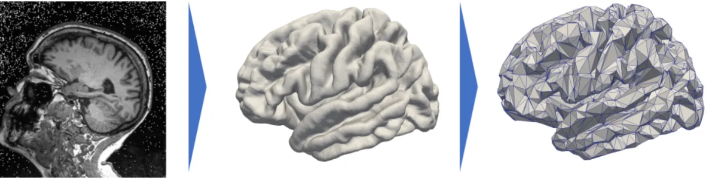
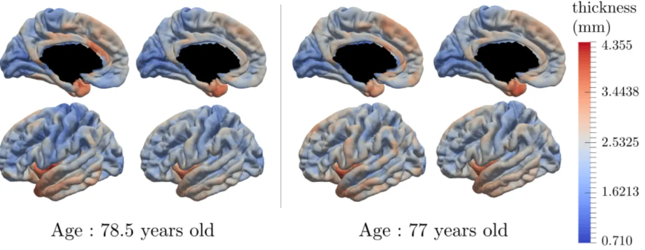
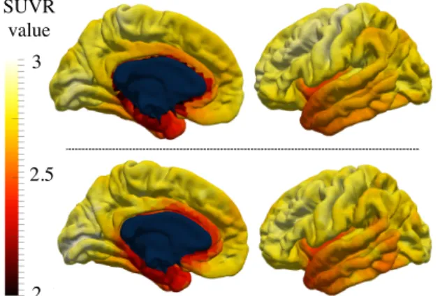
The second part expands the scope of the model in order to handle data that have a spatial structure, such as images, meshes and networks. It introduces a technique to take advantage of the spatial coherence of evolution for close regions. It is validated on the estimation of the cortical thickness and glucose consumption evolution during the course of Alzheimer’s disease.
The third part is an extensive study of the complex progression of the function (FDG-PET), the structure (cortical thickness and hippocampus meshes) and cognitive abilities (ADAS-Cog and MMSE) during the course of Alzheimer’s disease. It validates the group-average multi-modal progression, evaluated by the reconstructing of individual trajectories to the noise level. The analysis of the factors modulating the evolution enables to describe the interactions between heterogeneous modalities. Furthermore, it allows to predict indi-vidual measurements up to 4 years in advance.
The fourth chapter takes advantage of the generative and mixed-effects nature of the model. It offers the possibility to first reconstruct a continuous disease timeline at the individual level and also to simulate virtual patients entirely. The former allows to impute missing values or predicting future time-points. The latter enables to simulate virtual patients that either un-bias and balance the real cohort or to augment the initial dataset in order to improve the predictive power of algorithms that requires large amount od data. It is used to reach state-of-the-art results on future stages 3 and 4 years in advance.
The fifth chapter describes the software tools that were developed along the way. They were designed to benefit to mathematical researchers that aims to develop similar models or estimation algorithms, while being sufficiently user-friendly to be used by the medical community for other diseases or even in real-life disease diagnosis and prognosis.
To conclude, this thesis introduces a general framework to grasp the complexity of the disease progression in inter-dependant heterogeneous modalities. Overall, this advanced understanding enables to characterize individual evolutions, simulate virtual cohorts and predict future disease stages for various modalities. While it focuses on the study of Alzheimer’s disease solely, current works on Parkinson’s disease, Huntington’s disease and normal ageing highlights its capacity to generalize to other neurodegenerative diseases.
Remerciements
Il est des expériences de vie dont on ne ressort grandit que si l’on en vient à bout seul. A l’inverse, certaines acquièrent leur saveur au contact des lieux, des discussions et des personnes qui les ont vues naître et grandir. Cette thèse en a été une illustration manifeste ; elle est l’aboutissement d’une initiation intellectuelle unique et inattendue, dont le parcours a été embelli par des rencontres inestimables, et soutenu par un soutien amical et familial indéfectibles.
Mes remerciements s’adressent d’abord à Sach Mukherjee et Daniel Alexander pour avoir accepter de relire mon manuscript de thèse. Leurs rapports, traduisant l’attention qu’ils ont su porter à ce travail, ont été précieux pour en mettre en valeur certains aspects. Aussi, j’adresse toute ma gratitude à Martin Hofmann-Apitius et Erwan Le Pennec que j’ai eu la joie de compter parmi les membres de mon jury.
Ensuite, ce sont à mes directeurs de thèse, Stéphanie Allassonnière et Stanley Dur-rleman, que sont dédiés ces mots. Mes pensées pour eux ne sauraient décrire la joie que j’ai eu à travailler sous leur tutelle. Sans eux, ce travail n’aurait que peu des qualités, s’il en est, qui le traversent aujourd’hui : scientifiques, rédactionelles, pédagogiques, ... Leurs conseils ont fait de l’exercice que constitue une thèse, un travail passionnant et passionné. Au delà de mes directeurs de thèse, Aramis a été un laboratoire scientifique extraordi-naire. Ce lieu, ironiquement situé entre la morgue et la maternité, a été bien plus qu’un lieu de travail ; un lieu de vie, de découverte et d’épanouissement. Olivier Colliot, directeur du laboratoire, bienveillant et sincère, toujours disposé à livrer son avis éclairé, sans qui cette équipe ne serait telle qu’elle est. Emmanuelle, dont la gentillesse a apporté un brin d’humanité et de douceur au milieu de tous ces scientifiques. Ninon et Fabrizio, dont les récentes récompenses prouvent leurs grandes qualités scientifiques, mais aussi humaines. Stéphane pour qui j’ai le plus profond respect ; professionnel, d’abord, des consultations qui m’ont fait entrevoir toute l’empathie et l’altruisme du docteur, mais personnel, surtout. Enfin, une pensée pour Anne, dont le sourire nous manque toujours.
S’ajoute à ces membres, les doctorants et ingénieurs, qui, bien que de passage, auront écrit une page de l’histoire d’Aramis et de mon séjour en son sein. Mes aînés d’abord. Jean-Baptiste qui a su me transmettre ses travaux avec beaucoup de bienveillance. Hao, Catalina, Jérémy, Jorge et Alexandre R., qui en plus de nous montrer la voie scientifique, ont été des collègues et amis précieux, et pour certains, des danseurs hors pair. Mes contemporains ensuite, grâce a qui cette thèse a été un travail exaltant et collectif. Manon, rigoureuse, dédiée à son travail et ses principes, inspirante par son dévouement. Maxime, qui, en plus d’être un compagnon scientifique - et de cordée - a surtout été un complice intellectuel sur tous les sujets sociaux et sociétaux. Alexandre B., qui aura été le trublion de l’équipe, l’infatigable animateur de nos discussions et de nos pauses, à EuroPOND comme ailleurs. Juliette me fascinant par son éternel intérêt pour les convergences théoriques -plus que pratiques. Enfin, à la -plus jeune génération. Celle qui me rappelle qu’en trois ans à peine, mon statut d’ancien du labo a à jamais remplacé celui de jeune doctorant. Tiziana, pour représenter haut et fort les couleurs de l’Italie et du sourire romain, inébranlable, du matin au bout de la nuit. Raphael, avec qui les sorties n’ont jamais été aussi étonnantes et sensationnelles - au propre comme au figuré. Simona, d’abord pour l’irrésistible plaisir qu’elle aura à ouvrir ces pages pour y trouver son nom. Mais par dessus tout, sa bonne humeur, surtout lorsqu’elle s’exprime par une tâche de café, de dentifrice ou de ketchup. Et pour toutes les discussions de canapé, de bar et à travers les vitres que nous avons eues et auront encore. Arnaud M. pour toutes les sensations fortes que nous avons pu partager, de jour comme de nuit.
Écrire ces lignes me rapelle que ces mots sont adressés à des amis avant tout. Cette thèse et la vie qui l’a accompagnée m’apparaissent maintenant comme des moments de
vie exceptionnels, sans précédents. Principalement liés aux personnes qui m’entourent, et dont j’essaye de tirer le meilleur enseignement, par nos discussions animés, leurs opinions et nos aventures: Paris, Québec, Florence, Barcelone, Londres, Rotterdam, ...
Le soutien de mes amis a également été précieux pendant ces années de thèse. De mes années d’études aux Ponts me reste des amis chers, et dont les réussites personnelles et professionnelles ont été inspirantes pour mes propres décisions. S’y ajoute le groupe des prépas ou des troubadours comme il me plaisait de les appeler. Ce quolibet fut en réalité la raison de mon attachement à eux, puisqu’ils se distinguent par leurs métiers, éloignés du mien, qui me rappelle la pluralité des avis, des opinions et des visions du monde. Enfin mes amis les plus anciens, du lycée comme nous avons coutumes de nous appeler, bien que la plupart de ces amitiés remontent à nos balbutiements de collégiens. Les remercier tous serait tâche déraisonnée. Mais les liens qui nous rassemblent sont d’autant plus fascinants qu’ils tiennent à nos différences, tant professionnelle, qu’idéologique, culturelle, ...
Enfin, aucune des étapes de ma vie, à l’aune de ces remerciements, n’aurait existé sans les efforts, l’assistance et les conseils déterminants que m’ont apporté ma famille. Cathy et Pascal, qui ont grandement participé à mon éducation, m’ont conseillé infailliblement. A Monique, qui n’a jamais lésiné sur les efforts. Pour me faire réciter mes leçons, dès le début. Pour inspirer et motiver mes décisions scolaires. Et pour toutes ces choses qu’elle m’a toujours affectueusement apportées. Et enfin, à mes parents, Irena et Oleg. Leurs efforts, leur invariable soutien, apportés pendant ma toute ma scolarité, sans jamais m’en faire sentir le poids, pour m’accompagner coute que coute. J’espère que la fierté qu’ils tireront de mon travail saura prouver l’amour que je leur porte. S’y ajoute une pensée particulière à ma famille en Ukraine, dont j’espère que cette thèse aura rendu fier, malgré la distance qui nous sépare.
Enfin, ce travail ne serait ce qu’il est sans celle qui accompagne mes joies et mes peines depuis tant d’années. Bien qu’aucun mot ne suffise à traduire mon absolue reconnaissance à son égard, elle a été la source, et l’objet, de mon épanouissement. Cette thèse, fruit de son soutien et de sa patience, lui est entièrement dédiée.
Contents
Abstract 3
Remerciements 5
Résumé en Français 11
Introduction 15
Part I - Spatiotemporal Model of Progression from
Lon-gitudinal Data
271 Scalar Models and Extensions 29
1.1 Riemannian geometry . . . 30
1.1.1 Manifold . . . 30
1.1.2 Metrics and Riemannian manifolds . . . 30
1.1.3 Geodesics . . . 30
1.1.4 Exponential mapping . . . 31
1.1.5 Parallel-transport . . . 31
1.2 Mixed effects models . . . 31
1.2.1 Linear mixed effects models . . . 32
1.2.2 Non linear mixed effects models . . . 32
1.2.3 Longitudinal data in the case of biological phenomenon . . . 32
1.3 Disease progression model . . . 34
1.3.1 Geometric description . . . 34
1.3.2 Statistical description . . . 35
1.3.3 Identifiability conditions . . . 35
1.3.4 Product of 1D models . . . 35
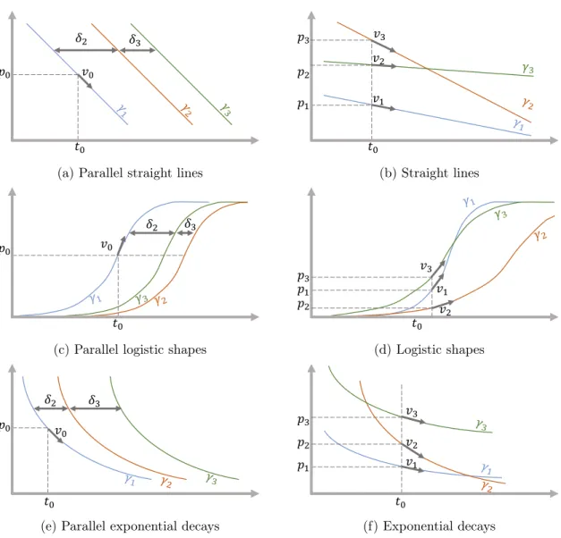
1.4 Different instantiations . . . 35
1.4.1 Parallel straight lines . . . 37
1.4.2 Straight lines . . . 37
1.4.3 Parallel logistic shapes . . . 37
1.4.4 Logistic shapes . . . 37
1.4.5 Parallel exponential decays . . . 38
1.4.6 Exponential decays . . . 38 1.4.7 Model variations . . . 38 1.4.8 Model selection . . . 39 2 Estimation 41 2.1 Statistical learning . . . 41 2.1.1 E-M algorithm . . . 42
2.1.2 Stochastic Approximization Expectation Maximization . . . 42
2.1.3 Monte Carlo Markov Chain SAEM . . . 43
2.1.4 Hasting Metropolis within Gibbs sampler . . . 44
2.2 Estimation of the disease progression model . . . 45
2.3 Calibration . . . 45
2.4 Personalization : estimate individual random effects . . . 46
2.5 Reconstruction, missing value imputation and future prediction . . . 47
Part II - Progression of Spatiotemporal Patterns for
Spa-tially Structured Data
493 Population and Individual Spatiotemporal Patterns of Progression from
Longitudinal Manifold-Valued Networks 51
3.1 Introduction . . . 52
3.2 Materials and Methods . . . 55
3.2.1 Sketch of the method . . . 55
3.2.2 Subjects and Data Preprocessing . . . 55
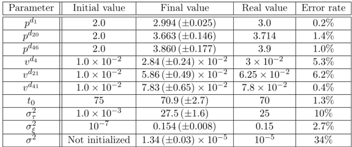
3.2.3 Model . . . 56 3.2.4 Algorithm . . . 60 3.2.5 Simulation study . . . 61 3.3 Results . . . 62 3.3.1 Initialization . . . 62 3.3.2 Population level . . . 65 3.3.3 Individual reconstruction . . . 65 3.4 Discussion . . . 68
4 Deciphering the Progression of PET Alterations using Surface-Based Spatiotemporal Modeling 71 4.1 Introduction . . . 71
4.2 Methods . . . 71
4.3 Results . . . 72
4.4 Conclusion . . . 73
Part III - Digital Multimodal Model of the Alzheimer’s
Disease Progression
75 5 Personalized Simulations of Alzheimer’s Disease Progression with Digital Brain Models 77 5.1 Introduction . . . 785.2 A geometric approach of statistical learning . . . 79
5.3 A multimodal disease progression model . . . 83
5.4 Reconstruction errors and generalisation to unseen data . . . 85
5.5 Personalized simulations of disease progression . . . 92
5.6 A holistic and dynamic view of disease progression . . . 96
5.7 Conclusion . . . 100
5.8 Methods . . . 101
5.8.1 Data Set . . . 101
5.8.2 Pre-processing and feature extraction . . . 102
5.8.3 Data representation and choice of Riemannian metrics . . . 103
5.8.4 Calibration . . . 105 5.8.5 Personalisation . . . 106 5.8.6 Prediction . . . 108 5.8.7 Conditional correlation . . . 108 5.8.8 Cofactor analysis . . . 108 5.8.9 Code availability . . . 109
Part IV - Simulation of Virtual Trajectories of
Progres-sion and Longitudinal Data Sets
1116 Simulation of Virtual Patients 113
6.1 Introduction . . . 114
6.2 Related Work . . . 116
6.2.1 Missing Values Imputation . . . 116
6.2.2 Data Augmentation Techniques . . . 116
6.3 Longitudinal Data Augmentation Framework . . . 117
6.3.1 Virtual Cohort Simulation . . . 117
6.3.2 Missing Values Imputation and Future Time-Points Prediction . . . 118
6.3.3 Improved Algorithms . . . 119
6.4 Longitudinal Model instantiation . . . 120
6.4.1 Statistical Model . . . 120
6.4.2 Estimation Procedures . . . 121
6.5 Experiments and Results . . . 122
6.5.1 Data Description . . . 122
6.5.2 Virtual Cohort Validation . . . 122
6.5.3 Missing Values Imputation . . . 123
6.5.4 Improved Prediction of Cognitive Scores . . . 125
6.6 Conclusion . . . 126
6.7 Supplemental materials . . . 128
6.7.1 Influence of hyperparameters on the simulation . . . 128
Part V - Software development
129 7 Estimation of the Disease Progression Model 131 7.1 Leasp : A C++ Software Package for the Analysis of Spatially Structured Longitudinal Data . . . 1317.1.1 Description . . . 131
7.1.2 Design . . . 132
7.1.3 How to use Leasp . . . 132
7.1.4 Support . . . 133
7.2 Leaspy : A Python Toolbox to Learn Spatiotemporal Patterns of Disease Progression . . . 134
7.2.1 Introduction . . . 134
7.2.2 Supported Classes of Problems & Related API functions . . . 134
7.2.3 Architecture & Software Design Principles . . . 136
7.2.4 Development . . . 136
8 Enhancement of Clinical Studies with Digital Tools 139 8.1 Introduction . . . 139
8.2 Applications . . . 140
8.2.1 General Requirements . . . 140
8.2.2 Long-term Disease Progression: www.digital-brain.org . . . 140
8.2.3 ADNI 1 Million . . . 142
8.2.4 Patient care with future prediction . . . 142
8.2.5 Dashboard for clinical studies . . . 143
8.3 Conclusion . . . 145
Valorization 151
Conclusion and perspectives 153
Appendix 1 169
8.4 Preambule . . . 169
8.4.1 Geodesic hypothesis . . . 169
8.4.2 Reparametrization and Likelihood . . . 170
8.4.3 Sufficient Statistics and Parameter Updates . . . 170
8.5 Parallel logistic shapes . . . 171
8.5.1 Geodesic hypothesis . . . 171
8.5.2 Reparametrization and Log-likelihood . . . 171
8.5.3 Sufficient Statistics and Parameter Updates . . . 172
8.6 Logistic shapes . . . 174
8.6.1 Geodesic hypothesis . . . 174
8.6.2 Reparametrization and Log-likelihood . . . 174
8.6.3 Sufficient Statistics and Parameters Update . . . 175
8.7 Exponential decays . . . 177
8.7.1 Geodesic hypothesis . . . 177
8.7.2 Reparametrization and Log-likelihood . . . 177
Résumé en Français
Motivation
La progression des maladies neurodégénératives dépend de phénomènes biologiques com-plexes qui restent mal compris, d’autant qu’ils se mettent en place sur des périodes de temps longues. De ce fait, décrire un scénario typique de l’évolution de la maladie est un enjeu majeur puisqu’il permettrait de mettre en lumière les dynamiques temporelles de différents biomarqueurs comme les tests neuropsychologiques, l’imagerie médicale ou les mesures physiologiques. Cependant, la description d’un scénario moyen de progression est confrontée à l’expression variable de la maladie à travers les patients, variabilité qui se traduit, par exemple, par des âges de diagnostics, des vitesses d’évolutions, des séquences et intensités d’événements divers.
Au vu de ces éléments, cette thèse s’emploie à d’écrire l’évolution typique de la mal-adie à l’échelle de la population, ce qui nécessite une caractérisation fine de la dynamique temporelle de différentes modalités. Au dela de cette description moyenne, le travail en-trepris tend à décrire la progression de la maladie à l’échelle individuelle, afin de (i) la comparer à l’évolution typique, (ii) prédire l’évolution future et (iii) analyser les cofacteurs à l’origine de cette variabilité, comme le sexe, les mutations génétiques ou des facteurs environnementaux. Ces analyses ne sont rendues possibles que grâce à une définition claire de la variabilité spatiotemporelle de l’évolution de la maladie.
Néanmoins, la progression des maladies neurodégénératives comprennent des spéci-ficités qui en rendent la description plus complexe que d’autres processus temporels. D’abord, bien que décrivrant un processus similaire chez tous les patients, son expression présente des caractéristiques individuelles propres, notamment l’absence d’alignement temporel en-tre les patients. Par exemple, la vitesse de progression de la maladie et l’âge au diagnos-tic sont suceptibles de différer d’un individu à l’autre. Typiquement, deux personnes du même âge peuvent présenter des stades d’avancement différents. A l’inverse, le même stade d’avancement peut apparaître à des âges différents selon les patients. Pour ces raisons, l’âge réel n’est pas un indicateur précis d’un âge physiologique qui correspondrait au stade de la maladie. Et déterminer ce dernier n’est pas aisé puisqu’il présuppose de désenchevêtrer l’impact de la maladie des caractéristiques naturelles des patients : les capacités cognitives, qui varient naturellement d’un individu à l’autre, en sont une illustration concrète. Ainsi, il est nécessaire de comparer correctement les évolutions individuelles les unes aux autres, et, potentiellement, à un scenario de référence. Malheureusement, définir ce scenario normatif est un défi puisqu’il demande de reconstruire une trajectoire sur des périodes de temps longues - plus longues que n’importe quelles mesures individuelles.
Toutes ces caractéristiques sont partagées par une majorité des maladies neurodégénéra-tives. La maladie d’Alzheimer nous livre l’exemple d’une telle dynamique temporelle, où les interactions entre la structure et les fonctions sont loin d’être parfaitement comprises, tout autant que leurs impacts sur les fonctions cognitives. Les phases précoces de la maladie sont caractérisées par des dépôts de plaques de protéines dans le cerveau, suivies par une modification de sa structure, conséquence d’une importante mort neuronale qui présente elle-même une dynamique propre. Les symptômes cliniques n’apparaissent que quelques années après, causant un dépistage de la maladie à des phases tardives où les fonctions et la structure du cerveau ont été modifiées de manière irréversible. De fait, il est devenu critique de déterminer les marqueurs précoces de la maladie.
Dans ce contexte, de nombreux modèles statistiques ont été développés pour ren-dre compte de l’évolution de différents biomarqueurs au cours de la progression de la maladie, à l’échelle de la population d’abord, puis des individus. L’un d’eux, introduit
dans [Schiratti et al., 2015], a permis de caractériser l’évolution moyenne de biomarqueurs scalaires au sein d’une cohorte, tout en interprétant chaque trajectoire individuelle comme la modification de l’évolution moyenne grâce à un nombre réduit de paramètres. La présente thèse étend le domaine d’application de ce modèle en introduisant des modèles de progression plus complexes, notamment pour des données d’imagerie médicale. D’autre part, la thèse présente des procédures mathématiques nécessaires à l’estimation des trajec-toires individuelles, rendant possible l’imputation de données manquantes et la prédiction de variables dans le futur. Enfin, le modèle est utilisé pour générer des données longitu-dinales virtuelles pour lesquelles on montre qu’elles peuvent se substituer à des données réelles, et, être utilisées par des prédicteurs qui requièrent d’importants volumes de don-nées.
Ces différentes contributions sont évaluées sur la capacité du modèle à décrire l’évolution de la maladie d’Alzheimer pour des scores cognitifs, l’épaisseur corticale, l’hypométabolisme et le maillage des hippocampes gauche et droit. A cette évolution typique s’ajoute l’analyse des cofacteurs (sexe, facteurs environnementaux, mutations génétiques) qui modifient cette évolution. Aussi, ce travail s’attache sur la capacité du modèle à prédire l’évolution future de patients atteints de troubles cognitifs précoces qui, dans certains cas, aboutissent à la maladie d’Alzheimer.
L’ensemble des modèles et algorithmes introduits dans cette thèse ont été regroupées dans le package Python Leaspy, permettant de conduire des analyses similaires sur d’autres cohortes, modalités et maladies neurodégénératives.
Présentation des parties
La Partie I est une introduction au modèle spatiotemporel de progression des maladies neu-rodégénératives. Ce modèle présente la volonté, d’abord, de décrire l’évolution moyenne d’une population, puis, d’estimer la variabilité spatiotemporelle de cette évolution dans la cohorte, et, enfin, de retracer l’histoire individuelle de la maladie à n’importe quel âge, de manière à imputer des données manquantes et prédire des valeurs futures. Le début de cette Partie s’attarde sur les notions fondamentales de géométrie riemannienne et d’estimations statistiques pour les modèles bayésiens à effets-mixtes, nécessaires à la compréhension générale du modèle. Ces notions permettent de construire un modèle spatio-temporel générique de progression des maladies neurodégénératives. S’ensuivent les instantiations de ce modèle pour la description de la progression de biomarqueurs qui présentent des pro-fils temporels linéaires, logistiques ou exponentiels. A la suite de la description géométrique du modèle, la seconde partie pourvoie le lecteur des outils indispensables aux procédures mathématiques suivantes : la calibration du modèle, la personnalisation aux données d’un nouveau patient, et, la simulation de données virtuelles - ou synthétiques. La calibra-tion permet d’estimer entièrement l’évolucalibra-tion typique de la maladie sur des périodes de temps longues. Elle repose sur l’algorithme Monte Carlo Markov Chain Stochastic Approx-imation Expectation Maximization, une version stochastique de l’algorithme Expectation-Maximization, où l’échantillonage des variables latentes est réalisé à l’aide d’une méthode de Monte Carlo par chaînes de Markov. La personnalisation, quant à elle, correspond à l’estimation des paramètres individuels qui décrivent l’évolution des variables d’un sujet. Cette étape rend possible l’imputation de données manquantes et la prédiction des vari-ables dans le futur. Enfin, la simulation est un moyen de synthétiser des patients virtuels qui reproduisent les caractéristiques des patients de la cohorte réelle. Ces patients virtuels peuvent être échantillonés sur une période de temps et avec un interval entre visites arbi-traires.
Tandis que la Partie I s’attarde à décrire la progression de variables scalaires, la Partie II s’intéresse à l’extension du précédent modèle pour des données qui présentent une structure
spatiale, au sens où certaines variables correspondent à l’évolution d’un même biomarqueur en des régions proches du cerveau. Cette structure se retrouve dans les images où les pixels voisins présentent a priori des caractéritiques similaires, mais également dans les atlas, les maillages, ... et toute donnée qui peut être représentée par un graphe dont chaque noeud intègre la progression au cours du temps de la valeur étudiée. Ce modèle est utilisé pour estimer l’évolution de l’épaisseur corticale au cours du temps, pour des patients qui développent la maladie d’Alzheimer. Dans un second temps, ce modèle est appliqué à l’estimation de la progression de traceurs radioactifs issus de PET scans, projetés sur la surface corticale.
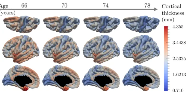
La Partie III est une étude approfondie du développement de la maladie d’Alzheimer, depuis les stades précoces jusqu’aux phases avancées. Elle reprend les modèles et algo-rithmes introduits dans les parties précédentes afin de les appliquer à différents types de données. De l’imagerie par résonnance magnétique (IRM), on extrait le maillage des hip-pocampes gauche et droit, et, l’épaisseur corticale en près de 3500 régions uniformément distribués sur la surface du cerveau. Aux IRM s’ajoutent les PET scans dont le rôle est de décrire l’évolution de la consommation de glucose dans le cerveau, projeté sur 120 régions du cerveau. Enfin sont ajoutés cinq scores cognitifs dont l’évolution est une manifestation de la maladie : perte de mémoire, des capacités de concentration, puis de la praxis et du language. Dans cette étude, il est montré l’évolution conjointe de ces modalités, illustrée sur le site www.digital-brain.org, ainsi que des cofacteurs (sexe, facteurs génétiques et environnementaux) qui modulent cette évolution. Enfin, une estimation des trajectoires individuelles permet de montrer l’intérêt de ce modèle pour, d’une part, reconstruire les données au niveau du bruit de mesure, et d’autre, part, de prédire leurs valeurs (scores cognitifs, volume de l’hippocampe et épaisseur corticale) jusqu’à quatre ans en avance.
La Partie IV tire profit de la capacité du modèle à décrire les évolutions individuelles des sujets en évaluant la variabilité spatiotemporelle de la progression. Il est alors possi-ble d’imputer des données manquantes et de prédire l’avancement de la maladie. D’autre part, le caractère génératif du modèle permet de simuler des patients virtuels à des stades différents de la maladie, avec un nombre de visite quelconque, et un échantillonnage tem-porel arbitraire. La qualité de ces patients virtuels est confirmée par l’impossibilité, pour un réseau de neurones adversarial, de distinguer des données réelles de données simulées. Enfin, ces dernières sont utilisées pour renforcer le pouvoir prédictif de réseaux de neurones récurrents, amélioraant la prédiction de certains scores cognitifs 3 et 4 ans à l’avance.
La Partie V reflète l’ensemble des développement logiciels produits au cours de la thèse. Ceux-ci incluent le package Python Leaspy qui permet d’utiliser les modèles et al-gorithmes précédents dans le cadre d’autres cohortes, modalités et maladies neurodégénéra-tives. Ce package a pour vocation de simplifier l’analyse de données longitudinales dans la recherche médicale, mais également d’être suffisament souple et structuré pour permettre l’implémentation de nouveaux modèles de progression et d’algorithmes d’estimation. En plus de cette librairie, ce sont des outils de visualisation et d’aide à la décision qui sont développés. On citera, parmi eux, des développements sur navigateur qui permettent, à partir de données individuelles, d’établir l’évolution future du patient pour un radiologue ou un neurologue.
Introduction
Motivation
Numerous phenomenon, such as people settlements, virus spreading or climatic evolu-tions, are governed by temporal interplays that make their description and comprehension challenging for the scientific community. Among them, the progression of neurodegener-ative diseases remains poorly understood due to complex interactions between multiple biomarkers that evolve through long periods of time. The description of a generic scenario of change is further hampered by the diversity and variability of individual evolutions in term of onset, pace, intensity and sequence of events. This consequently prevents from an accurate characterization of the individual disease progression. For these reasons, to over-come the lack of knowledge during the progression of neurodegenerative diseases, there has been a large interest over the past decades to model the disease progression, and its conse-quences on different modalities (e.g. cognitive assessments, medical imaging, physiological measurements), at both a population and individual level.
Arising in this historical context, the thesis aims at properly describing the typical his-tory of long-term disease progression which inevitably implies to characterize the complex temporal dynamics of inter-dependant modalities. On top of this average description, the work aspires to personalize this representative scenario of change to individual progressions in order to compare them to the mean, to study the influence of cofactors (e.g. gender, genetic mutations, environmental factors) and to enable a proper prediction of current and future time-points. Such a personalization pushes towards the definition and estimation of the spatiotemporal variability of disease progression within a population. All these el-ements pave the way to a sharper and more exhaustive analysis of the consequences of disease progression on diverse modalities.
Nevertheless, describing the progression of neurodegenerative diseases faces some par-ticular specificities compared to other temporal processes. First, even though it is, by def-inition, the evolution of an analogous phenomenon across patients, its expression present subject-specific patterns and characteristics. This is particularly highlighted by the tem-poral unalignment between individuals. For instance, the pace of progression or the age at disease onset might vary across patients. Typically, two persons sharing the same age might present a different disease stage. Said differently, the same disease stage is likely to appear at a wide range of ages. For that reason, the disease stage, as the expression of a physiological age along the disease development, better characterizes the disease and its progression than the observed age. However, the determination of this disease stage is restricted by the entanglement of the disease consequences with the natural character-istics of the patient. A typical example is the cognitive abilities that, despite declining during normal ageing or during the course of some diseases, are different within a popula-tion. This advocates for an unbiased comparison between individuals in order to determine properly the impact of the disease. However, the patients are observed during periods of time shorter than the long-lasting overall phenomenon - the latter never being observed fully and directly. This makes the comparison unlikely as there is no overall reference of a typical scenario of disease progression to compare to. Moreover, the very definition of a patient-wise disease stage is unclear as many evidence show that the temporal dynamics of the different biomarkers are not entirely related. This is revealed by the fact that the ordering of the (biological and clinical) events during the course of a disease, as well as their intensities, differ from one patient to another. Due to this variability, considering the existence of an overall disease stage involves that the later is characterized by potentially very different biomarker stages. Such a representation might be misleading and counter-productive as it associates into the same disease stage patients that have diverse biological
and clinical symptoms, preventing from an appropriate description of the disease. There-fore, it might be more accurate to refer to a disease status per biomarker, with complex interplays between the modalities, that finally result in a clinical stage.
All the aforementioned challenges characterize the progression of most of the neurode-generative diseases. An example of such heterogeneous dynamics is the Alzheimer’s disease where the specific role of the structure and of the functions of brain, as well as their in-teractions, on the cognitive decline remain unclear. First biological symptoms appear during the early, or prodromal, phase of the disease, such as the deposition of proteins plaques in the brain. They are essentially followed by a modification of the brain structure which is most of the time associated to a neuronal loss and consequently a diminution the brain metabolism. After a substantial amount of time (e.g. some years), they translate to clinical symptoms such as cognitive complaints and memory loss to finally end by an important dependence on relatives and medical staff. One of the obstacles to properly cure this decline is the fact that the clinical symptoms, i.e. the one that cause the medical examination and diagnosis, appear at late disease stages, when the neuronal loss is unduly important with no possible reversibility. Therefore, the importance to uncover, describe and analyze biomarkers during the course of a disease, especially those associated to early disease stage is crucial. This essentially means to properly understand both the temporal dynamic of each biomarker and their interactions. Such investigation might be undertaken at a population level by characterizing the long-term disease progression, but also at an individual level by identifying patients that will develop the disease at future stages. Some argue that such prediction is worthless as there is no potential treatment. We highlight here that this is actually a chicken-egg dilemma, the lack of treatment being the conse-quence of unsatisfactory disease modelings and predictions: describing the patients at risk enables to determine the critical biomarkers, common to these subjects, that result in a disease development. Moreover, one of the reason of lacking treatments is partly due to the fact that these treatment should be administered prior to the neuronal loss, at early stages of the disease i.e. in patients whose future prediction indicate a risk of disease development. Furthermore, the treatments may not be adequate for everyone but need to target subgroups of patients with similar patterns of progression. It again supports the idea that the disease should be adequately described and predicted at the different levels (e.g. structural, functional and cognitive) and to study how different cofactors modulate the biomarker progressions.
Therefore, investigating and exhibiting the biomarkers that are related to the disease progression pushes towards the development of appropriate tools that characterize the nat-ural long-term history of the disease. Such a description is made possible only if there is a adequate correspondence between a patient observation and its physiological age along the disease timeline. Recent developments in the medical field have raised promising results in predicting current status based on various measurements. Among many examples, we can cite the detection of breast cancer metastases [Bejnordi et al., 2017], the detection of a particular form of diabetes from retinal photographs [Gulshan et al., 2016], the predic-tion of cardiovascular risk from the same retinal photographs [Poplin et al., 2018] or the detection of cancer cells in lungs [Zhou et al., 2002]. All these impressive performances allowed to better identify the processes at stake during the related diseases. Though, they are predominantly - if not only - achieved for tasks that present multiple common charac-teristics: a clear definition of the problem, well-defined labels, significant knowledge about the underlying disease, ... In a word, tasks that are well-identified and rigorously described by the medical community and whose context is clearly set.
Unfortunately, these common denominators are not present in the case of neurodegen-erative diseases. In other terms, improving straightforwardly the accuracy of the disease stage prediction is an illusion when the disease is poorly understood. A typical example of such deficiency, in Alzheimer’s disease, is the limited number of labels associated to a
disease evolution that is continuous: the patients are either cognitively normal (CN), pre-senting mild cognitive impairments (MCI) or having Alzheimer’s disease (AD). The MCI stage corresponds to the premises of a dementia that can - or cannot - convert to AD: while the converters to AD are called progressive MCI, it is difficult to know whether the non con-verters, also called stable MCI, are intrinsically not developing AD (potentially in favor of another dementia) or because they pass away before an hypothetical conversion. Besides the lack of label granularity, the very own definition of Alzheimer’s disease has evolved during the last decades to describe realities that depend on the community. For some, it corresponds to clinical symptoms. For others, this past definition was based on symptoms that might be the result of different diseases or at least different patterns of progression that cannot be tackled simultaneously. They accordingly added biological characterizations to the disease. Nowadays, there is a tendency to distinguish Alzheimer’s pathology, i.e. a set of defined biological biomarkers, from Alzheimer’s disease, namely clinical symptoms. This reveals the ineffectiveness to predict a label, namely a disease stage, whose definition has not been properly set nor represents a homogeneous set of characteristics. Eventually, this is worsen by the trade-off between performance and interpretability, the former being predominantly chosen by the Machine Learning community. This is helpful in cases where the problems are well-defined but their determinants are too complex to be fully controlled and established by hand (by a doctor for instance). However, problems that are poorly defined and ill-posed are not susceptible to be improved in a substantial manner. This might be a reason of the somehow constant accuracy in disease progression over the past years. This is an additional reason to believe that explanability of the methods is key for disease that lack knowledge about their causes, effects and consequences.
For all these reasons, there is an intensive need to model and better understand the disease progression through its repercussions on different biomarkers and modalities. This necessarily involves to properly define and estimate the variability of individual progressions within a population. To this end, these complex dynamics should be accordingly inspected, described and analysed at both population and individual levels while considering the interplay of the different biomarkers.
Disease Modeling
To overcome the lack of knowledge about the progression of neurodegenerative diseases, there has been a large interest in disease modeling over the past decades. The first models have mainly been introduced by the medical community that has synthesized years of practical knowledge into so called hypothetical models as they are not directly supported by data evidence but rather field work and experience. In the case of Alzheimer’s disease, one of the most famous model was described in [Jack Jr et al., 2010b], shown on Fig. 1a. It was intended to present a hypothesis for the sequence of events that leads to Alzheimer’s disease. They hypothesized that there exists a cascade of consequential events that starts many years before the clinical symptoms, during the prodromal phase, that is characterized by protein plaques in the brain followed by a neuronal loss. They simultaneously highlighted the multi-modal aspects of the disease progression.
While they remain good starting points, these models remain hypothetical. And even though the first mathematical frameworks to order sequence of events have been intro-duced almost three decades ago [Beckett, 1993], they have not received much attention by the medical community because of the lack of large cohorts that were supposed to confirm or infirm the assumptions of the hypothetical models. These databases, essentially cross-sectional at the beginning, i.e. one observation per patient, contributed to the development of data-driven models that produced models of disease progression based on data evidence. Among them, [Fonteijn et al., 2012b] introduced the event-based model to characterize the sequence of events during the progression of Alzheimer’s disease and Huntington’s disease. Latter improved in [Young et al., 2014, Venkatraghavan et al., 2019], it essentially orders the observations to produce a sequence of events that occur during the disease progres-sion, as shown on Fig. 1b. This cascade does not measure the temporal evolution of each biomarker, nor the time delay between the apparition of two symptoms. Also, the vari-ability between individuals was only defined as an uncertainty in the cascade of events, represented by blocks of biomarkers that might occurs either simultaneously or with inter-vertions for different patients. Studies as [Huang and Alexander, 2012] defined an explicit variability of the model within a given population. This absence of temporal characteri-zation of the disease evolution was mainly due to the fact that age is a poor proxy of the disease stage. Among the attempts to circumvent this issue, [Iturria-Medina et al., 2016] considered the stage of the Alzheimer’s disease (CN, early MCI, late MCI and AD) as a proxy of the evolution to show the role of vascular disregulation during the course of the disease.
To overcome the issue of the temporal variability in the dynamic of disease pro-gression, longitudinal databases, namely multiple visits of patients, have been gathered. Hundreds of patients were followed during many years to measure various biomarkers (e.g. cognitive assessments or medical imaging) along with abundant cofactors (e.g. gen-der, genetics, socio-demographic attributes, comorbidities). While undoubtedly infor-mative, these databases bring together patients at different disease stages, with poten-tially different disease onset and pace of progression. To address this temporal vari-ability, [Jedynak et al., 2012] introduced an affine time-reparametrization of the real age t7→ αit+ βi onto the physiological age, considering that each subject presents a temporal
onset, or shift, βias well as an acceleration factor αi. The model was later extended to spa-tial data (e.g. PET amyloid imaging) that were converted into a disease score that allowed to realigned the observation while showing spatial correlation in the pattern of progression [Bilgel et al., 2015, Bilgel et al., 2016]. At the same time, [Donohue et al., 2014] consid-ered that each individual short-term measurements represent snapshots of the overall dis-ease progression. Once reparametrized, the patients observations can retrace the long-term evolution of the different biomarkers, as shown on Fig. 1d. Similarly, [Guerrero et al., 2016] described the individual trajectories as deviation of the group-average scenario of change.
(a) Hypothetical model of the cascade of events during the
disease progression. Courtesy of [Jack Jr et al., 2010b]. (b) Event-based model that rank the
sequence of events. Courtesy of
[Fonteijn et al., 2012b].
(c) Temporal realignment using the diagnosis as
proxy of the disease progression. Courtesy of
[Iturria-Medina et al., 2016].
(d) Temporal realignment of the individual ob-servations to reconstruct the group-average tra-jectory. Courtesy of [Donohue et al., 2014].
(e) Temporal realignment of the subject
measure-ments based on their spatial coherence. Courtesy of
[Marinescu et al., 2017].
(f) Derivation of the group-average trajectory to predict individual
fu-ture measurements. Courtesy of
[Iddi et al., 2019].
Figure 1: Evolution of the disease modeling in the last decades, from hypothetical broad models to individual specific prediction.
Such description corresponds to mixed-effects model, where the individual derivations take the form of random effects around the fixed effects that are shared by the population.
Recently, a probabilistic setting of evolution was introduced in [Lorenzi et al., 2017]. It also allows to realign the individual measurements along the disease axis. The follow-up measurements show to be very informative in the evolution modeling. However, it lacks a natural way to represent the variability in term of spatiotemporal progression. Another recent technique was introduced in [Oxtoby et al., 2018]. The authors relate the biomarker rate of change to the biomarker value itself, exploiting differential equations to model the disease progression.
The previous model essentially examined cognitive assessments or features derived from medical imaging, such as values of the cortical thickness or of the hypometabolism in spe-cific regions of interest, the volume of sub-cortical structures, the concentration of proteins in blood tests, ... Such studies, that go beyond univariate measures to analyse different modalities, essentially extract biomarkers prior to analyse their evolution. This is particu-larly true for imaged-based features. On the contrary, few studies explore the complexity of entire images. Among them, [Marinescu et al., 2017] recombine biomarkers from medical imaging measurements, taking advantage of the spatial structure of the disease progression. This allows to re-position the observations along the disease axis while aiming at clustering regions that are most likely to have a strong evolution during the disease history.
While most of the aforementioned models are able to define a group-average trajectory based on individual measurements, there are not suited to characterize individual progres-sions. Apart from the mixed-effects models, they do not provide a simple way to derive the long-term trajectory to individual observations. On the other hand, [Iddi et al., 2019] proposed a mixed-effects model used to predict future time-points, as shown on Fig. 1f, but whose overall explanability is made more complex due to the use of advanced Machine Learning algorithms. The authors of [Schiratti et al., 2015] introduced a generative mixed-effects model that similarly reconstructs the long-term disease progression from individual short-term measurements. Additionally, as the model considers the individual trajectories as spatiotemporal variations of the group-average one, it enables to derive estimation of the disease progression at an individual level. This is a first step to define continuous trajectories that define the evolution of the biomarkers at any time, potentially at fu-ture time-points. This description is made possible by the characterization of the overall spatiotemporal variability of evolution across subjects. The variability takes the form of random effects that, once estimated, define a probability distribution over the individual variables that modulate the typical scenario of progression. This distribution makes the model generative in the sense that it is possible to draw new samples. As each of them de-fines exactly the variations to the group-average scenario of progression, it entirely dede-fines a new patient that reproduce the characteristics of the real patients, while being simulated and thus anonymous.
To sum up, over the last decades, models that first described the general trend of the disease progression, slowly considered a time-realignment of the individuals to get the average sequence of events. Along the way, some proposed to convert this sequence to a temporal dynamic and ordering, including more complex modalities. Finally, recent advances helped to go from a group-average trajectory to a individual description of the disease progression. These improvements were associated to the increasing complexity of the biomarkers analyzed. Unfortunately, they did not necessarily investigate the multi-modal aspects of the disease, especially their separate but dependant temporal dynamics. This advocates for a general framework to study the changes of different biomarkers under the influence of the disease evolution.
The work detailed in this thesis follows this historical development, especially from the work initiated in [Schiratti, 2016]. It tackles the challenges raised by the complex temporal dynamics of each biomarkers, which also present specificities at the individual level, to :
• describe the typical scenario of disease progression, from prodromal to clinical stages, • personalize this average trajectory to individual progressions, enabling an in-depth
study of the cofactors that modulate this progression,
• characterize the individual trajectories to impute missing values and predict future stages,
• properly estimate the variability of disease progression to simulate virtual cohorts of anonymized individuals.
While [Schiratti, 2016] introduced the spatiotemporal model to essentially address the first point, especially for scalar biomarkers, this manuscript aims at further investigating the three remaining challenges for a larger family of spatiotemporal models of progression and to include multiple modalities such as the thickening of the cortical structure, the brain glucose consumption as a marker of the hypometabolism, and the decline of the cognitive abilities. It inevitably involves to analyze data that have different characteristics such as their acquisition, their dimension and resolution, their measurement noise and or inter- and intra-individual variability. Therefore, this work, while analysing and comparing heterogeneous data, is built with the intention to be adaptable to different modalities and biomarkers.
Conceptual overview
To ease the reading and understanding of the proposed model, we first start by exem-plifying the problem at hand: the characterization of a temporal trajectory given some measurements. Let us describe the growth of a child given his pictures at different ages. We consider a fixed camera that shots a plain-size picture of a child at 6 and 12 months (on a white background), as shown on Fig.2. Each picture, represented by a blue dot, has N pixels, each being valued between 0 and 255, such that the feature space is ]0, 255[N.
The picture of the same person at 9 months old also belongs to this space but it is easily understandable that this picture is not the mean (in the Euclidean space) of the two pre-vious pictures: the mean, i.e. the mean of the pixels, results in the blurry version of the superposition of the first pictures, as shown on Fig. 2. On the other hand, the collection of all the pictures between 6 and 12 months defines a curve (in a sense to be precised) in the feature space, represented by the black curve, that corresponds to the individual trajectory. As we can theoretically define this trajectory for any individual, the set of all the resulting curves results in a subspace of the initial embedding space that we model by the blue-to-red surface on Fig. 2. This subspace, called a Riemannian manifold (see Chapter 1), allows to perform calculus between images, for instance to exhibit the picture at 18 months old by following the black curve on this manifold.
ℝ
𝑵Picture at
6 months Unseen picture Picture at 12 months
at 9 months
Hypothetical picture at 18 months
Euclidean mean of the 6 and 12 month old pictures
Figure 2: The pictures (blue dots in the space of measurements RN) belongs to a subspace, illustrated by the blue-to-red surface that corresponds to the space of possible pictures during the growing. This subspace circumvents the inability of the Euclidean mean to compute the mean picture between 6 and 12 months. It also enables to predict future pictures, for instance at 18 months, based on the trajectory (black curve) that is estimated from the first pictures.
While the mathematical formalism of this modeling is described in Chapter 1, same logic applies to the modeling of the individual spatiotemporal trajectories of disease pro-gression. In the case of longitudinal databases, the repeated observations of the subjects are represented by the colored dots on Fig. 3. The collection of all possible observations is represented by the blue-to-red surface. As in the previous example, the individual trajecto-ries are represented by curves on this surface. In the particular case of disease progression, while individuals are mostly observed during short-term periods, we make the hypothe-sis that there exists a long-term group-average spatiotemporal trajectory represented by
the black curve. The latter should be considered as the recombination of the individual snapshots, each providing consistent information about a particular disease stage. By con-struction, it consequently spans a longer time-window of disease progression. To account for the spatial variability, i.e. the fact that there is a distance between the group-average and individual curves, we consider that there exists a spatial shift from one to the other. On top of that, the temporal variability is modeled through a temporal reparametrization of the progression along the curves. It enables a time shift of the disease onset as well as an acceleration factor that modulates the individual speed of progression. To these spatiotemporal variability, we highlight that the subjects are observed at different stages, with different baseline ages and a different number of times. These characteristics, while being potentially difficult to handle, are actually key to provide necessary information to reconstruct the overall disease progression over a long period of time.
ℝ𝑵
Group average trajectory
Individual trajectory with 4 observed measurements
Figure 3: Given the space of possible observations represented by the blue-to-red surface, the dots are the measurements such that the colors indicate the patient they belong to. The corresponding curve is the individual trajectory that can be recombine into a long-term group-average trajectory in black. The trajectory present an important variability in term of number of measurements, distance to the mean curve, potentially the stage at the first visit.
Fig. 3 finally shows that this modeling allows to both characterize the group-average long-term trajectory while personalizing this progression to individual measurements. Be-yond the possibility to achieve the two aforementioned goals, this figure illustrates that this embedding provides a framework (detailed in the next chapters) that also enables to:
• accurately compare the individual spatiotemporal progressions thanks to their rela-tive positioning to the mean, in particular by studying the cofactors that significantly modulate the disease progression,
• reconstruct particular values along the individual trajectory to either impute missing values or predict future time-points by extrapolating the timeline,
• properly determine the space of possible measurements and trajectories to generate virtual individuals with longitudinal measurements that enables first to un-bias or balance initial cohorts and to enhance the predictive power of algorithms that require large amounts of data.
To demonstrate that this model provides an adequate framework to study the disease progression, at both an average and individual level, we concentrate our attention on the study of Alzheimer’s disease, especially the synchronized evolution of the cognitive func-tions, the hypometabolism and the structure of the brain. This first requires to consider a generic model suited for data that present different characteristics in term of structure or dimensions, e.g. vectors of cognitive assessments, positron emission tomography (PET) and magnetic resonnance imaging (MRI). Once formulated, the model is evaluated on its capacity to characterize the long-term disease progression and to reconstruct the individual trajectories. The quality of the latter is assessed by their comparison to the intrinsic noise in the data which is to be determined and measured (e.g. test-retest data, medical imaging resolution, feature extraction). As these reconstructions are made possible thanks to the estimation of a continuous individual trajectory, it further enables to impute missing values and predict the biomarkers at future time-points, up to 4 years in advance. Finally, the ability of the model to properly estimate the variability in term of disease progression en-ables the simulation of virtual patients with longitudinal measurements, that once gathered into a virtual cohort, can be shared without violating sharing policies as anonymization.
This framework can provide promising tools to the medical community to better un-derstand diseases and their underlying mechanisms. To this end, special attention has been given to the development of numerical tools that can be used efficiently by both the medical and research community. We dedicated the website www.digital-brain.org to an interactive digital model of the Alzheimer’s disease progression that can be modified to exhibit individual scenarios of evolution. Furthermore, the Leaspy Python package has been released to enable researchers to estimate similar disease progression on other biomarkers, modalities, cohorts and diseases.
Manuscript overview
The first part is a general introduction to the generative mixed-effects model presented in this thesis. It first exposes the mathematical definitions and tools needed to define the generic model of progression. It then presents particular instantiations of the model that suit different profiles of disease progression. Finally, it describes the mathematical operations that allow to reconstruct the group-average scenario of change, to personalize it to individual measurements, to impute missing values, to predict biomarkers at future time-points and, finally, to simulate virtual patients.
The second part introduces a model that is better suited to describe the disease progres-sion for data that present a spatial structure. It includes medical imaging and network-values measures. The model ensures a spatial coherence of the disease progression for neighbor regions. This is validated by characterizing the cortical atrophy and the brain metabolism decrease during the course of Alzheimer’s disease.
The third part extensively describes and validates the possibilities offered by this dis-ease progression framework. We consider a large scale longitudinal database of Alzheimer’s disease from which we use cognitive assessments and medical imaging derived data (cortical thickness over the entire brain, deformation of the hippocampus meshes and FDG-PET data) to reconstruct the long-term disease progression. This demonstrates the reconstruc-tion of the individual data up to the noise level and the predicreconstruc-tion of future time-points. It comes with a finer description of the disease mechanisms during the course of the disease
The fourth part takes the most out of the generative and mixed-effects characteristics of the model: it allows to simulate patient’s missing or future observations and also virtual patients. The simulated observations can either be used to impute missing values or to predict future timepoints. On the other hand, the simulation of virtual patient enables to un-bias or unbalance real cohorts for under-represented subgroups. In both cases, the resulting virtual cohort helps improving algorithm predictive power in order to reach state of the art results in the long-term prediction of cognitive impairments.
The fifth part describes the digital tools developed during the thesis. First, the Python package Leaspy allows to run similar analysis on new cohorts for potentially other (neu-rodegenerative) diseases. Then, we develop a digital model that relates for the long term progression of the disease for different modalities. Finally, we propose a clinical dashboard to monitor patients in a clinical study or in real life.
Part I
Spatiotemporal Model of Progression
from Longitudinal Data
Chapter 1
Scalar Models and Extensions
This chapter first briefly introduces the key mathematical concepts of the manuscript the model is build on, i.e. the Riemannian geometry and the mixed-effects models. It cannot be considered as a detailed or exhaustive description of these mathematical notions, but rather a glimpse of the tools that are essential to the understanding of the following chapters. However readers that are eager to understand the formal mathematical background of the corresponding topics are referred to the mentioned references. In a second part, the chapter introduces the generative mixed-effects model of disease progression. It starts with the mathematical description of the model, in its generic form, thanks to the Riemannian geometry setting. It then gives multiple instantiations of the model before discussing some of its properties.
Contents
1.1 Riemannian geometry . . . 30
1.1.1 Manifold . . . 30
1.1.2 Metrics and Riemannian manifolds . . . 30
1.1.3 Geodesics . . . 30
1.1.4 Exponential mapping . . . 31
1.1.5 Parallel-transport . . . 31
1.2 Mixed effects models . . . 31
1.2.1 Linear mixed effects models . . . 32
1.2.2 Non linear mixed effects models . . . 32
1.2.3 Longitudinal data in the case of biological phenomenon . . . 32
1.3 Disease progression model . . . 34
1.3.1 Geometric description . . . 34
1.3.2 Statistical description . . . 35
1.3.3 Identifiability conditions . . . 35
1.3.4 Product of 1D models . . . 35
1.4 Different instantiations . . . 35
1.4.1 Parallel straight lines . . . 37
1.4.2 Straight lines . . . 37
1.4.3 Parallel logistic shapes . . . 37
1.4.4 Logistic shapes . . . 37
1.4.5 Parallel exponential decays . . . 38
1.4.6 Exponential decays . . . 38
1.4.7 Model variations . . . 38
1.1
Riemannian geometry
In the introduction, we made the hypothesis that the data of interest belong to a particular subspace of the feature space, that individual trajectories are described by curves on this subspace and that the repeated observations are points on these curves. This subspace is thus central to the disease modeling as it entirely defines the space of possible measurements and consequently the individual spatiotemporal trajectories. To this end, we introduce the Riemannian geometry that is well suited to define such spaces but also to derive mathematical notions such as curves and distances on this space. Historically, it has been introduced to study differentiable topological spaces embedded in Rn. These spaces, called manifolds, are characterized by the associated metrics that allows to generalize the notion of distances in Euclidean spaces to such manifolds. We then introduce the concept of geodesics that characterizes curves in these non Euclidean spaces. Finally, we define the concept of parallel transport which is an important tool to shift (in a sense to be precise) the previous curve to other regions of the manifold. This theoretical framework is extensively presented in [Do Carmo Valero, 1992].
1.1.1 Manifold
A manifold is a topological space for which each point presents a neighborhood that is homeomorphic to the Euclidean space. Simply said, there exist a collection of mappings (called atlas) from regions of this space (as defined in [Do Carmo Valero, 1992]) to linear spaces. It is possible to make calculus on each of this linear space and to derive it to the corresponding region ; that leads to a locally differentiable structure. However, if these local differentiable structures are continuous (in some sense [Do Carmo Valero, 1992]) from one local mapping to the other, then the differentiable structure is said to be globally differentiable. This defines a differentiable manifold or smooth manifold.
Given a smooth manifold M of Rn, each point p ∈ M is associated to its tangent space TpM that is a linear approximation of the manifold in the neighborhood of p. This
tangent space contains all the possible derivations of M at p, intuitively corresponding to the vectors at p in the direction of the derivations. These derivations are made possible at each point of the smooth manifold by the differentiable structure.
1.1.2 Metrics and Riemannian manifolds
We consider a smooth manifold M such that each point p∈ M is associated to an inner product gpon the vector field of the tangent space TpM, which varies smoothly from point
to point. The collection gM= (gp)p∈Mis called a metric on the manifold. This generalizes
the Euclidean scalar product to manifolds. Equipped with this metric, (M, gM) is called
a Riemannian manifold. This key concept allows to introduce, among others, the notion of distances on this differentiable structure.
1.1.3 Geodesics
The geodesics are to Riemannian geometry what straight lines are to Euclidean spaces: they correspond to curves that to some extend represent the shortest path between two points of the underlying manifold. Formally, given a smooth curve γ : I ⊂ R → M, we say that γ is a geodesic of M if ∇γ˙˙γ = 0, i.e. a smooth curve with zero acceleration
(∇ corresponds to the Levi-Civita connection, see [Do Carmo Valero, 1992] for technical details).
Ri sk o f di se as e de ve lo pm en t Blood pressure 0 mutation 1 mutation 2 mutations
(a) Each point being the observation of a pa-tient, the risk of disease development depends on the blood pressure (fixed effect) and the number of mutations of a given allele (random effect). Vo lu m e of th e br ai n Age Observation of the same individual Average tra jectory
(b) Considering repeated observations per sub-ject, a standard linear regression (grey dashed line) returns unexpected results. A random-slope random intercept model is better suited to describe the individual variability.
Figure 1.1: Examples of mixed effects models in the case of (a) independent data and (b) longitudinal data with repeated observations per subjects. They are better suited than standard tools (e.g. standard linear regressions) to combine population and individual effects.
1.1.4 Exponential mapping
We consider a point p ∈ M, a velocity v ∈ TpM and a geodesic γ such that γ(t) = p and ˙γ(t) = v. It can be shown that such geodesic is unique so that we rewrite it γ := Expp,t(v) : t7→ Expp,t(v)(t). The exponential mapping associates the vector v to the point reached by this geodesic at time t+ 1. It writes v∈ Tp 7→ Expp(v) = Expp,t(v)(t + 1).
It is essentially a step on the manifold from p in the direction of v.
1.1.5 Parallel-transport
Given a manifold M and a smooth curve γ : I ⊂ R → M, a vector field X is said to be parallel along γ if DXdt = 0. Given w0 ∈ Tγ(t0)M, one can show there exists a unique
vector field w(t) parallel along γ such that w(t0) = w0. This corresponds to the transport
of w0 along γ such that the vector field w(t) remains parallel to w0. This notion is crucial
to compare calculus across tangent spaces along a geodesic.
1.2
Mixed effects models
While Riemannian geometry is fundamental to characterize the space of possible measure-ments, it does not provide a formulation of the individual nor the population trajectory of disease progression on these Riemannian manifolds. To this end, we introduce the mixed effects models [Fisher, 1919, Fisher, 1992]. They are statistical models which combine, in the description of a phenomenon, the contribution of global effects affecting all the obser-vations, and, the contribution of individual effects that are specific to each observation. On the one hand, the global effects are called the fixed effects: they are non-random quantities that best describe the whole population; one can think of the slope and the intercept as the fixed effects of a linear regression because they affect equivalently all the observations. On the other hand, the individual variability is described by random perturbations of the fixed-effects, called the random effects, that allow to derive the individual observations from the population-wide description. They essentially characterize the overall variability in the population. An example of such mixed-effects model is shown on Fig. 1.1a.