HAL Id: hal-00013378
https://hal.archives-ouvertes.fr/hal-00013378v2
Preprint submitted on 16 May 2006
HAL is a multi-disciplinary open access
archive for the deposit and dissemination of
sci-entific research documents, whether they are
pub-lished or not. The documents may come from
teaching and research institutions in France or
abroad, or from public or private research centers.
L’archive ouverte pluridisciplinaire HAL, est
destinée au dépôt et à la diffusion de documents
scientifiques de niveau recherche, publiés ou non,
émanant des établissements d’enseignement et de
recherche français ou étrangers, des laboratoires
publics ou privés.
Woodrow Shew, Sébastien Poncet, Jean-Francois Pinton
To cite this version:
Woodrow Shew, Sébastien Poncet, Jean-Francois Pinton. Force measurements on rising bubbles. 2006.
�hal-00013378v2�
Woodrow L. Shew, Sebastien Poncet, and Jean-Fran¸cois Pinton Laboratoire de Physique, ´Ecole Normale Sup´erieure de Lyon
Lyon, France 69007
The dynamics of millimeter sized air bubbles rising through still water are investigated using precise ultrasound velocity measurements combined with high speed video. From measurements of speed and three dimensional trajectories we deduce the forces on the bubble which give rise to planar zigzag and spiraling motion.
I. BACKGROUND
An understanding of bubble-fluid interactions is impor-tant in a broad range of natural, engineering, and med-ical settings. Air-sea gas transfer, bubble column reac-tors, oil/natural gas transport, boiling heat transfer, ship hydrodynamics, ink-jet printing and medical ultrasound imaging are just a few examples where the dynamics of bubbles play a role (e.g [6, 16, 26]).
We narrow our focus to a single air bubble rising through still water. The buoyant force which drives the bubble’s rise does work resulting in an increase in kinetic energy of the surrounding fluid. This induced flow, in turn, gives rise to hydrodynamic forces on the bubble and hence changes in the bubble trajectory. The mea-surement of these forces is the aim of the experimental work presented here
Our study includes a range of bubble sizes between 0.84 and 1.2 mm in radius. At the small end of this range the bubble’s path is rectilinear. As the bubble size is in-creased, one observes a transition to a planar zigzag path [8, 23]. A second instability, often preceded by the zigzag, results in a spiraling path [5, 8, 15, 23]. For even larger bubbles, a third type of oscillating path occurs, which has similarities to the zigzag, sometimes called “rock-ing”. We do not address this state and emphasize that it is different than the zigzag mentioned above. Unlike the zigzag state that we study, the rocking bubble un-dergoes dramatic shape oscillations and the frequency of path oscillation is several times higher than the zigzag or spiral [5, 15]. Our approach is to use well resolved measurements of three-dimensional bubble trajectories to calculate the hydrodynamic forces on the bubbles.
The dynamics of bubble path instabilities have puzzled researchers for quite a long time. Leonardo Da Vinci is likely the first scientist to have contributed to the signif-icant body of work addressing this problem [26]. Clift, Grace, and Weber [6] review relevant studies prior to about 1978. In 2000, Magnaudet and Eames [16] pro-vided a thorough account of more recent work on this subject. Our attention will be limited to those works which address path instabilities of bubbles less than 2.5 mm in diameter. Saffman [27], Hartunian and Sears [11], and later Benjamin [4] attempted to explain fea-tures of the path instabilities and bubble shape by an-alytical means, but experiments are not in accord with their findings.
Several experimental works have visualized and doc-umented zigzagging and spiraling bubble paths. Ay-bers and Tapucu [1, 2]used photographic techniques to measure bubble speed, drag coefficients, size, shape, and path. Mercier, Lyrio, and Forslund [17] used a strobo-scope and several cameras to measure short sections of bubble trajectories. More recently, Wu and Gharib used a high speed video three-dimensional imaging system to measure paths and bubble shape. These works advanced qualitative understanding of bubble behavior without at-tempting to explain causal mechanisms or make detailed quantitative force measurements.
Other recent studies have investigated path instabili-ties with special attention paid to the role of the bub-ble’s wake. Lunde and Perkins [15] used dye to ob-serve the wake of ascending bubbles and solid particles. Br¨ucker [5] used particle image velocimetry to study the wake of large spiraling and rocking bubbles. Mougin and Magnaudet [22, 23] presented numerical observations of the path and wake of a bubble with a rigid ellipsoidal shape. de Vries et al. [8] used Schlieren optics techniques to visualize the wakes of zigzagging and spiraling bub-bles. Finally, Ellingsen and Risso [10] used laser Doppler anenometry and cameras to measure the path as well as the flow around the bubble.
These studies have revealed a wake consisting of two long, thin, parallel vortices aligned with the bubble’s path. One vortex rotates clockwise and the other counter-clockwise. For a spiraling bubble the wake vor-tices are continuously generated, while they are inter-rupted twice per period of path oscillation for the zigzag. Mougin and Magnaudet [22, 23] observed a nearly identi-cal wake structure in their numeriidenti-cal simulations (see also [24]). It is believed that the wake vortices play a critical role in generating hydrodynamic forces on the bubble.
In the next section we describe the experimental appa-ratus and measurement techniques, as well a typical bub-ble trajectory. In section III, we present a method for ex-tracting force measurements from path and velocity mea-surements based on the generalized Kirchhoff equations. Then, in section IV, we discuss some observations of the bubble trajectory during the first few hundred millisec-onds after release. We describe observations and force measurements for zigzagging bubbles in section V and spiraling bubbles in section VI. Finally, our results are summarized in section VII.
ultrasound PC camera PC freq gen freq gen amplifier amplifier A/D mixer peristaltic pump stainless steel capillary bottom lighting camera ultrasound emitter ultrasound receiver top lighting top lighting 200 cm
FIG. 1: Schematic of experimental setup. As the bubble rises its vertical velocity is measured using ultrasound and its hor-izontal position is obtained with a high speed video camera.
II. EXPERIMENTAL APPARATUS AND
METHODS
One goal of this work is to obtain measurements of bubble behavior rising through a large distance, reveal-ing the long time dynamics of the zigzag and spiral in-stabilities. To this effect, the experiments are conducted in a tank 2 m in height and 30 cm wide with square cross section as illustrated in Fig. 1. The walls are made of 1.45 cm thick acrylic plate. Bubbles are produced at the bottom of the vessel by pumping air through a 24 gauge stainless steel capillary tube with a 0.30 mm inner di-ameter (ID) and a 0.56 mm outer didi-ameter (OD). The tube is oriented with its open end facing upwards. The air is pumped to the capillary tube through a length of Tygon tubing (0.51 mm ID and 2.3 mm OD, from Cole-Parmer) using a peristaltic pump (Roto-Consulta, flocon 1003). The rotor of the pump is turned by hand, releas-ing a sreleas-ingle bubble. We always allow at least 3 minutes delay between the release of consecutive bubbles to be sure that the water is truly quiescent for each bubble.
The volume of each bubble is measured individually. When the bubble reaches the top of the vessel it is
0.6 0.8 1 1.2 1.2 1.4 1.6 1.8 2 2.2 2.4 aspect ratio χ bubble radius (mm)
FIG. 2: Comparison of Duineveld’s [9] measurements of as-pect ratio and the linear model we use to estimate χ.
trapped under a submerged plate. Using a syringe, each bubble is sucked into a transparent section of Tygon tub-ing (ID 0.51 ± 0.005 mm) with water on either side of the bubble. The length of the air plug in the tube is then measured with calipers (± 0.2 mm precision). Knowing the tube inner diameter one then calculates the bubble volume. In the results that follow, an equivalent radius
R ≡ (3/4π×actual volume)1/3is used as a measure of the
bubble size. During the ascent, R increases by 6% due to the gradient in hydrostatic pressure. This expansion is accounted for in the calculations of forces. Furthermore, each instance where the bubble radius or Reynolds num-ber is presented in this paper it is properly adjusted for the pressure at the height of the bubble being described. The Reynolds number is defined Re = 2RU/ν, where
U is the current speed of the bubble and ν is the
kine-matic viscosity of water. We have observed speeds in the range 32 < U < 36 cm/s, yielding Reynolds numbers 500 < Re < 770.
Some of our force calculations depend on the shape of the bubble. It has been shown by other experimen-tal studies that the bubble is close to an oblate ellipsoid [7, 9, 10]. Since we do not make such measurements, we use the experimental results of Duineveld [9] to estimate the shape of our bubbles. Wu and Gharib [30] measured aspect ratios which confirm Duineveld’s results. The as-pect ratio of the bubbles in our size range is well approx-imated by a linear function of bubble equivalent radius. The aspect ratio χ is defined as the length of the semi-major axis divided by the length of the semiminor axis. In fig. 2, we show Duineveld’s results and the linear fit,
χ(R) = 2.18R − 0.10. (1)
This method of estimating χ is supported by the agree-ment of our measureagree-ments with Moore’s [18] drag theory as shown below in Fig. 7, section IV.
Before each experiment the vessel and all parts exposed to the water are thoroughly cleaned with methanol, dried, and then rinsed with tap water for 5 minutes. All data is collected with tap water less than 8 hours old. It is
known that small bubbles rise more slowly in tap water compared to highly purified water due to contamination of the air-water interface with surfactants (e.g. [6, 9]). Nonetheless, several observations suggest that surfactant effects are not greatly influencing the dynamics of our bubbles, probably because of their larger size. First, our velocity measurements are consistent with Moore’s drag theory and Duineveld’s measurements in clean water (see fig. 7 in section IV). Second, we observe that during the straight rise of a bubble of radius 1.0 mm (at 1 atm), the velocity grows by about 2% over 1.5 m. This result is consistent with the increase in buoyancy and drag due the expansion of size as well as aspect ratio during ascent. If surfactant effects were significant, the bubble would likely slow down as it rises. We note that for bubbles smaller than about 0.75 mm in radius, our measured rise velocities reveal such a decrease in speed and are lower than those reported by Duineveld. This indicates that, in our tap water, smaller bubbles are strongly influenced by surfactants, while larger bubbles are not. The data presented in this paper is limited to bubbles larger than 0.87 mm.
Temperature is monitored at two different depths for each experiment. The mean temperature is 18.5±0.25◦C
and the temperature gradient is always less than 0.009
◦C/cm.
The trajectory of the bubble is measured using two methods: ultrasound and high speed video. The vertical component of the bubble velocity is obtained with high precision using a continuous ultrasound technique. We briefly describe this technique here, but for more detail the reader is referred to [19–21]. One piezo-electric ul-trasound transducer positioned at the top of the vessel generates a continuous 2.8 MHz sound wave directed to-wards the bottom. The emitted waveform is created by a Agilent arbitrary function generator (E1445A) and am-plified by a Kalmus Engineering Model 150C 47 dB radio frequency power amp. The sound is scattered by the ris-ing bubble and measured by an array of eight piezo ultra-sound transducers (custom by Vermon), also located at the top of the vessel. Each signal measured by the eight receiving transducers is then mixed into a different fre-quency band, amplified, and summed using an in-house custom made circuit. After this stage, 130 dB of dynam-ical range is preserved. The eight channels are mixed down to one channel so that only one analog to digital converter is needed to digitize the data. The digitiza-tion is accomplished with a Agilent 10 MHz, 23 bit A/D converter (E1430A). All of the Agilent devices are VXI modules in a Agilent mainframe (E1421A) which inter-faces with a personal computer using a fire-wire module (E8491A).
Once digitized, Matlab routines are used to extract the original eight channels of ultrasound data. The signal from each channel is dominated by the emitted frequency (2.8 MHz) and a lower amplitude Doppler shifted fre-quency of the sound scattered from the bubble. Each sig-nal is shifted in frequency so that the emitted frequency
becomes DC and hence the Doppler shifted frequency is directly proportional to the bubble velocity. In order to obtain velocity as a function of time the frequency is ex-tracted using a numerical approximated maximum like-lihood scheme coupled with a generalized Kalman filter [19].
The ultrasound method measures the component of the bubble’s velocity along the line between the bubble and the ultrasound receiver. In order to obtain the true ver-tical component, some correction of the data is required as the bubble comes closer to the ultrasound transducer. An iterative corrective algorithm is employed beginning with the average vertical velocity and the position data from the camera data as a first estimate of the trajectory. Geometrical corrections are then made on the original ve-locity data based on this approximate trajectory. This new corrected velocity is then used to recompute the tra-jectory. The process is then iterated until convergence is reached.
The absolute accuracy of our velocity measurements was verified using a video camera. We released an object slightly heavier than water and recorded its steady de-scent with the ultrasound device and simultaneously with a camera positioned 2.5 meters away with a side view of the tank. The test showed that the ultrasound velocity measurements are consistent within 2% of the camera data. We measure top speeds of our bubbles typically about 36 cm/s, which is consistent with other experi-mental measurements [2, 9, 30]. The relative accuracy of our velocity measurements is more precise, typically
±1 mm/s, or about 0.2% accuracy. Furthermore, the
sampling frequency is several kHz. Over a distance of 2 meters, this level of accuracy is not possible with cam-eras or other optical methods. Another advantage is that the ultrasound technique is potentially useful in opaque fluids.
The vertical velocity measurements provide direct ob-servations of the kinetic energy delivered to the fluid as the bubble rises. The only energy source in the system is the work done by the buoyancy force Fb. The power
delivered to the fluid is then Fb · U = ρV gUz, where
ρ = ρf − ρg is the density difference between the fluid
and the gas, V is the volume of the bubble, g is acceler-ation due to gravity, and Uzis the vertical component of
velocity of the bubble. Note that ρg¿ ρf, so ρ ≈ ρf. In
the remainder of this paper we will continue to neglect the density of the gas. For typical bubbles in our study,
Uz≈ 0.35 m/s and the buoyancy force is ρV g ≈ 50 µN.
Therefore the bubble produces about 10 µW of power in the form of fluid kinetic energy as it rises.
A high speed video camera (Photron Fast Cam Ultima 1024) is used to obtain the horizontal motion of the bub-ble. The camera is positioned above the vessel close to the ultrasound receiving array so that it records the lat-eral movement of the bubble. The camera is operated at 125 frames/sec with 512 × 512 pixel resolution. The bubble is between 10 and 100 pixels wide as it rises from a depth of two meters. Lighting is provided by two
in-candescent lamps (125 and 100 Watts) positioned above the vessel and one (100 Watts) beneath the translucent floor. Note that most of the time series displayed later in this paper contain 125 samples/sec since they are at least partially derived from the camera data. This gives an effective time resolution of 8 ms. Time series with higher sampling rates (see section IV) are derived only from the ultrasound data, which yields a time resolution of less than 1 ms. The period of motion for typical path oscillations is around 200 ms.
The bubble position is extracted from movies using another Matlab routine. The routine subtracts frame i from frame i + 1, then averages over a 5 × 5 pixel moving window and locates the maximum of the resulting image. This process is repeated, reversing the subtraction (frame
i minus frame i + 1). The position of the maxima of the
two subtraction/averageing processes are then averaged and taken as the bubble position. This method is found to reliably locate the bubble center even when the camera focus and light reflected from the bubble changes during its ascent. The accuracy of the position measurements is about 3% or ± 0.1 mm. The horizontal position data is differentiated to obtain the horizontal velocity with about 6% or ±6 mm/s precision.
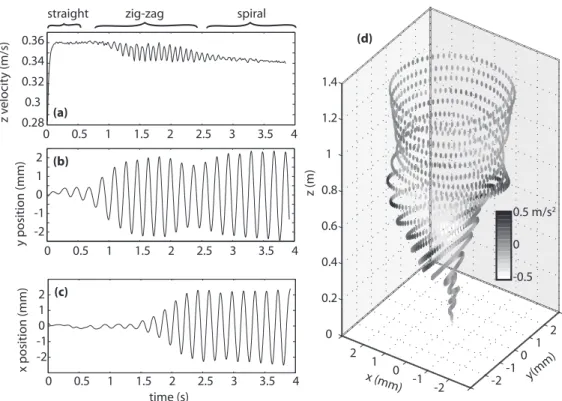
Trajectories were recorded for over 20 bubbles. From the vertical speed and horizontal position data we may re-construct the entire three dimensional trajectory for each bubble as demonstrated in Fig. 3. The bubble in Fig. 3 is 1.12 mm in radius at atmospheric pressure. This example clearly demonstrates the three different types of behavior exhibited by the bubbles in the size range of our investi-gation. Just after the bubble is generated it accelerates quickly to its terminal speed. It rises for a short time in a nearly straight path. For a large enough bubble, the rectilinear rise soon becomes unstable to a zigzag mo-tion. These oscillations are confined to a vertical plane (y-z plane in Fig. 3). The path then evolves into a spi-ral. A smooth transition occurs from zigzag to elliptical spiral, and finally to a circular spiral. This transition is shown in Fig. 4, where the trajectory is projected onto a horizontal plane.
III. FORCES ON BUBBLES
The equations of motion for a rigid body moving through a fluid at rest were established in the context of potential flow theory more than a century ago by Kirch-hoff (see chapter VI in [13]). Like in other analytical approaches to understanding bubble dynamics, potential flow theory describes the gross features, but regions of the flow with vorticity must be accounted for in order to make precise predictions. Kirchhoff’s equations have been generalized to the case of viscous, rotational flow [12] and, more recently, used in numerical work [22, 23] to investigate the behavior of freely rising bubbles with a fixed shape. The numerical work revealed the same zigzagging and spiraling paths as we and others have
ob-served experimentally as well as quantitative agreement with path oscillation amplitudes and frequencies. These results strongly suggest that shape changes to the bubble do not play a critical role in the dynamics. Based on this result and experimental observations [10] of steady bub-ble shapes for the size range we study, we assume that bubble shape is fixed and use the generalized Kirchhoff equations. (We note that de Vries et al. [8] report that zigzagging bubbles may have a slightly oscillating shape. We will address the consequences of this possibility for our measurement uncertainty later in section V.)
A. Equations of motion
The Kirchhoff equations govern the six degrees of free-dom necessary to completely specify the angular velocity Ω and the linear velocity U of a body (eqns. 8 and 7 below). Although the Kirchhoff equations are well estab-lished, we will revisit the main features of the derivation of the equation for velocity U in order to clarify the na-ture of the equations and emphasize the proper use of reference frames and coordinate systems.
First, recall that with an expression for the kinetic en-ergy T and potential enen-ergy U of the entire system in terms of only the bubble motion, one may derive equa-tions of motion for the bubble using Lagrange’s formal-ism. The system lagrangian is L = T − U and the equa-tions of motion are
d dt µ ∂L ∂UL n ¶ − ∂L ∂XL n = FnL. (2)
where the superscript L indicates that the variables are expressed in a lab-fixed (Galilean) coordinate system, XL
is the bubble position, and FL are the forces acting on
the bubble which are not expressed in the potential en-ergy term. The potential enen-ergy is simply U = −ρV gz. The kinetic energy is T = Tliquid+ Tbubble≈ Tliquid, since
the bubble’s mass is much smaller than that of the fluid it sets in motion. If the bubble is far from the boundaries of the fluid domain, T is generally a quadratic function de-pending only on Ω and U (see [13] for potential flow case and [12] for more general treatment). For an ellipsoidal body like our bubbles,
T = UiLALijUjL+ ΩLiDLijΩLj, (3)
where AL and DL are called the added mass tensor and
added rotational inertia tensors. If the bubble’s motion is rectilinear, then AL and DL are constant in time,
de-pending only on the bubble shape. When the bubble orientation changes with time, AL and DL become time
dependent as well. This point is clarified when AL ijUjL
is interpreted as the linear momentum imparted to the fluid in the i direction due to the motion of the bubble in the j direction. The equations of motion are then
d dt ¡ ALmnUnL ¢ = FnL+ FBnL , (4)
z (m) x (mm) y(mm) z ve loc it y (m/s) y p osition (mm) x p osition (mm)
straight zig-zag spiral
time (s) 0 0.5 1 1.5 2 2.5 3 3.5 4 0.28 0.3 0.32 0.34 0.36 (a) (d) 0 0.5 1 1.5 2 2.5 3 3.5 4 -2 -1 0 1 2 (b) 0 0.5 1 1.5 2 2.5 3 3.5 4 -2 -1 0 1 2 (c) -2-1 0 1 2 -2 -1 0 1 2 0 0.2 0.4 0.6 0.8 1 1.2 1.4 0.5 m/s2 -0.5 0
FIG. 3: Example trajectory of a 1.12 mm radius bubble (at 1 atm). (a) Vertical component of velocity as measured with ultrasound technique, (b) y position from camera data, (c) x position from camera data, and (d) three dimensional reconstruction of full trajectory with grayscale indicating magnitude of acceleration. The bubble begins rising straight, followed by zigzag motion in the (y, z) plane with oscillating velcocity, followed by a three-dimensional spiral motion with steady velocity.
-2 -1 0 1 2 -2 -1 0 1 2 x (mm) y (mm)
FIG. 4: Projection of a bubble trajectory onto a horizontal plane during the transition from zigzag to spiral. The bubble radius is 1.12 mm at 1 atm. The time step between plotted points is 8 ms.
where FL
B = (0, 0, ρV g) is the buoyancy force resulting
from the potential energy term.
It is convenient to recast this equation in terms of quantities which are projected onto a bubble-fixed coordi-nate system, for example Ui= RijUjL. The components
of the orthogonal projection operator R are the direction
cosines, which define the orientation of the bubble with respect the the lab-fixed coordinates. Then equation 4 becomes, d dt ¡ R−1 mlAljRjkR−1knUn ¢ = R−1 mnFn+ R−1mnFBn, (5)
where A is now time independent. Using the fact that the time derivative of Rij is Rrj²irsΩs, where ² is the
permutation tensor, the resulting equation is
R−1 mlAlj dUj dt +AljUjR −1 mr²rslΩs= R−1mnFn+R−1mnFBn. (6)
Multiplying this result by Rim and relabelling some
in-dices, we have Kirchhoff’s equation for the bubble veloc-ity,
AijdUj
dt + ²ijkΩjAklUl= Fi+ FBi. (7)
Following a similar procedure, one may obtain Kirch-hoff’s equation for the angular velocity,
DijdΩj
dt + ²ijkΩjDklΩl+ ²ijkUjAklUl= Γi. (8)
The bubble-fixed coordinate system mentioned above is precisely defined as follows. The 1-direction is always parallel to the velocity vector of the bubble. The 2-direction is at a right angle to the 1-2-direction. It is de-fined such that the 1-2 plane contains both the velocity
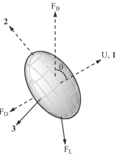
U, 1 2 FB FD 3 FL θ
FIG. 5: Diagram of the coordinate system, velocity U , pitch
angle θ, and external forces (FB, FD, FL) present for a
spi-raling bubble. The dashed lines lie in the 1-2 plane.
and the buoyancy force vector and the positive direction coincides with the 2-component of buoyancy. Finally, the 3-direction is orthogonal to the 1 and 2-directions and, hence, is always purely horizontal. This coordinate sys-tem is right-handed and cartesian as illustrated in Fig. 5. With this choice of coordinates, U = (U, 0, 0), A and D are diagonal.
B. Hydrodynamic forces and torques
For an air bubble rising through still water, the forces F, by assumption, include only drag and lift. Drag represents those forces parallel to the bubble trajectory which cannot be accounted for by FB1and lift represents
those forces acting perpendicular to the bubble trajec-tory which cannot be accounted for by FB2. Generally
we have, F = (FD+ FB1, FL2+ FB2, FL3). History forces
are not dealt with explicitly, but rather are implicit in the time dynamics of drag and lift. The torques are assumed to be divided into a rotational drag ΓD and
a wake induced torque ΓW. With these definitions of
forces, torques, and coordinate system, the equations 7 and 8 reduce to A11dU dt = FD+ FB1, (9) Ω3A11U = FL2+ FB2, (10) −Ω2A11U = FL3, (11) D11dΩ1 dt = ΓW 1+ ΓD1, (12) D22dΩ2 dt = ΓW 2+ ΓD2, (13) D33dΩ3 dt = ΓW 3+ ΓD3. (14)
C. Straight rising bubble equation
For the size range of bubbles we study, it is has been observed in experiments and numerics that the short axis of the ellipsoidal bubble is always aligned with the ble velocity vector [8, 10, 23]. A straight rising bub-ble therefore has Ω = 0. After a short initial accelera-tion from rest, the velocity becomes steady resulting in just one simple equation to describe the motion, namely
FD= −FB1. The buoyancy FB1 = ρV g and drag is
con-ventionally of the form FD= −0.5CDπR2ρU2. For
mil-limeter sized straight rising bubbles, experimental mea-surements of the drag coefficient CD are well predicted
using Moore’s theory [18]. Moore’s result is
CD= 48
ReG(χ) +
48
Re3/2G(χ)H(χ). (15)
The first term on the right, 48G(χ)/Re results from com-puting the dissipation in the flow field predicted by po-tential flow theory for an ellipsoid with a free-slip bound-ary. The second term on the right refines the calculation accounting for the rotational flow in thin boundary layers and a long thin wake. Note that Moore’s prediction of
χ(R) does not agree with experiments [9] and therefore
one must obtain the aspect ratio empirically.
As shown in figure 3 our bubbles often exhibit a short period of straight rise before the path becomes oscilla-tory. In section IV, we will use our measurements of straight rise velocity to calculate CD and compare to
Moore’s prediction.
D. Zigzagging bubble equation
For a zigzagging bubble, the angular velocity is just the time derivative of the path pitch angle θ and is always in the 3 direction, Ω = (0, 0, ˙θ). The velocity is unsteady and motion is confined to the 1-2 plane. The resulting equations of motion are
A11dU dt = FB1+ FD, (16) A11dθ dtU = FB2+ FL2, (17) D33dθ dt = ΓD3+ ΓW 3, (18)
where the components of the buoyancy force are de-termined by our path pitch angle measurements, e.g.
FB1 = FBsin θ. The remaining forces and torques are
unknown a priori. The drag is no longer expected to match Moore’s theory since Moore’s calculation was for a closed wake and steady straight line motion. Neither condition holds for a zigzagging bubble. Similarly, no prediction exists for the 2-component of lift FL2, nor for
the torques ΓD3 and ΓW 3. However, since we know the
trajectory and FB, we may calculate FD and FL2. These
E. Spiraling bubble equation
From experimental observations we know that the speed and pitch angle of a spiralling bubble are con-stant. With path oscillation frequency f , one may de-termine the angular velocity of a spiraling bubble to be Ω = (2πf cos θ, 2πf sin θ, 0). The resulting equations of motion are 0 = FB1+ FD, (19) 0 = Fb2+ FL2, (20) A112πf U sin θ = FL3, (21) 0 = ΓD1+ ΓW 1, (22) 0 = ΓD2+ ΓW 2. (23)
As in the zigzag case, the only known force is buoyancy, which leaves lift and drag to be calculated from our mea-surements. These results are presented in section VI. We remind the reader that for all calculations of forces we account for the increasing volume and aspect ratio χ caused by the hydrostatic pressure gradient.
Although little is known about ΓDand ΓW, we
specu-late that these quantities have the potential to be useful for predicting the frequency of spiral oscillation. In the same way that the balance between buoyancy and drag sets the terminal velocity of a straight rising bubble, the balance between the wake induced torque ΓW and the
drag ΓDassociated with rotation about the bubble’s
ma-jor axis may determine the rotation rate of the bubble. For a spiralling bubble, this rotation rate is directly tied to spiral frequency as mentioned above. With analytical expressions for ΓD and ΓW, one would likely be able to
predict the path oscillation frequency.
IV. STRAIGHT RISE AND ONSET OF PATH
INSTABILITY
Let us discuss several observations of the initial mo-ments of the bubble’s ascent up to the point where the trajectory becomes unstable. First, we observe an expo-nential approach to terminal speed. Second, our mea-surements of terminal speed agree with Moore’s theory [18]. Third, as bubble size is increased the bifurcation to path instability is rather abrupt and possibly subcritical. As shown in Fig. 6 the bubble accelerates to a terminal velocity Uo within the first 200 ms of the rise. The inset
in Fig. 6 shows the velocity U subtracted from the termi-nal velocity Uoand plotted on a logarithmic scale. After
about 20 ms, the rise is well approximated by an expo-nential approach to the terminal velocity. The dashed line in the inset of Fig. 6 is the equation,
U = Uo(1 − e−t/τ), (24)
where the time constant τ = 25 ms. We interpret τ as the approximate time required for the flow around the
20 60 100 140 180 0 0.1 0.2 0.3 0.4 0 50 100 ms 10-3 10-2 10-1 100 Uo - U Uo U (m/s) time (ms)
FIG. 6: Velocity during the initial 200 ms of a bubble’s rise. The inset demonstrates the exponential approach to the ter-minal speed with a time constant of 25 ms. The bubble radius is 1.09 mm at 1 atm. dr ag c oe fficien t C D Re 600 650 700 750 0.18 0.19 0.2 0.21 0.22 0.23
FIG. 7: Comparison of our drag coefficient measurements (cir-cles) during the rectilinear part of the bubble trajectories to predictions of Moore’s theory (+).
bubble to respond to a sudden change in the bubble’s speed. This time scale will be invoked again in the next section’s discussion of zigzag dynamics.
Once the bubble has attained terminal velocity it typ-ically rises for a short period in a straight trajectory be-fore beginning to zigzag. During this constant speed, rectilinear portion of the ascent our velocity measure-ments are in agreement with Moore’s (1965) theory. In Fig. 7, we compare our measurements of the drag coef-ficient CD as a function of bubble Reynolds number to
Moore’s prediction (equation 15). The excellent agree-ment with Moore’s theory and, hence, other experiagree-ments provides additional validation of our measurement tech-niques and methods of analysis.
We observe that the height above the release point at which a bubble’s path becomes unstable varies
signifi-0.9 0.95 1 1.05 1.1 1.15 hor iz on tal sp eed (m/s) bubble radius (mm) 0 0.02 0.04 0.06 0.08 0.1 0.12 0.14
FIG. 8: Horizontal speed of bubble averaged through the in-terval 1.4 - 1.6 meters above release point. A supercritical
bi-furcation would correspond to a√R − Rcritbehavior (dashed
line).
cantly with bubble size. Small bubbles can rise straight for nearly 2 meters before becoming unstable, while larger bubbles may become unstable even before reaching terminal velocity. For those bubbles whose path becomes unstable some time after reaching terminal velocity, we determine the critical radius at the onset of oscillations is 0.97 mm. Using the approximation in eqn. 1, this corresponds to a critical aspect ratio of 2.02. As a mea-sure of the character of the bifurcation from straight to oscillating path, the average horizontal component of ve-locity between a height of 1.4 and 1.6 meters is shown for a range of bubble sizes in Fig. 8. The transition is rather abrupt as bubble size is increased. This observa-tion suggests the bifurcaobserva-tion to path instability may be subcritical (see comparison to supercritical bifurcation curve √R − Rcrit in Fig. 8). Mougin and Magnaudet
[23] also suggest that the onset of zigzag motions may be subcritical for increasing aspect ratio. Perhaps one could check for hysteresis experimentally by carefully increas-ing the hydrostatic pressure (shrinkincreas-ing the bubble size) on an already oscillating bubble.
V. ZIGZAG FORCE MEASUREMENTS
As demonstrated in figure 10a the zigzag path is a smooth sinusoid confined to one vertical plane. One im-portant observation is that the speed of the bubble os-cillates during the zigzag motion. The speed oscillations are twice the frequency of the path oscillations. The drag and lift forces also oscillate at twice the path oscillation frequency.
First, let us discuss the lift FL2 (see figure 10a). We
observe that |FL2| reaches a maximum 25-30 ms after the
maximum in bubble speed. This lag may be related to the response time τ reported in the last section. The minimum in |FL2| occurs about 25-30 ms after the
min-imum bubble speed, again suggesting the importance of the response time τ . Note that |FL2| is not zero at the
point of inflection of the path as has been suggested by other authors, rather, it is about 25 ms later. The buoy-ant force begins to accelerate the bubble again during the moments just before and after the instant when FL2= 0.
While FL2is positive the lift is aiding buoyancy to bend
the path of the bubble. The sharp drop where FL2
be-comes negative again marks the extreme points of the zigzag path where the positive 2 direction reverses by definition of our coordinate system.
We turn now to drag. We observe that the oscillations in FB1 alone cannot account for the oscillations in speed
of the zigzagging bubble. Therefore FD must oscillate
as well. Remarkably, the oscillations in FD are not as
one might expect from standard drag formulas. That is, increasing speed does not coincide with an increase in
|FD|. Rather, increasing |FD| is tied to increasing |FL2|
as is evident in figure 10a. Thus, the repeating decrease in bubble speed during the zigzag can then be attributed to both a reduction in FB1as well as an increase in |FD|.
As mentioned in section III, our measurements de-pend on the assumption of steady bubble shape. While Ellingsen and Risso [10] report steady shape, de Vries
et al. [8] suggest that the shape of zigzagging bubbles
oscillates slightly. Based on de Vries’ schlieren photos, we estimate an upper limit for changes in χ to be about 10%. Such a variation would result in 5% changes in the magnitude of FL2and no more than 1 ms changes in
time dynamics. Therefore, the above discussion would be largely unaffected by such shape changes. For spiralling bubbles de Vries agrees that the shape is steady.
VI. SPIRAL MOTION
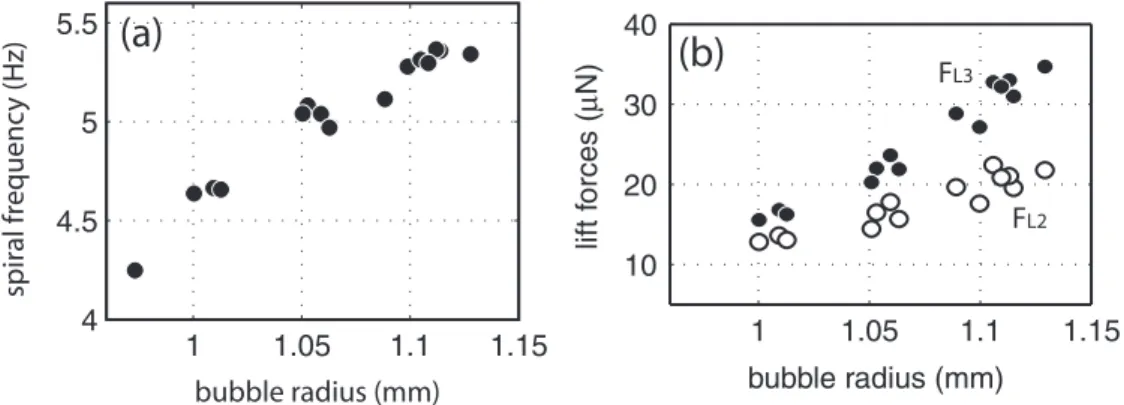
We now turn to the dynamics of spiraling bubble mo-tion. The transition to spiral motion is remarkable in sev-eral ways. First, we observe that every zigzagging path eventually becomes a spiral. The spiral may be clockwise or or counterclockwise. Bubbles may zigzag for as many as 15 and as few as 2 cycles before transitioning to the spiral. The transition to spiraling motion is not abrupt, generally developing gradually over several periods of mo-tion as demonstrated above in Fig. 4. Furthermore, the transition does not seem to behave systematically with bubble size. The frequency of path oscillations remains unchanged compared to the zigzag. This is apparent in the horizontal position data shown previously in Fig. 3. The frequency increases as bubble size is increased as shown in Fig. 11a.
The most striking change when the bubble stops zigzagging and begins to spiral is that all the forces and the bubble speed become steady. Fig. 10b shows time series of several features of a spiralling bubble. The top frame presents the component of buoyancy FB1. Since
the speed of the bubble is constant during the spiral,
0 0.5 1 1.5 2 2.5 3 3.5 -20 -10 0 10 20 lif t f or c e ( µ N) time (s)
FIG. 9: The two components of lift (FL3-dotted line, FL2- solid line) and as measured during the trajectory shown in Fig. 3. The bubble radius is 1.12 mm at 1 atm. The measurement uncertainty is about ±4 µN.
2 2.1 2.2 2.3 2.4 2.5 FB1, FD ( µ N) 0.35 0.36 speed (m/s) -5 0 5 position (mm) -20 0 lift ( µ N) time (s) x y FL3 FL2 0.35 0.36 0.37 -5 0 5 3.3 3.4 3.5 3.6 3.7 3.8 50 52 53 51 0 10 20 FB1 (µ N) speed (m/s) position (mm ) lift ( µ N) time (s) x y FL3 FL2
(a) zigzag
(b) spiral
48 52 56
FD FB1
FIG. 10: The buoyancy component tangential to the path FB1 (solid line), drag FD (dashed line), bubble velocity, horizontal
position (x and y), and lift force (solid line: FL2 and dashed line: FL3) as measured during a zigzagging trajectory (a) and a
spiraling trajectory (b). The bubble radius is 1.12 mm at 1 atm. The measurement uncertainties are ±0.5 µN for FB1and FD,
±7 mm/s for speed, ± 0.2 mm for position, and ±4 µN for lift forces.
We observe the magnitude of this drag is very nearly equal to that predicted for a bubble at the same speed using Moore’s formula. This observation is surprising since Moore’s theory is based on different flow around the bubble and the drag during the zigzag is clearly not well described by Moore’s theory. The component of lift
FL2is constant in time, balancing FB2. We observe that
FL3 is typically about twice as large as FL2, and also
constant in time. This is apparent in Figs. 9 and 10b and is quantified for a range of bubble sizes in Fig. 11b.
VII. CONCLUSIONS
We make precise three-dimensional measurements of trajectories and speed of millimeter sized air bubbles ris-ing through 2 m of still water. We use these measure-ments to calculate drag and lift forces acting on the bub-ble.
We observe that for the rectilinear portion of bubble
trajectories the measured drag matches Moore’s predic-tion. The bifurcation to path instability is abrupt and perhaps subcritical. The bifurcated state always begins as a zigzag and evolves into a spiral. We measure 10
µN oscillations in drag for a zigzagging bubble and lift
forces on both zigzagging and spiraling bubbles 10-40 µN in magnitude (buoyancy is typically 50-60 µN).
VIII. ACKNOWLEDGEMENTS
This paper benefitted from discussions at the Eu-romech colloquium 465, “Hydrodynamics of bubbly flows”. We thank Jacques Magnaudet for helpful advice on Kirchhoff equations. The skilled work of Denis Le Tourneau and Pascal Metz in building the water tank and the ultrasound device respectively is also appreciated. This work was funded by ´Ecole Normale Sup´erieure, Cen-tre National de la Recherche Scientifique, and R´egion Rhˆone-Alpes, Emergence Contract 0501551301.
1 1.05 1.1 1.15 4 4.5 5 5.5 spir al fr equenc y (Hz) bubble radius (mm) 1 1.05 1.1 1.15 10 20 30 40 lift f orces ( µ N) bubble radius (mm)
(a)
(b)
FL3 FL2FIG. 11: (a) The frequency of spiraling motion for a range of bubble sizes. The measurement is precise to within 2%. (b)
Comparison of FL2(open circles) and FL3(solid circles) for spiraling bubbles of various sizes. The measurement uncertainty is
±2 µN.
[1] N. M. Aybers and A. Tapucu, “The motion of gas bubbles rising through stagnant liquid,” W¨arme- und
Stoff¨ubertragung 2, 118 (1969).
[2] N. M. Aybers and A. Tapucu, “Studies on the drag and shape of gas bubbles rising through stagnant liquid,”
W¨arme- und Stoff¨ubertragung 2, 171 (1969).
[3] Batchelor, G. K., An introduction to fluid dynamics (Cambridge University Press, Cambridge, 1967). [4] T. B. Benjamin, “Hamiltonian theory for motions of
bub-bles in an infinite liquid,” J. Fluid Mech. 181, 349
(1984).
[5] C. Br¨ucker, “Structure and dynamics of the wake of
bub-bles and its relevance for bubble interaction,” Phys. Flu-ids 11, 1781 (1999).
[6] R. Clift, J. R. Grace, and M. E. Weber, “Bubbles, Drops, and Particles (Academic, New York, 1978).
[7] A. W. G. de Vries, “Path and wake of a rising bubble,” (PhD dissertation, University of Twente, Netherlands, 2001).
[8] A. W. G. de Vries, A. Biesheuvel, and L. van Wijngaar-den, “Notes on the path and wake of a gass bubble rising in pure water,” Int. J. Multiphase Flow 28, 1823 (2002). [9] P. C. Duineveld, “The rise velocity and shape of bubbles in pure water at high Reynolds number,” J. Fluid Mech. 292, 325 (1995).
[10] K. Ellingsen and F. Risso, “On the rise of an ellipsoidal bubble in water: oscillatory paths and liquid-induced ve-locity,” J. Fluid Mech. 440, 235 (2001).
[11] R. A. Hartunian and W. R. Sears, “On the instability of small gas bubbles moving uniformly in various liquids,” J. Fluid Mech. 3, 27 (1957).
[12] M. S. Howe, “On the force and moment on a body in an incompressible fluid, with application to rigid bodies and bubbles at low and high Reynolds numbers”, Q. J. Mech. Appl. Math. 48, 401 (1995).
[13] H. Lamb, Hydrodynamics, 6th ed. (Dover Publications, New York, 1945).
[14] L. G. Leal, “Vorticity transport and wake structure for bluff bodies at finite Reynolds number,” Phys. Fluids A 1, 124 (1989).
[15] K. Lunde and R. J. Perkins, “Observations on wakes
behind speroidal bubbles and particles,” Paper No.
FEDSM’97-3530, 1997 ASMEFED Summer Meeting, Vancouver, Canada, page 1.
[16] J. Magnaudet and I. Eames, “The motion of high-Reynolds-number bubbles in inhomogeneous flows,” Ann. Rev. Fluid Mech. 32, 659 (2000).
[17] J. Mercier, A. Lyrio, and R. Forslund, “Three dimen-sional study of the nonrectilinear trajectory of air bub-bles rising in water,” J. App. Mech. 40, 650 (1973). [18] D. W. Moore, “The velocity of rise of distorted gas
bub-bles in a liquid of small viscosity,” J. Fluid Mech. 23, 749 (1965).
[19] N. Mordant, J.-F. Pinton, and O. Michel, “Time-resolved tracking of a sound scatterer in a complex flow: Nonsta-tionary signal analysis and applications,” J. Acoust. Soc. Am. 112, 108 (2002).
[20] N. Mordant and J.-F. Pinton, “Velocity measurements of a settling sphere,” Eur. Phys. J. B 18, 343 (2000). [21] N. Mordant, P. Metz, O. Michel, and J.-F. Pinton,
“An acoustic technique for Lagrangian velocity measure-ments,” Rev. Sci. Instr. 76, 025105 (2005).
[22] G. Mougin and J. Magnaudet, “The generalized Kirch-hoff equations and their application to the interaction between a rigid body and an arbitrary time-dependent viscous flow”, Int. J. Mulitphase Flow 28, 1837 (2002). [23] G. Mougin and J. Magnaudet, “Path instability of a
ris-ing bubble.” Phys. Rev. Lett. 88, 014502 (2002). [24] G. Mougin, “Interactions entre la dynamique d’une bulle
et les instabiliti´es de son sillage,” ( PhD Dissertation, Institute National Polytechnique de Toulouse, France, 2002).
[25] C. D. Ohl, A. Tijink and A. Prosperetti, “The added mass of an expanding bubble,” J. Fluid Mech. 482, 271 (2003).
[26] A. Prosperetti, “Bubbles,” Phys. Fluids 16, 1852 (2004). [27] P. G. Saffman, “On the rise of small air bubbles in water,”
J. Fluid Mech. 1, 249 (1956).
[28] H. Sakamoto and H. Hanui, “The formation mechanism and shedding frequency of vortices from a sphere in uni-form shear flow,” J. Fluid Mech. 287, 151 (1995). [29] C. Veldhuis, Personal communications, 2005.
[30] M. Wu and M. Gharib, “Experimental studies on the shape and path of small air bubbles rising in clean water,”
![FIG. 2: Comparison of Duineveld’s [9] measurements of as- as-pect ratio and the linear model we use to estimate χ.](https://thumb-eu.123doks.com/thumbv2/123doknet/14655941.738580/3.892.127.404.78.578/fig-comparison-duineveld-measurements-ratio-linear-model-estimate.webp)