En vue de l'obtention du
DOCTORAT DE L'UNIVERSITÉ DE TOULOUSE
Délivré par :Institut National Polytechnique de Toulouse (INP Toulouse) Discipline ou spécialité :
Génie Electrique
Présentée et soutenue par :
M. GABRIEL KHOURYle mardi 16 janvier 2018
Titre :
Unité de recherche : Ecole doctorale :
Energy efficiency improvement of a squirrel-cage induction motor through
the control strategy
Génie Electrique, Electronique, Télécommunications (GEET)
Laboratoire Plasma et Conversion d'Energie (LAPLACE) Directeur(s) de Thèse :
M. MAURICE FADEL M. RAGI GHOSN
Rapporteurs :
M. BABAK NAHID-MOBARAKEH, UNIVERSITÉ LORRAINE M. GUY CLERC, UNIVERSITE LYON 1
Membre(s) du jury :
M. LUC LORON, UNIVERSITE DE NANTES, Président M. MAURICE FADEL, INP TOULOUSE, Membre
Mme FLAVIA KHATOUNIAN, UNIVERSITE ST JOSEPH DE BEYROUTH, Membre M. RAGI GHOSN, ECOLE SUPERIEURE D'INGENIEURS BEYROUTH, Membre
iii
iv
A diamond is a chunk of coal that did well under pressure Henry Kissinger
v
Acknowledgments
I would like in the first place to express my deep gratitude to my directors Pr. Maurice FADEL and Pr. Ragi GHOSN for their vital help and continuous guidance throughout the whole thesis, as well as my advisor Dr. Flavia KHATOUNIAN for always providing the necessary advices on the technical and personal levels. Calling you directors and advisors doesn’t give the complete image, since you were more like family. You were always ready to help despite all your occupations, but also always there to encourage and boost my motivation again and again.
I would also like to thank M. Mathias TIENTCHEU for providing the work with all possible information and equipment from Leroy Somer to enhance the industrial value of the results. Moreover, I would like to express my appreciation to the committee members, Pr. Guy CLERC and Pr. Babak NAHID-MOBARAKEH, for accepting to evaluate my thesis report and for sharing your valuable comments and positive feedback, as well as Pr. Luc LORON for granting me the honor of presiding the committee and presenting valued remarks.
Special thanks also to the CODIASE team in the LAPLACE laboratory, especially Pr. Pascal MAUSSION, Pr. Maria DAVID and Pr. Stephane CAUX, for their advice and help in many issues throughout the thesis during my stays at Toulouse, as well as for the welcoming and friendly environment created inside the team.
This thesis wouldn’t have been accomplished without the support of the Research Council and the CINET research center of the Université Saint-Joseph de Beyrouth (USJ), the Agence Universitaire de la Francophonie AUF, the Lebanese National Council for Scientific Research CNRS-L, the LAPLACE research center and Leroy Somer – Nidec Industry. These entities and programs are deeply thanked for supporting the thesis with all necessary funds.
In every situation through these long years, friends were an essential ingredient that kept things going. I am really thankful for each and every one for making it a pleasant experience. Thank you for my lab friends Antoine, Leopold, Abdelkader, Khaled, Pedro and Julien for sharing difficulties in Toulouse and turning them into funny stories. Very special thanks for my Lebanese friends at Toulouse Bernard, Hiba, Sabina, Sirena, Charbel, Carole… who made me always feel at home and enjoy every moment outside my country. Thank you for my ESIB friends and colleagues Melhem, Jean, Samer, Michel and all the REDOC team who accompanied every step of the process by sharing personal experience and being perfect
vi
listeners when needed! And of course, I can’t forget my old friends who were always there since before my Ph.D. and always encouraged my decisions… thank you Sergio, Elio, Mario, Eliane, Freddy, Marianne, Sarah, Christophe, Robert, Yassin, Stephan, André, Wissam… The list doesn’t end here, many are the friends who were there making my experience special, I thank you deeply.
In the end, the biggest thanks go to my dear family, Amale, Joe and Christian, who always believed in my capabilities and encouraged my ambitions especially throughout these three years, despite all the financial problems we’ve been through. For you I am so grateful, especially for my dearest Ammoula my super-mum, my weakness and my support in life.
viii
Abstract
Energy efficiency optimization of electric machines is an important research field and is part of the objectives of several international projects such as the European Commission Climate and Energy package which has set itself a 20% energy savings target by 2020, and was extended for 2030 with higher targets. Therefore, this thesis proposes an efficiency optimization method of the Induction Machine (IM) through the variation of the control parameters. To achieve this goal, the flux in the airgap is modified according to an optimal flux table computed off-line for all possible operating points.
The flux table is calculated with the best possible accuracy through an improved dynamic model of the IM, developed in these works. The latter avoids the main drawback of the classic dynamic model, by considering the effect of core losses. The core loss model established by Bertotti is used. It depends on the frequency and the amplitude of the magnetic field. The losses are then represented by a variable resistor, continuously evaluated according to the operating point.
The established optimal flux table is a function of the operating conditions in terms of torque and speed. Indeed, the results show that the flux can be optimized for torque values less than about half the rated torque, and that this threshold is influenced by the speed. The proposed optimization method is simulated, then tested for the scalar control and the field-oriented control, in order to show the genericity of the proposed approach. The validation is carried on an experimental test bench for two 5.5 kW induction motors of different efficiency standards (IE2 and IE3). The results obtained show the reduction of the losses in the motor, thus an improvement of the overall efficiency while preserving a satisfactory dynamic behavior. Consequently, the optimization of the energy efficiency is validated for the two control structures and for the two studied motors. In addition to the validation of the simulation results, the proposed approach is compared to existing methods to assess its effectiveness.
ix
Résumé
L’optimisation de l’efficacité énergétique des machines électriques constitue un domaine de recherche bien développé et fait partie des objectifs de plusieurs accords internationaux comme le projet Energie-Climat de la Commission Européenne visant l’amélioration de 20% d’efficacité pour 2020, encore étendu pour 2030 avec des objectifs plus importants. Ainsi, cette thèse propose un procédé d’optimisation du rendement du moteur asynchrone en agissant sur les paramètres du contrôle. Pour atteindre cet objectif, le flux dans l’entrefer est adapté selon un tableau de flux optimal calculé hors ligne pour tous les points de fonctionnement possibles.
Ce flux est déterminé avec le plus haut degré de précision possible en se basant sur un modèle dynamique de la machine développé dans ces travaux. Ce dernier pallie le point faible du modèle dynamique classique, en prenant en compte l’effet des pertes fer. Le modèle des pertes fer utilisé est celui de Bertotti, qui les évalue en fonction de la fréquence et de l’amplitude du champ magnétique. Les pertes sont alors représentées par une résistance variable, continuellement évaluée selon le point de fonctionnement.
Le tableau de flux optimal obtenu est fonction des conditions d’opération repérées dans le plan couple-vitesse. Ainsi l’étude montre que le flux peut être optimisé pour des valeurs de couple sensiblement inférieures à environ la moitié du couple nominal, ce seuil variant en fonction de la vitesse. La méthode d’optimisation proposée est simulée puis testée pour le contrôle scalaire et le contrôle vectoriel indirect par orientation de flux rotorique, afin de montrer la généricité de l’approche. La validation est conduite sur une maquette expérimentale d’une puissance de 5.5 kW et pour 2 machines asynchrones de générations différentes (IE2 et IE3). Les résultats obtenus montrent la réduction des pertes dans la machine et donc une amélioration du rendement global, tout en préservant un comportement dynamique satisfaisant. L’optimisation de l’efficacité énergétique est ainsi validée pour les deux structures de contrôle et pour les deux types de machine. Outre une comparaison avec la simulation, la solution proposée est comparée aux méthodes existantes afin d’en apprécier l’efficacité.
Table of Contents
Acknowledgments ... v Abstract ... viii Résumé ... ix Table of Contents ... xi List of Figures ... xvList of Tables ... xviii
List of Symbols ... xix
General Introduction ... 1
Chapter 1 Context of the Thesis ... 3
Introduction ... 4
1.1 General Context... 4
1.1.1 European Climate & Energy Package ... 4
1.1.2 Energy Efficiency Standards for Electric Motors ... 5
1.2 State of Art of Existing Induction Motors Models ... 7
1.2.1 Steady State Equivalent Circuits ... 7
1.2.2 Dynamic Model ... 9
1.2.3 Improved Dynamic Models ... 13
1.3 Models of the Main Losses ... 14
1.3.1 Copper Losses... 15
1.3.2 Mechanical Losses ... 15
1.3.3 Core Losses... 16
1.3.4 Inverter Losses ... 17
1.3.5 Summary ... 20
1.4 Energy Efficiency Optimization of the Induction Motor ... 21
1.4.1 Search Control ... 22
1.4.2 Loss Minimization Control ... 23
1.4.3 Maximum Torque per Ampere ... 24
1.4.4 Summary ... 25
Conclusion ... 25
Chapter 2 Induction Motor Model Taking Core Losses into Account ... 26
Table of Contents
xii
2.1 Model Parameters Measurement ... 27
2.1.1 Mechanical Parameters ... 27
2.1.2 Electrical Parameters ... 28
2.1.3 Core Losses Model Coefficients ... 30
2.2 Including Core Losses in the IM Model ... 31
2.2.1 Equivalent Torque Approach... 32
2.2.2 Equivalent Resistor Approach ... 32
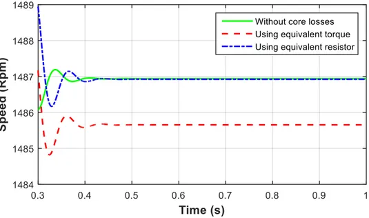
2.2.3 Summary and Analysis ... 34
2.3 Including Variable Core Losses ... 37
2.3.1 Enhancement of the Improved Dynamic Model ... 38
2.3.2 Simulation Results and Experimental Validation ... 38
Conclusion ... 39
Chapter 3 Best Efficiency Point Tracking ... 40
Introduction ... 41
3.1 Efficiency Computation ... 41
3.1.1 Improved Dynamic Model in Complex Form ... 41
3.1.2 Efficiency Equations ... 43
3.2 Efficiency Mapping ... 45
3.2.1 Energy Efficiency Curves ... 45
3.2.2 Energy Efficiency Plans ... 48
3.3 Efficiency Optimization Approach ... 50
3.3.1 Optimal Flux ... 50
3.3.2 Load Torque Observer ... 53
Conclusion ... 55
Chapter 4 Control Systems Optimization... 56
Introduction ... 57
4.1 Scalar Control Optimization... 57
4.1.1 Classic Scalar Control Structure ... 57
4.1.2 Optimized Scalar Control ... 59
4.1.3 Simulation and analysis ... 61
Table of Contents
xiii
4.2.1 Classic field-oriented Control Structure ... 67
4.2.2 Optimized field-oriented Control ... 73
4.2.3 Simulation and analysis ... 73
Conclusion ... 78
Chapter 5 Experimental Validations ... 79
Introduction ... 80
5.1 Experimental Test Bench ... 80
5.1.1 Global Test Bench ... 80
5.1.2 Power Elements ... 81
5.1.3 Sensors and Control System ... 85
5.1.4 Operating Points Validation ... 87
5.2 Optimized Scalar Control Tests ... 87
5.2.1 Setup ... 88
5.2.2 Experimental Results ... 89
5.3 Optimized Field-oriented Control Tests ... 96
5.3.1 Setup ... 96
5.3.2 Experimental Results ... 98
5.4 Comparison with the Existing Optimization Methods ... 104
5.4.1 Methods in Literature ... 104
5.4.2 Industrial Method ... 106
5.5 IE3 motor tests ... 110
5.5.1 Tested Motor... 110
5.5.2 Experimental Results ... 111
5.5.3 Comparison with the IE2 Motor ... 114
Conclusion ... 115
General Conclusion ... 116
Résumé Long en Français ... 119
Introduction ... 119
Chapitre 1 Contexte de la thèse ... 120
1.1 Contexte Général ... 120
Table of Contents
xiv
1.3 Modèles des Pertes Principales ... 124
1.4 Amélioration de l’Efficacité Energétique de la Machine Asynchrone ... 125
Chapitre 2 Modèle dynamique prenant en compte les pertes fer... 125
2.1 Détermination des Paramètres de la Machine ... 126
2.2 Prise en Compte des Pertes Fer ... 126
2.3 Prise en Compte du Caractère Variable des Pertes Fer ... 129
Chapitre 3 Rendement Optimal ... 130
3.1 Calcul du Rendement ... 130
3.2 Cartographie du Rendement ... 130
3.3 Approche d’Optimisation ... 132
Chapitre 4 Contrôles Optimisés ... 133
4.1 Contrôle Scalaire Optimisé ... 133
4.2 Contrôle Vectoriel Optimisé ... 134
Chapitre 5 Validation Expérimentale ... 139
5.1 Montage Expérimental ... 139
5.2 Validation des Contrôles Optimisés ... 140
5.3 Comparaison avec les Méthodes Existantes... 143
Conclusion ... 145
References ... 147
List of Publications ... 154
Appendix A – Efficiency and Flux Calculation Methods ... 155
Appendix B – Motors Characteristics ... 157
List of Figures
Fig. 1.1. IE efficiency classification according to IEC 60034-30-1:2014 standard [4] ... 6
Fig. 1.2. IM partial leakage inductances equivalent circuit referred to the stator ... 8
Fig. 1.3. IM global leakage inductance equivalent circuit referred to the stator ... 8
Fig. 1.4. Dynamic model representation including core losses through equivalent resistor and inductance ... 13
Fig. 1.5. d-q dynamic model representation including core losses through equivalent resistor ... 14
Fig. 1.6. Losses in an inverter fed squirrel-cage induction motor system ... 15
Fig. 1.7. Comparison between SC and intelligent SC flux reference ... 23
Fig. 1.8. MTPA strategy reference curves for a 7.5kW IM ... 24
Fig. 2.1. IM speed variation in zero-load deceleration experiment ... 28
Fig. 2.2. IM dynamic model schematic representation ... 33
Fig. 2.3. IM dynamic model schematic representation including core losses through an equivalent resistor ... 33
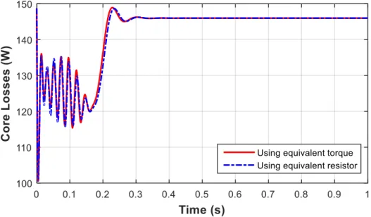
Fig. 2.4. Simulated core losses in a direct start-up test at 0.25p.u. load ... 35
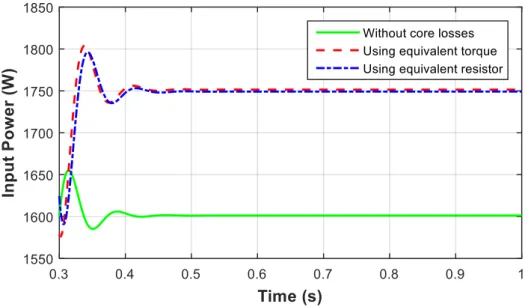
Fig. 2.5. Simulated input power in a direct start-up test at 0.25p.u. load ... 36
Fig. 2.6. Simulated electromagnetic torque in a direct start-up test at 0.25p.u. load ... 37
Fig. 2.7. Simulated speed in a direct start-up test at 0.25p.u. load ... 37
Fig. 2.8. Simulated and experimental core losses ... 38
Fig. 3.1. Energy efficiency variations at 0.1p.u. torque ... 46
Fig. 3.2. Energy efficiency variations at 0.3p.u. torque ... 46
Fig. 3.3. Energy efficiency variations at 0.5p.u. torque ... 47
Fig. 3.4. Energy efficiency variations at 1p.u. torque ... 47
Fig. 3.5. Energy efficiency variations in flux-speed plan at 0.1p.u. torque ... 48
Fig. 3.6. Energy efficiency variations in flux-speed plan at 0.3p.u. torque ... 48
Fig. 3.7. Energy efficiency variations in flux-speed plan at 0.5p.u. torque ... 49
Fig. 3.8. Energy efficiency variations in flux-speed plan at 1p.u. torque ... 49
Fig. 3.9. Optimal stator flux values per load torque and speed requirements ... 51
Fig. 3.10. Optimal rotor flux values per load torque and speed requirements ... 52
Fig. 3.11. First order Luenberger load torque observer ... 54
Fig. 3.12. Torque observer simulation ... 55
Fig. 4.1. Classic Scalar Control Structure ... 58
Fig. 4.2. Optimized Scalar Control Structure ... 61
Fig. 4.3. Simulation of the inverter PWM ... 62
Fig. 4.4. Optimized scalar control – stator flux reference and actual values ... 63
Fig. 4.5. Scalar control – speed and electromagnetic torque ... 64
Fig. 4.6. Scalar control – Input power and losses. a- copper losses, b- core losses, c- input power, d- energy efficiency ... 65
Fig. 4.7. Scalar control – Input power (zoom) ... 66
List of Figures
xvi
Fig. 4.9. Scalar control – Energy efficiency (zoom) ... 67
Fig. 4.10. Basic indirect field-oriented control structure ... 69
Fig. 4.11. FOC speed loop ... 71
Fig. 4.12. Flux reference reduction ... 72
Fig. 4.13. Approximate IM schematic representation taking core losses into account ... 72
Fig. 4.14. Flux reference generator – optimized FOC ... 73
Fig. 4.15. Optimized field-oriented control – rotor flux reference and actual values ... 74
Fig. 4.16. Field-oriented control – speed and electromagnetic torque ... 75
Fig. 4.17. Field-oriented control – Input power and losses. a- copper losses, b- core losses, c- input power, d- energy efficiency ... 76
Fig. 4.18. Field-oriented control – Input power (zoom) ... 77
Fig. 4.19. Field-oriented control – Energy efficiency ... 77
Fig. 4.20. Field-oriented control – Energy efficiency (zoom) ... 78
Fig. 5.1. Test bench structure ... 81
Fig. 5.2. Test bench ... 81
Fig. 5.3. Semikron inverter. a- didactic block, b- IGBT SKM 50 module, c- SKHI 22 driver83 Fig. 5.4. Leroy Somer IE2 squirrel-cage induction motor LSES 132... 83
Fig. 5.5. Front panel of the dSpace controller... 86
Fig. 5.6. Experimental validation operating points. a- industrial test points, b- effective test points ... 87
Fig. 5.7. Optimized scalar control block diagram ... 89
Fig. 5.8. Experimental scalar control optimization with variable load profile. a- load torque, b- stator flux, c- energy efficiency ... 90
Fig. 5.9. Optimized scalar control operating conditions. a- flux reference, b- speed, electromagnetic and load torque ... 92
Fig. 5.10. Simulated and experimental optimized scalar control results. a- copper losses, b- core losses, c- input power, d- energy efficiency ... 93
Fig. 5.11. Simulated and experimental optimized scalar control results (zoom). a- input power, b- energy efficiency ... 94
Fig. 5.12. Optimized scalar control efficiency increase - IE2 motor ... 96
Fig. 5.13. Optimized field-oriented control block diagram ... 97
Fig. 5.14. Experimental FOC optimization with variable load profile. a- load torque, b- stator flux, c- energy efficiency ... 98
Fig. 5.15. Optimized FOC operating conditions. a- rotor flux, b- speed and torque ... 99
Fig. 5.16. Simulated and experimental optimized FOC results. a- copper losses, b- core losses, c- input power, d- energy efficiency ... 100
Fig. 5.17. Simulated and experimental optimized FOC results (zoom). a- input power, b- energy efficiency ... 101
Fig. 5.18. Optimized FOC efficiency increase - IE2 motor ... 102
Fig. 5.19. Flux variation test – 0.5p.u. speed, 0.25p.u. torque. a- rotor flux, b- energy efficiency ... 103
List of Figures
xvii
Fig. 5.20. Search control technique. a- rotor flux, b- energy efficiency ... 104
Fig. 5.21. Intelligent search control technique. a- rotor flux, b- energy efficiency ... 105
Fig. 5.22. Proposed optimization technique. a- rotor flux, b- energy efficiency ... 106
Fig. 5.23. Industrial drives optimization curve ... 107
Fig. 5.24. Comparison with the industrial optimization – 0.25p.u. speed, 0.5p.u. torque. a- flux, b- energy efficiency ... 108
Fig. 5.25. Comparison with the industrial optimization - 1p.u. speed, 0.25p.u. torque. a- flux, b- energy efficiency ... 108
Fig. 5.26. Comparison with the industrial optimization – 0.9p.u. speed, 0.5p.u. torque. a- flux, b- energy efficiency ... 109
Fig. 5.27. Comparison with the industrial optimization – efficiency improvements ... 110
Fig. 5.28. Optimized scalar control efficiency increase – IE3 motor ... 113
Fig. 5.29. Optimized FOC efficiency increase – IE3 motor ... 114
Fig. 5.30. Comparison IE2 and IE3 motors – 0.9p.u. speed, 0.25p.u. torque. a- IE2 motor, b- IE3 motor ... 115
Fig. 1.1. Schéma monophasé étoile équivalent ramené au stator de la machine asynchrone 122 Fig. 2.1. Représentation schématique du modèle dynamique de la machine asynchrone prenant en compte les pertes fer ... 127
Fig. 2.2. Simulation des modèles dynamiques proposés. a- vitesse, b- couple électromagnétique ... 128
Fig. 2.3. Pertes fer expérimentales et simulées ... 129
Fig. 3.1. Courbes de rendement. a- couple 0.1p.u., b- couple 1p.u. Abaques de rendement dans le plan flux-vitesse. c- couple 0.1p.u., d- couple 1p.u. ... 131
Fig. 3.2. Abaque de flux statorique optimal... 132
Fig. 4.1. Contrôle scalaire optimisé ... 134
Fig. 4.2. Contrôle vectoriel indirect optimisé ... 136
Fig. 4.3. Simulation de l’optimisation du flux rotorique dans le cas du contrôle vectoriel ... 137
Fig. 4.4. Simulation de l’effet de l’optimisation proposée sur la vitesse et le couple électromagnétique ... 137
Fig. 4.5. Simulation de l’effet de l’optimisation proposée sur les pertes et la puissance absorbée. a- pertes Joule, b- pertes fer, c- puissance absorbée, d- pertes onduleur ... 138
Fig. 4.6. Simulation de l’effet de l’optimisation proposée sur le rendement ... 139
Fig. 5.1. Montage expérimental ... 140
Fig. 5.2. Résultats expérimentaux de l’essai de variation de charge avec et sans optimisation. a- couple de charge, b- flux rotorique, c- rendement. ... 141
Fig. 5.3. Résultats expérimentaux d’augmentation du rendement ... 142
Fig. 5.4. Résultats expérimentaux de variation du flux ... 143
Fig. 5.5. Résultats expérimentaux d’amélioration du rendement par rapport à l’approche d’optimisation industrielle ... 144
List of Tables
Table 1.1. Conduction voltage drops per inverter leg ... 18
Table 1.2. Power losses ... 21
Table 3.1. Optimal stator flux table – IE2 motor ... 51
Table 3.2. Optimal rotor flux table – IE2 motor ... 52
Table 5.1. Studied IE2 motor parameters ... 84
Table 5.2. Optimized scalar control experimental vs simulated efficiency error - IE2 motor 95 Table 5.3. Optimized scalar control efficiency increase - IE2 motor ... 95
Table 5.4. Optimized FOC experimental vs simulated efficiency error - IE2 motor ... 102
Table 5.5. Optimized FOC efficiency increase - IE2 motor ... 102
Table 5.6. Comparison with the industrial optimization – efficiency improvements ... 109
Table 5.7. Studied IE3 motor parameters ... 111
Table 5.8. Optimal stator flux table – IE3 motor ... 112
Table 5.9. Optimal rotor flux table – IE3 motor ... 112
Table 5.10. Optimized scalar control efficiency increase – IE3 motor ... 113
Table 5.11. Optimized FOC efficiency increase – IE3 motor ... 113
Tableau 3.1. Flux statorique optimal ... 132
Table 1. Studied IE2 motor parameters ... 157
Table 2. Studied IE3 motor parameters ... 157
List of Symbols
magnetic field variable core losses branch subscript , rotating reference frame subscripts
voltage frequency
� viscous friction coefficient
current variable RMS current voltage total motor and load inertia
eddy currents effect core losses coefficient
� excess core losses coefficient
� hysteresis effect core losses coefficient
Luenberger factor
partial stator leakage inductance
′ partial rotor leakage inductance referred to the stator eddy currents inductance
magnetizing inductance of the partial leakage inductances equivalent circuit
magnetizing inductance of the global leakage inductance equivalent circuit stator self-inductance
rotor self-inductance
magnetizing branch subscript stator-rotor mutual inductance
′ global leakage inductance referred to the stator core losses
� input active power
� input reactive power
mechanical losses
� rotor copper losses
� stator copper losses
resistance of a stator phase winding
′ resistance of a rotor phase winding referred to the stator core losses equivalent resistance
short-circuit resistor of the IM equivalent circuit rotor resistance
stator resistance
number of pole pairs of the motor , stator and rotor subscripts
dry friction torque
core losses equivalent torque electromagnetic torque load torque
List of Symbols
xx
̂ observed load torque
voltage variable
conduction losses voltage drop switching losses voltage drop RMS stator voltage
� switching frequency triangular voltage
VSD Variable Speed Drive
̅ variable phasor: ̅ = +
short-circuit reactance of the IM equivalent circuit short-circuit impedance of the IM equivalent circuit , stationary reference frame subscripts
� energy efficiency
� motor dispersion coefficient � = − 2
∅ flux variable
� mechanical speed of the rotor � electrical speed of the rotor
� angular speed of the rotating frame � angular frequency of the rotor currents � angular frequency of the stator currents
General Introduction
The present thesis aims to optimize the energy efficiency of a squirrel-cage induction motor by acting on the control strategy and fixing the best efficiency operating point.
Energy efficiency optimization has become nowadays the goal of a lot of research, especially for electrical systems, which constitute an essential domain and have significant energy requirements. The European Commission for instance, has set energy efficiency targets, and standards to be reached throughout 2020 and 2030, thus motivating further developments in the field. Indeed, this work is a contribution in fulfilling the objectives of the European project by acting on the energy efficiency optimization of electrical structures.
The squirrel-cage Induction Motor (IM) is a main element among electrical systems since it is one of the most used motors in industry for the simplicity of its installation and use. Indeed, the IM is found in a wide number of industries like construction, transportation, HVAC, packaging, raw materials exploitation, etc. Therefore, the present study is focused on this type of motors.
On the other hand, control systems have a significant role in enhancing the energy efficiency and are therefore an important tool in this domain. Several types of control structures can be used. This thesis focuses on the scalar control, which is used by a wide number of applications for its simplicity, as well as the field-oriented control also widely used for its precision and stability. The energy optimization of these control structures is achieved by acting on the flux reference to change the operating point of the motor.
In order to conduct an efficiency study and to identify the optimal flux, it is essential to analyze the main losses in the system. However, the greater number of studies carried on the induction motor take into consideration copper and mechanical losses, while omitting the core losses because of the complexity of their estimation. Nevertheless, these are main losses which must be addressed to reach the best possible accuracy. For this purpose, the commonly used IM dynamic model that omits core losses is updated in this study to match the requirements.
Several improvement methods relative to efficiency optimization are discussed in literature, and are proved to optimize the efficiency. These methods however lack accuracy in some cases and lead to unsatisfactory dynamic performances in other cases. They are nevertheless used as comparative optimization techniques in this study.
In this thesis, an improved dynamic model of the IM introducing the core losses effect is established, considering their dependency on frequency and magnetic field. This model is then
General Introduction
2
used to analyze the efficiency variations and compute the optimal flux values which are stored in a look-up table. The latter is used to optimize both scalar and field-oriented control structures to reach the best efficiency point. The flux reference is modified throughout the motor operation. In the end, results are simulated and experimentally validated and compared to existing optimization methods to show the originality and effectiveness of the proposed solution. This approach has an industrial vocation for rapid implementation on several types of motors.
In the first chapter, the European Commission project headlines are described especially concerning the efficiency standards, then an overview of the existing induction motor models is presented, as well as a list of the system losses models necessary for the study. A state-of-art of the optimization methods found in literature is presented at the end, showing the advance in the field and the weaknesses to be resolved in the proposed approach.
In the second chapter, the improved dynamic model of the IM taking into account the effect of core losses is presented, along with the necessary parameters measurements. Two methods are presented and compared, then the chosen approach is enhanced by considering the magnetic field and frequency effect of the core losses to improve accuracy.
In the third chapter, the improved dynamic model is used to compute the optimal stator and rotor flux values, which are stored in the look-up table, to be used later in the control structures. Efficiency variations are observed in torque-speed planes to analyze the effect of the operating conditions in terms of flux, torque and speed on the efficiency.
In the fourth chapter, the optimal flux look-up table is used to enhance the scalar and field-oriented controls. The classic and improved control structures are described, and simulation results are presented to confirm the predicted efficiency increase compared to the classic structures results.
In the fifth chapter, experimental validations are presented. A test bench built in the LAPLACE laboratory is described in this section, as well as the series of tests carried to validate the results of both improved control structures. In addition, tests done with existing optimization methods and on a second motor compliant with a better efficiency standard, are presented to prove the originality and effectiveness of the proposed approach.
Chapter 1 Context of the Thesis
Table of Contents
Introduction ... 4 1.1 General Context... 4 1.1.1 European Climate & Energy Package ... 4 1.1.2 Energy Efficiency Standards for Electric Motors ... 5 1.2 State of Art of Existing Induction Motors Models ... 7 1.2.1 Steady State Equivalent Circuits ... 7 1.2.2 Dynamic Model ... 9 1.2.3 Improved Dynamic Models ... 13 1.3 Models of the Main Losses ... 14 1.3.1 Copper Losses... 15 1.3.2 Mechanical Losses ... 15 1.3.3 Core Losses... 16 1.3.4 Inverter Losses ... 17 1.4 Energy Efficiency Optimization of the Induction Motor ... 21 1.4.1 Search Control ... 22 1.4.2 Loss Minimization Control ... 23 1.4.3 Maximum Torque per Ampere ... 24 1.4.4 Summary ... 25 Conclusion ... 25
Chapter 1. Context of the thesis
4
Introduction
The optimization of energy efficiency in industrial applications using electrical motors is a favorite area for studies associated to international projects and standards promoting ‘green’ energies. The squirrel-cage induction motor is one of the most studied systems and the object of this thesis, since it is widely used in industry and constitutes an important source of energy consumption. Therefore, several optimization techniques of the IM are proposed in literature to optimize their efficiency. These studies require the use of mathematical models of the IM and the losses that occur in the system.
In the present chapter, the general context of this work is presented as part of the European Commission project goals. The progress in the field is also detailed in terms of motor and power losses models as well as the state-of-art of the optimization techniques leading to the method proposed in the thesis, and used as comparative approaches in the rest of the study.
1.1 General Context
Energy efficiency optimization is the main scope of much research nowadays because of the climate changes and the necessity to reduce energy consumption and promote sustainable strategies. For this purpose, the European Climate and Energy package of the European Commission has been established in 2008 along with several standards and projects.
1.1.1 European Climate & Energy Package
The consequences of the 2008 worldwide economic crisis were severe for the progress of many countries, and exposed the weaknesses in their economic structures, which required an immediate intervention to ensure a quick recovery. Therefore, the European Union took the initiative in the ‘Europe 2020 strategy’ [1] and set objectives to be reached by 2020 at different levels with three priorities: smart, sustainable and inclusive growth.
To this end, a list of headline targets was imposed to promote research and education, improve the economy, reduce poverty and unemployment, and deal with the climate change challenges by encouraging sustainable energies and optimizing energy efficiency. The 3*20
Chapter 1. Context of the thesis
5
Climate & Energy package is established to define the three main objectives of the sustainable energy program as shown below:
• Reduce the greenhouse gas emissions by at least 20% compared to 1990 levels or by 30%, according to the capabilities of the countries,
• Increase by 20% the use of renewable energy sources for the final energy consumption,
• Reach a 20% increase in energy efficiency of electric structures.
The scopes of the European project are mutually reinforced, in a way that each objective helps in achieving the others. For instance, the 3*20 package contributes in adding around 1 million new jobs and increasing the GDP by using the European energy market. Moreover, a major factor for limiting the greenhouse gas emissions lies in the efficiency optimization of the energy resources, which makes the latter an important research domain aiming to reach the climate/energy set goals.
Further to the above, the Climate and Energy package is being updated continuously [2] and is not only limited to 2020. Targets have already been set for 2030 with 40% cuts in greenhouse gas emissions (from 1990 levels), 27% share for renewable energy and 27% improvement in energy efficiency.
The present work is a contribution in the third objective of the Climate & Energy package, with the aim to optimize the energy efficiency of induction motors. For this purpose, the targets defined by the European Commission in terms of IM efficiency standards are explored.
1.1.2 Energy Efficiency Standards for Electric Motors
Since most of the electrical structures are based on electric motors working for several hours per day, specific guidelines have been established by the European Commission [3] fixing efficiency targets for manufactured three-phase squirrel-cage induction motors which:
• have 2 to 6 poles,
• have a rated voltage up to 1000 V,
Chapter 1. Context of the thesis
6 • are rated for continuous duty operation.
Efficiency standards IE1 to IE4 were set by the International Electrotechnical Commission (IEC) in the IEC 60034-30-1 standard [4], to classify the motors according to the following scale:
• IE1: standard efficiency, • IE2: high efficiency, • IE3: premium efficiency, • IE4: super premium efficiency.
This classification is presented for instance in Fig 1.1 for 4-pole 50Hz induction motors, showing the efficiency values corresponding to each class.
Fig 1.1. IE efficiency classification according to IEC 60034-30-1:2014 standard [4]
In order to meet the 3*20 package objectives by 2020 in terms of energy efficiency, the European Commission set three stages for motors efficiency progress through the decade:
• Stage 1, 16 June 2011: Motors must meet IE2 efficiency level,
• Stage 2, 1 January 2015: Motors with rated output of 7.5 to 375kW must meet either IE3 or IE2 if equipped with Variable Speed Drives (VSD),
• Stage 3, 1 January 2017: Motors with rated output of 0.75 to 375kW must meet either IE3 or IE2 if equipped with VSDs.
Chapter 1. Context of the thesis
7
The IE4 efficiency standard shown in Fig 1.1 is not part of the actual scopes of the commission program but is defined for future stages. The proposed stages and standards are respected by the motors and drives manufacturers, in addition to the researches and projects which are initiated to study the performance of high-efficient motors [5], and to improve the energy efficiency to meet the 3*20 package for 2020 and its extension to 2030.
Calculations and results obtained in this thesis are based on an IE2 high-efficiency IM, then compared with the results obtained by an IE3 premium-efficiency IM, to show the effect of the proposed method on the energy efficiency, according to the motor standard. Hence, a first step for carrying a study on the IM is by defining an accurate mathematical model, which predicts the motor performance according to the required operating conditions.
1.2 State of Art of Existing Induction Motors Models
An essential part of the studies on electric motors is based on their modeling, which must be as similar as possible to the real motor performance, in order to predict the outcomes of any application or control. In the case of squirrel-cage induction motors, several types of models are developed in literature based on different assumptions and used according to the operating conditions (transient or steady state).
1.2.1 Steady State Equivalent Circuits
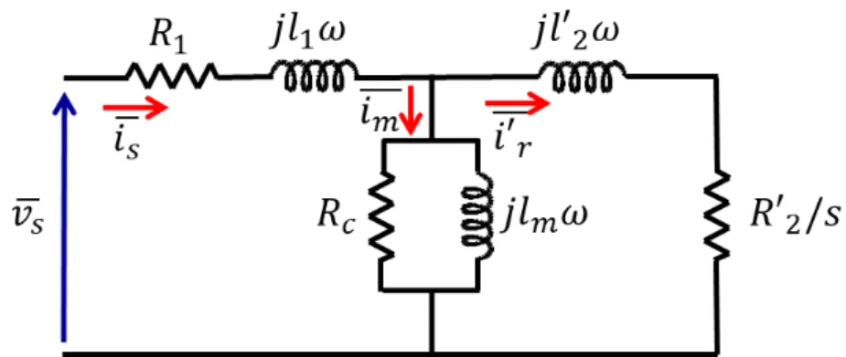
The basic representation of the induction motor is the steady-state equivalent circuit referred to the stator and composed by the main electric parameters of the motor [6]-[9]. These parameters represent the stator and rotor resistors, the leakage and magnetizing inductances, and the core losses equivalent resistor. The model predicts the motor performance at steady-state in terms of voltages, currents and stator flux values, as well as electric losses. The obtained values are referred to the stator by applying the motor stator-rotor voltage ratio.
There are two main types of equivalent circuits [10] for squirrel-cage induction motors which differ by the model used to represent the magnetic flux leakage. The first type uses the partial leakage method, leading to an equivalent circuit where both stator and rotor leakage
Chapter 1. Context of the thesis
8
inductances are presented as shown in Fig. 1.2, and the second type is the global leakage method leading to an equivalent circuit with one global leakage inductance as in Fig. 1.3.
Fig. 1.2. IM partial leakage inductances equivalent circuit referred to the stator
Fig. 1.3. IM global leakage inductance equivalent circuit referred to the stator
The presented motor parameters are defined as follows: resistance of a stator phase winding
′ resistance of a rotor phase winding referred to the stator core losses equivalent resistor
partial stator leakage inductance
′ partial rotor leakage inductance referred to the stator
magnetizing inductance of the partial leakage inductances equivalent circuit ′ global leakage inductance referred to the stator
Chapter 1. Context of the thesis
9
̅ represents the stator voltage, �̅ the stator current, �′̅̅̅ the rotor current referred to the stator, �̅̅̅ the magnetizing current, � the stator voltage angular frequency and the slip of the IM.
The presented equivalent circuits both give an accurate model of the IM in steady state, and the parameters are measured through standard tests. The partial leakage inductances model is a more realistic representation of the IM, yet a more complicated one. Therefore, since both models give similar and accurate results, the global leakage inductances equivalent circuit is used in this study to reduce calculation complexity and focus on the main scope of this work.
1.2.2 Dynamic Model
Further to the steady state equivalent model, the transient state performance of the IM is predicted by a series of electrical and mechanical equations forming the dynamic model [11]-[17] which evaluates the voltage, flux and speed variations under any operating conditions. The variables of this model are writen in the stationary reference frame / obtained by applying the Concordia transform to the corresponding three-phase / / components, as shown in (1.1). [ ] = √ [ − . − . √ −√ √ √ √ ] [ ] (1.1)
The well-known dynamic model of the squirrel-cage induction motor is thus detailed in (1.2) to (1.11).
• Stator electrical equations
= + ∅ (1.2)
Chapter 1. Context of the thesis
10 • Rotor electrical equations
= + ∅ + �∅ (1.4)
= + ∅ − �∅ (1.5)
• Stator flux equations
∅ = + (1.6)
∅ = + (1.7)
• Rotor flux equations
∅ = + (1.8) ∅ = + (1.9) • Mechanical equation � = − �� − � − (1.10) = � (∅ ∅ − ∅ ∅ ) (1.11)
This model contains the following variables and parameters: voltage variable
current variable ∅ flux variable
�, � mechanical and electrical speed � = �/ in / , stator and rotor subscripts
stator resistance rotor resistance stator self-inductance rotor self-inductance
Chapter 1. Context of the thesis
11 � motor dispersion coefficient � = − 2
number of pole pairs of the motor total motor load inertia
� viscous friction coefficient
dry friction torque
em electromagnetic torque L load torque
The IM can also be presented in the − rotating reference frame, where the alternative variables are transformed into continuous signals to simplify the calculations. This frame is most used to establish the control systems strategies. This model is obtained from the equations in the stationary reference frame − by applying the rotation of the Park transform defined through the rotation angle � of the new frame as shown in (1.12). This angle is usually chosen to best suit the purpose of the needed control by fixing the frame on a particular rotating variable vector for example.
[ ] = [ cos �− sin � cos �] [ ] sin � (1.12)
The Park transform leads to the IM model in the rotating reference frame − as shown in the equations (1.13) to (1.21), where � is the angular speed of the rotating frame, derivative of � angle.
• Stator and rotor electrical equations
= + ∅ − � ∅ (1.13)
= + ∅ + � ∅ (1.14)
Chapter 1. Context of the thesis
12
= + ∅ + (� − �)∅ (1.16)
• Stator and rotor flux equations
∅ = + (1.17)
∅ = + (1.18)
∅ = + (1.19)
∅ = + (1.20)
• Electromagnetic torque equation
= (∅ − ∅ ) (1.21)
The transform affects only the alternative electrical variables, so the mechanical equation (1.10) is unchanged in the new rotating frame. On the other hand, the torque depends on fluxes and currents, as shown in (1.21), so by choosing the rotating frame orientation wisely this equation can be simplified. For instance, by fixing the -axis on the rotor flux vector, thus having ∅ =0, the torque can be reduced to the product of a flux by a current. This result shows the existence of a balance between fluxes and currents to maintain the load torque demand, so that the reduction of one implies the increase of the other. Consequently, this issue must be addressed in the case of efficiency optimization, since a significant flux reduction would be accompanied by currents increase, which could prevent the global efficiency increase.
The parameters of the IM used in both models are computed [16] through the ones of the steady-state equivalent circuit detailed in 1.2.1, as shown in (1.22).
{ = = ′ = = ′ + = (1.22)
Chapter 1. Context of the thesis
13
This model is widely used in literature of IM researches. It represents the IM performance in different conditions and takes into consideration the effect of the Joule and mechanical losses. However, studies are carried to establish more accurate dynamic models which take into account imperfections of the motor and magnetic losses.
1.2.3 Improved Dynamic Models
The improvement of the IM model accuracy is the scope of many studies in order to predict its performance in unusual cases and to include all possible losses. For instance, some proposed models include the magnetic saturation effect as in [18] and [19] by representing inductances as functions of the flux and the magnetic structure of the motor, others include the temperature and skin effect as in [20] and [21].
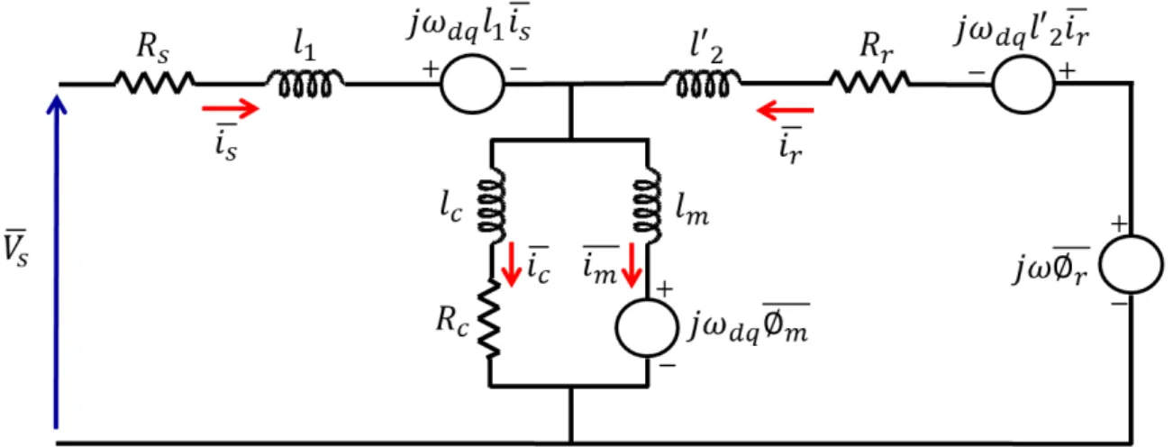
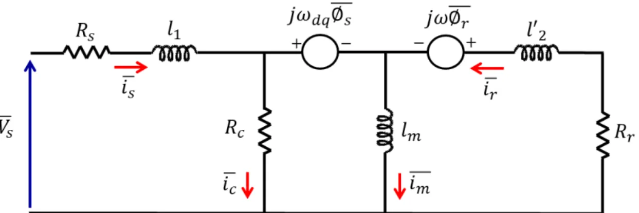
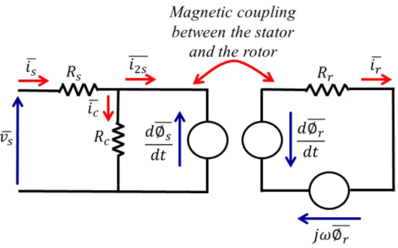
Furthermore, magnetic losses are an important factor which affects the motor performances and the power balance, so that they should be taken into account in the IM dynamic model. Therefore, based on the steady state representation of the core losses equivalent resistor, such types of dynamic models are established in literature, either by using an equivalent resistor and an eddy currents inductance [22] as shown in Fig. 1.4, or by only including the resistor as shown in Fig. 1.5 and detailed in [23] and [24]. The use of the eddy currents inductance increases the accuracy of the magnetic core losses estimation, compared to the constant resistor approach, yet with an increase in the model complexity.
Fig. 1.4. Dynamic model representation including core losses through equivalent resistor and inductance
Several representations and models of the IM are found in literature, with slight differences according to the approach of each study, yet the results are similar and
Chapter 1. Context of the thesis
14
experimentally valid. The main weakness of these two methods lies however in the value of the equivalent resistor which is a constant computed through a series of experiments. Indeed, it is well known that the magnetic laws are affected by many factors, consequently the equivalent resistor representing the core losses in the IM should be a variable element of the circuit, according to the operating point of the motor. This approach would include the effect of eddy currents and other sources of magnetic losses, without having to include an equivalent inductance and increase the model complexity. This method is developed in this work.
Fig. 1.5. d-q dynamic model representation including core losses through equivalent resistor
In order to carry an efficiency study and improve the dynamic model of the IM, it is essential that the loss models be known to be included in the optimization study, especially the core loss model.
1.3 Models of the Main Losses
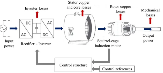
The accurate estimation of the losses in an inverter-fed IM system, shown in Fig. 1.6, is an essential step towards the optimization of its energy efficiency. In this section, the main losses of this system are detailed to be used in a further study in the dynamic model of the IM and in the efficiency optimization process. The motor losses are the copper and mechanical losses already included in the classic dynamic model, in addition to the core losses to be taken into account. The inverter losses are also analyzed to study the effect of the optimization process on all the system losses.
Chapter 1. Context of the thesis
15
Fig. 1.6. Losses in an inverter fed squirrel-cage induction motor system
1.3.1 Copper Losses
The well-known copper losses are the power losses in the system through overheat of the electrical circuit, and are represented by resistors. In the studied system, these losses are due to the stator and rotor resistors and of the motor which appear in the dynamic model of the latter. The Concordia transform used to calculate the alpha-beta currents components ensures power preservation, consequently the global copper losses are written as the sum of the stator losses � in (1.23), and the rotor losses � in (1.24).
� = + (1.23)
� = + (1.24)
1.3.2 Mechanical Losses
The mechanical losses are the friction losses due to the motor bearings, and the aerodynamic losses. They are affected by the rotation speed, as well as by the elements coupled on the motor axis which increase the friction.
These losses are computed as shown in (1.25) using the viscous friction coefficient
Chapter 1. Context of the thesis
16
= �� + � � = �� + |�| (1.25)
1.3.3 Core Losses
The estimation of core losses is an important research domain because of the complexity of magnetic laws and the sensibility of the magnetic circuits to the operating conditions and to the type of material [25]. Thus, they are evaluated in many studies by simply deducting the other known losses and output power, from the input power. In other cases, they are represented by an equivalent resistor in the circuit, and the losses values are computed using the current in this resistor, similarly to the copper losses [58]. Some authors went further by using more specific models, defining these losses as functions of the frequency , and the magnetic field [26]-[55] or flux ∅ [18], as shown in (1.26) and (1.27), where , and are specific coefficients computed through tests.
= (1.26)
= ∅ + ∅ (1.27)
In a more accurate approach, core losses are estimated, according to the Bertotti law [27]-[29], as the sum of the magnetic losses due to the hysteresis effect �, the Eddy currents effect
and the excess losses � caused by the imperfections inside the magnetic circuit. These
losses are written [30] as functions of the maximum value of the magnetic field � and the
voltage frequency as shown in (1.28).
= �+ + �= ′� � + ′ � + ′ � .5� .5 (1.28)
This model contains similarities with the previously presented models, yet in a more detailed and precise approach considering the magnetic characteristics of the analyzed circuit. This model is used in the present study for core losses computation.
The coefficients of the three magnetic losses ′�, ′ and ′ � are not provided by the
motor constructor, their values are measured through a series of experiments [31]. Furthermore, the presented model is only valid for sinusoidal-fed magnetic circuits, and in the inverter-fed case, the effect of the magnetic field harmonics should be taken into account [32]. Thus, as detailed in [33]-[36], the model becomes as shown in (1.29).
Chapter 1. Context of the thesis
17
= ′� � + ′ ∫| |̇ + ′ � .5∫| |̇ .5 (1.29)
Authors have established some simpler versions of the core losses model for non-sinusoidal cases without altering the results [37]. Indeed, by applying the Fourier series, the model becomes as shown in (1.30), where represents the harmonic rank [38].
= ′� � + ′ ∑ �
�
+ ′ � .5∑ .5 �.5
� (1.30)
The core losses model is slightly complicated to use but gives accurate results in sinusoidal and inverter-fed systems while taking into consideration the effect of the geometry of the magnetic structure through the coefficients, as well as the effect of the magnetic field and the frequency.
In order to use the core loss model with measurable variables, the magnetic field is replaced by the product of the flux / and a coefficient characteristic of the magnetic circuit. For instance, equation (1.28) becomes as in (1.31) with the new core loss coefficients
�, and �, products of ′�, ′ and ′ � by . Similarly, equation (1.30) becomes as in
(1.32). = � �+ � + � .5� (1.31) = � �+ ∑ � � + � ∑ .5 �.5 � (1.32)
These losses are a main point in this study, since as mentioned in 1.2, they must be taken into account in the dynamic model of the IM using an accurate loss model, considering the effect of the magnetic field and the frequency, which is ensured by the Bertotti model.
1.3.4 Inverter Losses
In the inverter-motor system, in addition to the motor losses, it is essential to evaluate the losses inside the inverter which are mainly affected by the currents flowing through the phases and switches. These losses are divided into two main parts: the conduction losses caused
Chapter 1. Context of the thesis
18
by the voltage drop in the switches at on-state, and the switching losses due to the switching delay of the elements.
The computation of these losses is not an easy task because of the high switching frequency. In general, the losses at steady-state are averaged over one or multiple switching periods. However, in the case of online calculations or simulations as presented in [39] and [40], and in order to increase accuracy, the conduction losses are instantaneously computed according to the on/off state of the elements, and the switching losses are averaged over a switching period.
1.3.4.1 Conduction Losses
An inverter leg is formed by two switches in series, each one in parallel with an inverted diode. Both switches work in opposite states to avoid short-circuiting the voltage source, and the diodes states are imposed by the sign of the current. The conduction losses depend on the passing element, so it is essential to identify the latter at each state. A series of switching functions is therefore defined to calculate the voltage drop in the switches:
• The function defines the state of the first switch in the studied inverter leg. It is equal to zero for off-state, which corresponds to the on-state of the second switch of the same leg, and to 1 for the on-state,
• The function = − takes the values 1 for on and -1 for off-state,
• The function = + � � . which values vary with the sign of the motor stator current flowing through the switches, in order to identify the element in passing state. The voltage drops according to the state of the switches and to the sign of the flowing current are shown in Table 1.1, where � represents the passing state voltage drop of a switch, and the passing state voltage drop of a diode.
Table 1.1. Conduction voltage drops per inverter leg
= = −
� > �
Chapter 1. Context of the thesis
19
The conduction voltage drop shown in Table 1.1 in each inverter leg is also given by an analytical equation, according to the state of the switches, and the sign of the current, as shown in (1.33).
= . [ �+ − ] (1.33)
The voltage drop values � and of the elements are obtained by the linear equations
(1.34) based on the switches zero-current voltage drop � and and passing resistors � and given by the manufacturer.
{ � == � ++ � (1.34)
Consequently, the inverter conduction losses can be written as in (1.35), where varies according to the state of the switch and the sign of the current as described earlier. Thus, by integrating the loss model over a switching period, would be equal to the duty cycle if the current was positive, and equal to − otherwise. The integrated conduction model is therefore obtained as shown in (1.36).
= | |. [ � + � + − + ] (1.35)
{ > : = . [ � + � + − + ]
< : = − . [ − � + � + + ]
(1.36)
1.3.4.2 Switching Losses
Since the commutations of the switches happen at constant frequency, their losses are averaged [41]-[42]. Indeed, 4 commutations occur in each inverter leg over a switching period, and the on/off delays are provided by the manufacturer. Through these delays, the voltage in the switches is averaged to half the DC bus voltage , and then the switching losses voltage drop is computed as in (1.37), and the conduction losses as in (1.38).
Chapter 1. Context of the thesis
20
= ( + ) | | (1.38)
Based on the above, the global inverter voltage drop can be computed through (1.33) and (1.37), and the global inverter losses in each leg through (1.36) and (1.38). These losses vary with the currents, but depend much on the switches structure because of the passing resistors and switching delays. Generally, silicon-based (Si) IGBT are used, but recently, new Silicon-Carbide (SiC) structures are being manufactured, and ensure better performances in terms of higher switching frequencies, high temperature operation, and most importantly, average reductions of 40% power loss compared to the Si structures. These reductions are due to their smaller semi-conductor structure leading to reduced passing resistors and the capacity to increase the switching frequency and reduce the switching delays.
1.3.5 Summary
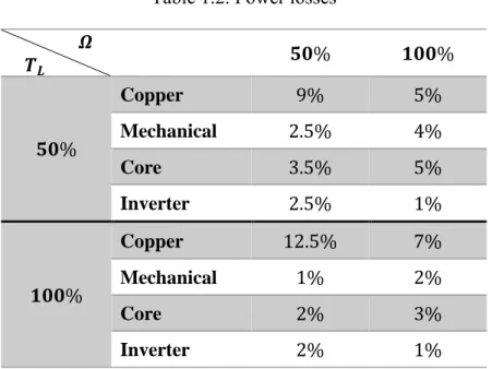
To sum up, the main losses in the inverter-fed IM system are the copper, core and mechanical losses in the motor, in addition to the inverter losses. They vary according to the operating point and power requirements, and can have significant values compared to the input power. Table 1.2 presents results on a 5.5kW IE2 IM, showing percentages of the main losses compared to the system input power at different operating points in the torque-speed plane. Values show that copper losses are the most important ones, and that core losses are also significant, especially at low torque.
It should be noted that the losses depend on different operating variables, so that any optimization process should preserve a balance between them, since the decrease of some variables would increase others. Indeed, the described losses are dependent as follow:
• Copper losses depend on the currents, • Mechanical losses depend on the speed,
• Core losses depend on the voltage and frequency,
Chapter 1. Context of the thesis
21
Table 1.2. Power losses � �� % % % Copper % % Mechanical . % % Core . % % Inverter . % % % Copper . % % Mechanical % % Core % % Inverter % %
According to the above, currents affect copper and inverter losses, and voltage and frequency, or flux, affect core losses. Yet, in order to maintain the load torque requirement, as detailed in 1.2.2, a decrease in flux causes the increase in currents. Consequently, it is essential to keep the best balance between the losses, to reach the optimal operating point. This is addressed in this study, and some optimization techniques are developed in literature for this purpose.
1.4 Energy Efficiency Optimization of the Induction Motor
Several control structures aiming to improve the energy efficiency of the squirrel-cage induction motor are discussed in literature. These methods adapt the flux in the motor according to the operating conditions to reach the best efficiency point [43], since the flux is the only controllable variable in this type of motors. The proposed techniques differ however in the way of reaching the objective [44], some use special algorithms or curves, while others are based on loss models. These methods are presented in this section to introduce the proposed technique of the thesis.
Chapter 1. Context of the thesis
22 1.4.1 Search Control
The Search Control (SC) is an efficiency optimization technique which tracks the lowest possible input power of the motor for each operating point. The input power value is continuously measured and compared to its previous state. The algorithm then decides, whether to keep on varying the flux like its previous state if the input power decreases, or in the other way if the power increases [45]-[47]. By doing so, the system converges to the best efficiency point which corresponds to the minimal input power while keeping on the same output power of the motor. However, an average delay of one second is introduced by each increment/decrement of flux in the basic SC, which causes a global delay of 15 to 20 seconds to reach the optimal operating point. In addition, the control will keep on oscillating around the optimal flux value when in steady state, causing instability of the whole electrical and mechanical system.
Therefore, some other versions of the basic SC are established in literature aiming to improve its performance and reduce the delays to reach the steady-state. For instance, the ‘Golden section’ technique [48] is proposed in literature. It varies the flux increment on the basis of these golden sections theory, in order to find the best efficiency point in a reduced delay. Similarly, artificial intelligence is used in several works [49]-[53] to enhance the search process through training a fuzzy logic controller according to power v/s flux or efficiency v/s flux curves, in order to reach the optimal operating point with reduced delays. Fig. 1.7 shows an example of the improvement in optimal flux tracking between the basic SC and the one with an intelligent controller simulated under MATLAB/Simulink. Delays are clearly reduced, as well as oscillations at steady state. Simulations and experimental tests on the SC techniques validate the improvement in motor efficiency and the decrease in the motor losses.
The advantage of these search control techniques is that they are independent of the motor type or rated power, and do not require any previous knowledge of the system parameters. However, the above detailed problems yet remain significant in terms of delays and oscillations, even if reduced by the enhancement techniques proposed, which could cause the algorithm divergence in cases of rapid load variation or amplified noise in the measured signals.
Chapter 1. Context of the thesis
23
Fig. 1.7. Comparison between SC and intelligent SC flux reference
1.4.2 Loss Minimization Control
Another optimization approach is the loss minimization control (LMC) [18], which computes the flux value corresponding to the minimum losses. Copper and mechanical power losses are estimated through models similar to those detailed in 1.3, as for the core losses, they are either neglected, or estimated using an approximate model. The global losses derivative function is then computed and its zeros give the required optimal flux [54]-[57]. This flux value is then applied through the control to the induction motor.
This technique can be used in several applications, as for example it was developed for electric vehicles[58]-[59], some works proposed enhancements to improve its performance in transient phases with variable load torque [60]-[62], and others proposed hybrid controllers using SC and LMC [63]-[64] to join the advantages of both structures. Results show that the LMC optimization algorithm increases the efficiency especially in the cases of reduced load torques. However, due to the approximate estimation of the core losses, or their omission because of the calculation complexity they cause, the obtained value of optimal flux is not always the most accurate possible. The problem occurs especially at low loads i.e. low currents where the effect of core losses becomes more significant compared to copper losses, and therefore cannot be neglected.
Chapter 1. Context of the thesis
24 1.4.3 Maximum Torque per Ampere
The best efficiency point tracking is also done through the Maximum Torque Per Ampere (MTPA) algorithm [65]-[69], which is also known as Minimum Current Per Torque (MinCPT). It is based on curves computed for a given IM and giving the minimal value of current per torque as shown in Fig. 1.8, the corresponding flux is then applied to the motor through the control structure. Similar works as in [70]-[72] take into account the magnetic saturation effect to obtain more accurate values of flux according to the operating point. Other works like in [73] combine the MTPA strategy and the intelligent SC in a hybrid controller to join the advantages of both structures.
Simulation and experimental results show efficiency increase and losses decrease using the MTPA. However, the efficiency optimization through this method is not always guaranteed to give the best results because of the effect of core losses. Indeed, the latter are known to increase while copper losses decrease because of the opposite variations of flux and currents in the motor. Therefore, the best currents value does not necessarily correspond to the best efficiency point, and consequently, in order to obtain the most accurate value of optimal flux, the effect of core losses should also be taken into account in the study.
Chapter 1. Context of the thesis
25 1.4.4 Summary
The improvement methods found in literature are proven to optimize the energy efficiency of induction motors and reduce their losses. Yet, each one of the methods has weaknesses either in terms of dynamic response in the case of SC, or in terms of optimal efficiency accuracy in the case of LMC and MTPA. Core losses constitute an important aspect of efficiency estimation; therefore, it cannot be omitted or taken into consideration through an approximate approach.
The proposed method in this study tracks the best efficiency point avoiding the dynamic delays and oscillations, and taking the core losses into consideration the most accurately possible. The technique is based on off-line measurements to accurately map the optimal reference flux in the torque-speed plane. The approach is systematic and can be declined very quickly on any asynchronous machine.
Conclusion
This work is well positioned in the heart of the European Commission sustainability project, by contributing in the efficiency optimization objective. For this purpose, models of the squirrel-cage induction motor were presented in this chapter, as well as loss models aiming to analyze the optimization effect on the main losses in the IM and in the inverter. Hence, several techniques found in the literature serving that goal are presented. However, these methods lack accuracy in some cases and can be subject to dynamic instabilities.
Through the present study, an improved optimization method is proposed, avoiding the problems of the existing techniques, and based on an improved dynamic model of the induction motor which is to be presented in the next chapter. This model takes into account the effect of the core losses, in addition to the other motor losses which are included in the classic model version. The goal is to find the flux corresponding to the optimal balance between the system losses, and include it into the control structures afterward.
Chapter 2 Induction Motor Model Taking Core Losses into
Account
Table of Contents
Introduction ... 27 2.1 Model Parameters Measurement ... 27 2.1.1 Mechanical Parameters ... 27 2.1.2 Electrical Parameters ... 28 2.1.3 Core Losses Model Coefficients ... 30 2.2 Including Core Losses in the IM Model ... 31 2.2.1 Equivalent Torque Approach... 32 2.2.2 Equivalent Resistor Approach ... 32 2.2.3 Summary and Analysis ... 34 2.3 Including Variable Core Losses ... 37 2.3.1 Enhancement of the Improved Dynamic Model ... 38 2.3.2 Simulation Results and Experimental Validation ... 38 Conclusion ... 39
Chapter 2. Induction Motor Model Taking Core Losses into Account
27
Introduction
Establishing an accurate mathematical model is an essential step for any study to be carried on a motor, as it allows a precise simulation of the performance to be expected under specific conditions. The classic model of an IM lacks accuracy because it neglects the effect of core losses.
In this chapter, an improved model taking into account such losses is thus proposed. This model is based on the addition of a variable resistor representing core losses which depend on the magnetic field and frequency. It is calculated using the Bertotti model presented in 1.3.3. In addition, the experimental measurement and identification of motor parameters are detailed, especially for the core losses parameters to be used in the proposed model. The variation of these losses with the operating conditions is also taken into account.
2.1 Model Parameters Measurement
The studied motor is a 5.5kW Leroy-Somer squirrel-cage induction motor LSES 132 SU compliant with IE2 efficiency standard. The parameters of the studied motor are computed through a series of experiments carried in several operating conditions. The obtained parameters define the classic dynamic model of the IM detailed in 1.2.2, as well as the core losses model presented in 1.3.3.
2.1.1 Mechanical Parameters
The mechanical parameters of the IM that need to be measured are the viscous friction coefficient � and the dry friction torque that define the friction losses on the axe of the
motor, and take part in the mechanical equation of the IM dynamic model. They are computed through a zero-load deceleration experiment, where the IM initially rotating slightly below the base speed is powered off. The speed is measured and is presented in Fig. 2.1.