HAL Id: hal-01823752
https://hal-amu.archives-ouvertes.fr/hal-01823752
Submitted on 26 Jun 2018
HAL is a multi-disciplinary open access
archive for the deposit and dissemination of
sci-entific research documents, whether they are
pub-lished or not. The documents may come from
teaching and research institutions in France or
abroad, or from public or private research centers.
L’archive ouverte pluridisciplinaire HAL, est
destinée au dépôt et à la diffusion de documents
scientifiques de niveau recherche, publiés ou non,
émanant des établissements d’enseignement et de
recherche français ou étrangers, des laboratoires
publics ou privés.
An Iterative Method Using Conditional Second-Order
Statistics Applied to the Blind Source Separation
Problem
Bernard Xerri, Bruno Borloz
To cite this version:
Bernard Xerri, Bruno Borloz. An Iterative Method Using Conditional Second-Order Statistics Applied
to the Blind Source Separation Problem. IEEE Transactions on Signal Processing, Institute of
Electri-cal and Electronics Engineers, 2004, 52 (2), pp.313-328. �10.1109/TSP.2003.820986�. �hal-01823752�
An Iterative Method Using Conditional
Second-Order Statistics Applied to the Blind
Source Separation Problem
Bernard Xerri - Bruno Borloz
SIS/GESSY - ISITV
Universit´e de Toulon et du Var
Av. Georges Pompidou, BP 56
83162 LA VALETTE DU VAR CEDEX (FRANCE)
xerri,[email protected]
Abstract
This paper is concerned with the problem of blind separation of instantaneous mixture of sources (BSS) which has been addressed in many ways. When power spectral densities of the sources are different, methods using second-order statistics are sufficient to solve this problem. Otherwise these methods fail and others (higher-order statistics,...) must be used.
In this paper, we propose an iterative method to process the case of sources with the same power spectral density. This method is based on an evaluation of conditional first and second-order statistics only. Restrictions on characteristics of sources are given to reach a solution, and proofs of convergence of the algorithm are provided for particular cases of probability density functions. Robustness of this algorithm with respect to the number of sources is shown through computer simulations. A particular case of sources which have a probability density function with unbounded domain of definition is described; here the algorithm does not lead directly to a separation state, but to an a priori known mixture state. Finally, prospects of links with contrast functions are mentioned, with a possible generalization of them based on results obtained with particular sources.
Keywords
KEY WORDS : blind source separation; conditional statistics; iterative method; performance index; contrast functions
I. Introduction
Blind source separation problem is currently receiving an increased interest [14][6][17][9][22] in numerous engineering applications. This problem consists in restoring N unknown, statistically independent random sources from N available observations which are linear combinations of these sources.
Methods based on second-order statistics (AMUSE [28], SOBI [4] or IMISO [10]) have been extensively used to solve BSS problem. These methods perform well when power spectral densities (PSD) of sources are different. Otherwise High-Order Statistics (HOS) methods are required [19][29][8][23][31], subjected to delicate estimation: for example iterative methods using fourth-order cumulants have been early studied [7].
In this paper, we present a new iterative method based on the evaluation of only first and second-order statistics estimated from extracted series of observations (we talk of conditional statistics), avoiding calculation of high-order quantities. The main advantage of this method is that, like usual HOS techniques, it allows to process certain cases where PSD’s of sources are the same; hence, it can doubtless be interpreted as an HOS method. However, in this paper, we deliberately do not compare HOS methods to ours from the theoretical point of view: for example, we do not approach the theoretical problems of robustness with respect to the number of sources. But numerical comparisons with a classical HOS method (JADE) are provided in this paper to draw conditions for which our method brings an improvement.
Indeed this method is sensitive to probability density functions (PDF) of sources, and conditions on these PDF’s are necessary to reach separation: these conditions are not very restrictive and usual domains of application as digital communications, etc... respect them. We will see that this method restores sources of same or different PSD’s as well. We prove that our method converges. Classically HOS methods use contrast functions and impose a convergence to a separation state [20][27][24]. We will prove that our method converges to a state which can be known according to PDF’s of sources (then of engineering
applications), and which is not necessarily a separation state: this method cannot be linked to a contrast function but nevertheless yields the separation. Some particular types of PDF’s are more detailed.
To solve BSS problem for an instantaneous mixture, there exist different methods: HOS methods (algorithm JADE for example), geometrical methods [2][25][26] or neural network methods [3][15]. Severe restrictive conditions must be verified for geometrical methods to work: PDF’s of sources must have a bounded domain of definition and results are very sensible to the density on the edges.
Some authors use the property of non-stationarity of signals (for example: speech signals) to solve BSS problem: in the case of instantaneous mixtures [33] or of convolutive mixtures [32]: this assumption of non-stationarity is crucial for their algorithms. For instance, this assumption allows [33] to use only second-order moments and an iterative procedure.
Concerning the present paper, in the mind of authors, the main idea of the method proposed is that it uses conditional statistics (restricted up to second-order ones) through an iterative algorithm. We are aware that HOS are efficient to solve the BSS problem for the instantaneous mixture model provided that cumulants are not null (non-gaussian signals). We are also aware that the convolutive mixture model is presently the main field of researches for the BSS problem, and that a method which works for instantaneous mixture could seem to bring little. However, as far as we know, it appears to us that the approach proposed is original enough; in a first time, this method needed to be tried and justified within the framework of the more simple model of instantaneous mixture; proofs are already not obvious to bring in this more simple model. Adaptation of this method for the more general convolutive mixtures model (reverberations for example) will be treated in a forthcoming paper. Hence, in a first step, this paper restrains deliberately its topic to the instantaneous mixture model for which proofs can be provided.
Formulation of the problem
For blind source separation problem, we consider N unknown and statistically independent sources X, and N available observations Y = M X where M is an unknown deterministic nonsingular constant matrix called mixture matrix. The BSS problem consists in restoring sources X by applying to Y an unknown linear transformation S, so that SM = ΛΠ: this is a product of a nonsingular diagonal matrix and a permutation matrix. Thus S is a separating matrix. The algorithm proposed calculates at each step a matrix Ki so that the resulting matrix KnKn−1...K1 associated with the a priori knowledge of the state
at the end of convergence tends to a separating matrix when n increases.
Organization of the paper
This paper is organized as follows. Section II formulates the mathematical model and introduces tools for study. Section III summarizes a few classical methods using only second order moments and underlines their limitations; the aim of the method proposed is to reduce them. After a detailed presentation of the reasons which lead us to the method proposed in section IV, our algorithm is explained in section V; its limitations and methods used to quantify its performances are described. Section VI is dedicated to analysis of convergence of this algorithm. Calculation of conditional moments in different interesting
cases is done. Proof of convergence of the algorithm is given according to PDF’s of sources. Monte-Carlo simulation results are presented in section VII; robustness of this algorithm with respect to the number of sources is illustrated for some specific cases.
II. Basic assumptions and problem formulation
A. Basic assumptions
Let us consider N zero-mean random sources assumed to be unknown, stationary and statistically independent: X(t) = ³ X1(t) ... XN(t) ´T .
Through a set of receivers, N observations are available:
Y (t) =³Y1(t) ... YN(t)
´T
,
which are linearly linked to sources by:
Y (t) = M X(t), (1) where M is an unknown deterministic nonsingular constant matrix called mixture matrix. This relation can also be written:
Yi(t) = N
X
j=1
αijXj(t) ∀i = 1, ..., N.
We will note RY(τ ) the spatial covariance matrix of Y (t) for a lag τ : RY(τ ) , E
¡ Y (t)YT(t + τ )¢. By assumption, RX(τ ) , E ¡ X(t)XT(t + τ )¢is a diagonal matrix. B. Problem formulation
The principle of separation, i.e. restoration of sources, consists in applying a linear transformation S to Y to generate N signals zi statistically independent and proportional to sources xi:
Z , SY = SM X.
There are two inherent indeterminacies concerning the order i and the power σ2
i of each source. Hence,
the matrix S is valid if it verifies:
SM = ΛΠ
with Λ nonsingular diagonal matrix and Π permutation matrix. Furthermore, the indeterminacy concern-ing σ2
i allows, without loss of generality, to consider σ2i = 1; thus the spatial covariance matrix of sources
at lag 0 is
RX(0) = E
¡
X(t)XT(t)¢= I N
C. Measure index of closeness to ΛΠ
For the needs of our algorithm, we have to define an index which measures the closeness of a matrix A to ΛΠ. To quantify such a proximity, we will use an adapted version of the performance index proposed by E. Moreau [20]; this one, which indicates how a matrix A is close to ΛΠ, is noted ind0(M ) and is
defined as follows: ind0(A) , 1 2N (N − 1) XN i=1 XN j=1 |aij|2 max k |aik| 2 − 1 + · · · · · · N X j=1 N X i=1 |aij|2 max k |akj| 2 − 1 ,
and has the following properties: ¦ 0 6 ind0(A) 6 1
¦ ind0(A) = ind0(ΠA)
¦ ind0(A) = 0 ⇔ A = ΛΠ
¦ if α is a nonzero scalar, ind0(αA) = ind0(A)
Notwithstanding its properties, this performance index does not suit for our needs. We want an index
ind(.) which verifies also the additional property: ind (ΛA) = ind (A). A way to complete this requirement
is to apply to A the following transformation:
A = [aij]−→ u(A) =u a11 δ1 · · · a1N δ1 .. . · · · ... aN 1 δN · · · aN N δN with δi= p a2
i1+ ... + a2iN, and then to apply the classical performance index to u(A) in lieu of A:
ind(A) , ind0(u(A)).
Note first that if U is a unitary matrix, u(U ) = U and then ind(U ) = ind0(U ), and secondly that
a normalization of rows of A by δi = max
j (aij) would be effective as well. From here, we will call
’performance index of A’ the value ind(A).
III. Classical second order methods
Methods using second-order statistics have been successfully proposed by several authors for the case of sources with different PSD’s. Some of them are presented hereafter.
A. AMUSE
The AMUSE (Algorithm for Multiple Unknown Signals Extraction) algorithm proposed by L. Tong and al. [28] processes the more general following model:
where n(t) is a corrupting noise.
This algorithm computes an SVD of the spatial covariance RY(0) = E
¡
Y (t)YT(t)¢and estimates the
number of sources from the number of significant singular values and noise variance from others. Then it performs an orthogonalization transformation W applied to Y (t): Yw(t) , W Y (t). A judicious choice of
a lag τ such that RYw(τ ) has distinct eigenvalues, leads to signal estimation ˆX(t) = UTW Y (t) where U
is the corresponding eigenmatrix.
B. SOBI
The SOBI (Second Order Blind Identification) algorithm has been proposed by A. Belouchrani and al. [4].
A matrix W can be found to ensure spatial decorrelation of the process Yw(t) , W Y (t). For a lag
τ 6= 0, the covariance matrix of whitened observations Yw(t) is RYw(τ ) , W RY(τ )W
T which can be
written RYw(τ ) = W M RX(τ )MTWT = U RX(τ )UT, where U is a unitary matrix to be evaluated.
Matrices RX(τ ) are diagonal and then U is the eigenmatrix for all matrices RY(τ ), ∀τ . If a value τp of τ
for which RY(τp) has distinct eigenvalues can be found, U can be completely determined. An interesting
option is to choose a set of values of τ say {τ1, ..., τk} and to perform a simultaneous diagonalization
of the set of matrices [RYw(τ1), RYw(τ2), ..., RYw(τk)]. This technique which has been introduced in [5],
consists in a generalization of Jacobi’s method to diagonalize an hermitian matrix. Knowing U , sources are restored by ˆX(t) = UTW Y (t).
C. IMISO
The IMISO (Identification de M´elanges Instantan´es au Second Ordre – Second Order Identification of Instantaneous Mixtures) algorithm proposed by J.F. Cavassilas and al. [10][13] is a natural extension of previous one and can be summarized as follows: the covariance matrix of observations is
RY(τ ) = M RX(τ )MT.
For commonly encountered signals (band-limited), it is reasonable to postulate that RY(τ ) is indefinitely
differentiable with respect to τ . Then
R(2k)Y (0)M−T = RY(0)M−TRX−1(0)R
(2k)
X (0).
This is a generalized eigen-problem:
RY(0)V = R(2k)Y (0)V D,
where D = R−1X (0)RX(2k)(0) is obviously a diagonal matrix, and V = M−T (except for a diagonal and a
permutation matrix). Then, applying VT = M−1to Y leads to X (except for a diagonal and a permutation
matrix).
¦ R(2k)Y (0) and RY(0) must be symmetric and one out of them must be positive definite; this condition
is always guaranteed.
¦ no row of R(2k)Y (0) must be proportional to a row of RY(0); such a thing would correspond to the
case where second-order series expansion of normalized autocorrelation functions of sources are identical or very close in vicinity of 0; this assumption is generally not realistic. This case is involved if R−1Y (0)R(2k)Y (0) has a multiple eigenvalue, i.e. there is an indeterminacy within the eigen-subspace concerning the choice of eigenvectors to take into account. If PSD’s (therefore autocorrelation functions) of sources are identical, there is one eigenvalue of multiplicity N : indeterminacy is complete: it is not possible to extract privileged directions.
Experimentally a value k=1 (second order derivative) is then often sufficient, but a value k=2 (or more) may be necessary to solve the problem.
A generalized method, including AMUSE and IMISO as particular cases, has been recently proposed by J. Barr`ere and G. Chabriel [1].
D. Limitations of these methods
There is unfortunately a severe limitation to these methods: they work in one step only with second-order statistics. This is why it is not possible to use them to restore sources which have the same PSD: sources must be differently colored. In such a case, people usually try to solve the problem by using higher-order statistics: the main disadvantage of such an approach lies in the estimation of higher-order moments which becomes quickly difficult when N increases.
For sources with identical PSD, the way of using first and second-order conditional statistics through an iterative formulation seems attractive. Nevertheless, the idea remains to find a linear transformation that makes independent observations.
IV. Use of conditional statistics
A. Introduction
The idea of previous algorithms is always to find two functions of Y = M X, f1 and f2 verifying the
property of linearity
fi(Y ) = M fi(X) ∀i
and such as the two matrices
Ri = E ¡ fi(Y )fiT(Y ) ¢ = M E¡fi(X)fiT(X) ¢ MT = M D iMT verify that R−1 1 R2= M−TD−11 D2MT, (2)
is an eigenvalue problem (this is the case provided that D−1
1 D2 is a diagonal matrix) with non-multiple
and a permutation matrix). In the case of identical PSD, there is a unique eigenvalue of multiplicity N , and this approach (classical second-order moments) is hopeless.
B. Conditional statistics
Let us introduce conditional moments. Our problem is very specific since practically only linear com-binations of sources are available (1), say the observations Yi. For example, the condition used can be:
Yi> 0.
Conditional first and second-order moments are E (Y /Yi> 0) and E
¡
Y YT/Y i> 0
¢
. The second one is naturally one out of the two matrices needed, say R1. Denoting ν , E(Y /Yi> 0), it is tempting to define
R2= E ¡ (Y − ν)(Y − ν)T/Y i> 0 ¢ . Then R−11 R2= R−11 (R1− ννT) = IN − R−11 ννT.
Noting conditional mean of sources (N -dimension vector)
µ = E (X/Yi> 0) , (3)
and conditional covariance matrix of sources
D = E¡XXT/Y i> 0 ¢ , (4) it comes R−11 R2= M−T ¡ IN − D−1µµT ¢ MT.
Generally IN− D−1µµT is not a diagonal matrix. However, this must be the case if separation is already
reached: Y = X (M = IN). In such a case, µ is a vector whose all components are null except the ith
which is strictly positive. The term µµT is already a diagonal matrix (with only one non-zero term).
Matrix D remains to be studied.
If we note Di the domain of definition of source Xi, the hyper-volume described by all sources is then
Σ = D1× ... × DN ⊂ RN. Let us consider one observation Yi =
PN
k=1αikXk. The equation ”Yi = 0” is
those of an hyperplane Π passing through O; Π divides Σ into two parts Σi (Yi=
PN
k=1αikXk> 0) and
Σ0
i (Yi< 0). Using condition ”Yi> 0” describes the hyper-volume Σi.
Making appear the joint conditional PDF of X under the condition Yi > 0: pX/Yi>0(x1, ..., xN), it
comes that the jthcomponent of µ is given by:
µj =
Z
RN
xjpX/Yi>0(x1, ..., xN)dx1...dxN,
and element of row j and column k of D is
Djk=
Z
RN
Like in the case of expected values under a discrete random variable condition, we can calculate these expressions as following: noting P (Yi> 0) =
R
ΣipX(x1, ..., xN)dx1...dxN the probability that the ith
observation is positive, they are both calculated by integrating first or second-order moments in Σi:
µj = 1 P (Yi> 0) Z Σi xjpX(x1, ..., xN)dx1...dxN, (5) and Djk= 1 P (Yi> 0) Z Σi xjxkpX(x1, ..., xN)dx1...dxN. (6)
Of course as sources are independent, pX(x1, ..., xN) = p1(x1)...pN(xN).
D is not diagonal in the general case. However, as the condition used is linear passing through O, it
can be proved that if PDF’s of sources are symmetrical (xi ∈ Di ⇒ −xi ∈ Di and pi(xi) = pi(−xi)),
then P (Yi> 0) = 12 and matrix D is diagonal of terms
Djj =
Z
Dj
x2p
j(x)dx = σj2.
We can note that this term does not depend on the hyperplane Π chosen but only on PDF’s of sources. proof
Let us state that the PDF’s pi(x) of sources are symmetrical. Σi and Σ0i are symmetrical: effectively,
x = (x1, x2, ...xN) ∈ Σi⇒ −x = (−x1, −x2, ... − xN) ∈ Σ0i. (7)
Then defining fnm
ij (x) = xnixmj p1(x1)...pN(xN), which verifies the property
fnm ij (−x) = (−1)n+mfijnm(x) ∀x ∈ Σ, (8) Z Σ fnm ij (x)dx = Z Σi fnm ij (x)dx + Z Σ0 i fnm ij (x)dx + Z Π fnm ij (x)dx. fnm
ij (x) being a continuous function with ’good properties’, the last term is null, and
Z Σ fnm ij (x)dx = Z Σi fnm ij (x)dx + Z Σ0 i fnm ij (x)dx.
Furthermore, from (7) and (8), Z Σ0 i fijnm(x)dx = (−1)n+m Z Σi fijnm(x)dx. If n + m is even Z Σi fijnm(x)dx = 1 2 Z Σ fijnm(x)dx = 1 2E(X n iXjm).
This term depends no more on the condition chosen but only on PDF’s of Xi and Xj.
As Xi and Xj are independent, if i 6= j, this expression becomes 12E(Xin)E(Xjm); in this case, if n or m
is odd, it becomes null. If i = j, then we obtain the (n + m)th-moment of X j.
If n = m = 0 we obtain P (Yi> 0) = 12.
If n = m = 1 we obtain the elements of the matrix D which is diagonal of term Djj = σj2. ¤
C. Conclusion
In conclusion, if we want to respect the condition ”D is a diagonal matrix”, two sufficient (but not necessary) conditions are:
• PDF’s of sources are symmetrical,
• the condition to take into account is the equation of an hyperplane passing through O.
First condition is a very acceptable one: in the field of digital communications, signals are usually uniformly distributed (with a limited or unlimited number of states), ...
The second one is in fact imposed by the problem: available quantities are observations, i.e. linear combinations of sources.
For reasons explained in this section and others that will be detailed later, those both conditions will be stated to be verified in next sections.
V. Presentation of the algorithm
This section is devoted to a general presentation of the algorithm proposed. In the light of previous section, this algorithm relies on an iterative application of an adaptation of the generalized algorithm described in section IV with conditional statistics: a linear condition (based on observations) is used to make appear those conditional statistics.
A. Principle of the algorithm
Let us expose the mechanism to restore sources. As said in previous section, we first extract from ob-servations a conditional subsequence of them, called conditional obob-servations and noted Yci= (Y /Yi> 0),
or: Yci = ³ Yci,1 ... Yci,N ´T .
This is a highly nonlinear operation and Yci,i > 0. Obviously E (Yci) = E(Y /Yi > 0) 6= 0, and we can
define ˜Yci , Yci− qci where qci = E (Yci).
From these extracted observations, we calculate the N -by-N covariance matrices of Yci and ˜Yci noted:
Rci , E ¡ YciY T ci ¢ = E¡Y YT/Yi> 0 ¢ and ˜ Rci, E ³ ˜ YciY˜ T ci ´ = Rci− E (Y /Yi> 0) E (Y /Yi> 0) T .
Now let us define
Γci , R
−1 ci R˜ci,
and let us process the eigen-decomposition of Γci:
If we write (1) as Y(1) = M(1)X, denoting the first iteration of our algorithm, and then apply PT to
Y(1) (this is natural according to the comment linked to equation (2) in section IV), we obtain a new
combination of observations called ”new observations”
Y(2)= PTY(1)= PTM(1)X = M(2)X,
which appears as a new mixture of sources; M(2) is the new mixture matrix:
M(2)= PTM(1). (9)
Here, the first step of our algorithm is finished. If properties of M(2) are satisfying, this step can be
iterated again on new observations Y(2).
P is determined except for a permutation and a power. In other words, P ΛΠ (or P ΠΛ) are also
eigen-vectors of Γc1: those both indeterminacies involved in Λ and Π correspond to the inherent indeterminacies
aforementioned regarding power of sources and their order. P can be normalized readily. When applying
PT to observations Y , we apply in fact the transformation ΛΠPT (or ΠΛPT). According to section II-C,
ind(ΛΠPTM(1)) = ind(PTM(1)) = ind(M(2)).
If P is a diagonal matrix, no improvement has been brought by the transformation: this observation leads to determine the criterion to stop convergence.
test for end of convergence As M is unknown, mixture matrix M(n) at step n is never reachable.
Even if we use it for proofs of convergence, we cannot use it practically during convergence to test the closeness of our solution to the good one.
Nevertheless, matrix P being available at each step, we stop iterative process for an ind(P ) smaller than a value ε defined beforehand, i.e. when the transformation matrix P is close to the product ΛΠ, in other words when convergence is achieved.
We will study in section VI the state at the end of convergence.
general methodology of algorithm Y(0)= Y .
Let’s consider modified observations available at step n: Y(n)=³Y(n)
1 ... Y (n)
N
´T
.
1) Create extracted observations Yci = (Y /Yi> 0).
2) Compute zero-mean extracted observations ˜Yci = Yci− E (Yci).
3) Estimate Rci and ˜Rci.
4) Calculate Γci= R
−1 ci R˜ci.
5) Calculate the eigenvectors P of Γci.
6) Apply the transformation PT to Y(n): Y(n+1)= PTY(n)= M(n+1)X.
remark: Γci can also be written Γci = IN − R
−1 ci qciq
T
ci. Eigenvectors of Γci are then R
−1
ci qci (associated
with eigenvalue 1 − qT ciR
−1
ci qci) and N − 1 vectors orthogonal to qci associated with the same eigenvalue
1, say (q⊥ ci,1, ...q ⊥ ci,N −1). Then P = ³ R−1 ci qci qc⊥i,1 ... q ⊥ ci,N −1 ´ .
We note that there is an eigenvalue with multiplicity N −1 which corresponds to a subspace of dimension
N −1 in which there is an indeterminacy for the choice of N −1 eigenvectors (this indeterminacy is cancelled
if N = 2). In fact practically we observe that the algorithm applied stricto sensu extracts one out of the sources. If one source is found, it is theoretically possible to extract it and to reduce the problem to a (N − 1)-dimension problem. Practically however, a significant deterioration appears quickly, and such a way is not conceivable. The way of a simultaneous extraction of all the sources is greatly preferable. The algorithm needs to be modified: as mixture matrix is nonsingular, it is reasonable to suppose that the same test (of series extraction) applied to each observation will lead to N satisfactory vectors, i.e. linearly independent. Consequently the algorithm is modified as follows:
Summarized basic algorithm at step n Y(0)= Y .
Let’s consider modified observations available at step n: Y(n)=³
Y1(n) ... YN(n)
´T
.
1) For i=1 to N ,
1-a) Create extracted observations Yci = (Y /Yi> 0).
1-b) Compute qci , E (Yci). 1-c) Estimate Rci, E ¡ YciY T ci ¢ . 1-d) Calculate pi, R−1ci qci. 2) Create P = ³ R−1 c1 qc1 ... R −1 cNqcN ´ = ³ p1 ... pN ´ .
3) Apply the transformation PT to Y(n): Y(n+1)= PTY(n)= M(n+1)X.
4) If ind(P ) < ε stop iterations. B. Rewriting according to sources
To study properties of the algorithm, let’s see its implications with regard to sources. We will use the same notation for Xci extracted sequence of X corresponding to Yci (such as Yci = M Xci); we will note
µci , E(Xci) = E(X/Yi > 0), ˜Xci , Xci− µci and Dci , E
¡ XciXcTi ¢ = E¡XXT/Y i > 0 ¢ . Obviously, it is not possible to estimate directly these quantities linked to X from available data (i.e. the sole observations) while Γci can be calculated. We deduce that:
Rci = M DciM T, and ˜ Rci = M ¡ Dci− µciµ T ci ¢ MT.
Then Γci = M −T ¡I N − Dc−1i µciµ T ci ¢ MT, which implies ¡ IN − Dc−1i µciµ T ci ¢ MTP = MTP Q.
This expression makes appear MTP which from (9) equals¡M(2)¢T. If we define V = MTP (VT = M(2)),
then V and Q are eigenvectors and eigenvalues of¡IN − Dc−1i µciµ
T ci ¢ : ¡ IN − Dc−1i µciµ T ci ¢ V = V Q. (10)
P and Q depend on Y and are then calculable, while V is not.
From (10) we can assert that the N − 1 linearly independent vectors orthogonal to µci (µ⊥ci,k such as
µT ciµ
⊥
ci,k = 0 ∀ k = 1, ..., N − 1) are also eigenvectors of
¡
IN− D−1ci µciµ
T ci
¢
with the same eigenvalue 1. It is easy to verify that D−1
ci µci is an eigenvector of ¡ IN − D−1ci µciµ T ci ¢
associated with the eigenvalue 1 − µT
ciD
−1
ci µci. Hence, we can write:
VT =³ D−1 ci µci µ ⊥ ci,1 ... µ ⊥ ci,N −1 ´T = M(2).
If we apply the modified algorithm, instead of this expression, new mixture matrix will be
M(2)=³ D−1 c1 µc1 ... D −1 cNµcN ´T . The ithline of M(2) is Mi(2)=¡D−1 ci µci ¢T . (11)
One line of M(2) depends on corresponding line in M(1) and PDF’s of sources. Theoretical expression of
M(2) is known. We will see that the difficulty lies in calculation of µ
ci.
From IV-B, if PDF’s of sources are symmetrical then P (Yi> 0) = 12 and covariance matrix Dci is
diagonal of terms Dci,jj= σ 2 j. (12) In this case Mi(2)= h µci,1 Dci,11 ... µci,N Dci,NN i .
Obviously if PDF’s are identical of power σ2, this matrix becomes scalar: D
ci,jj= σ2, and Mi(2)= 1 σ2 h µci,1 ... µci,N i .
remark: limitations of the study of convergence We readily see that Mi(2) (and therefore M(2))
closely depends on the PDF’s of sources. This is the main limitation of the study of convergence of this algorithm: theoretical calculation of µci and Dci may hardly be done in a general way. Unfortunately
proof of efficiency of the algorithm must be provided for each specific sort of PDF. This observation will prompt us to focus our attention on some noteworthy cases of PDF’s, even if general considerations can be brought.
C. Remark about a whitening stage of observations
Before running the algorithm, it is always possible to whiten observations. Then at each step, the transformation matrix P must comply with these constraint: P must be a unitary matrix. Hence M(2)
is also unitary. This procedure comes down to make orthogonal lines of M(2) calculated by the
al-gorithm. Practically expressions R−1
ci qci are calculated and normalized to 1, then P is calculated by
P = ³R−1
c1 qc1 ... R
−1 cNqcN
´
and forced to be orthogonal by columns. This is only a guarantee not to converge twice or more to the same source for different initial conditions.
Practically the matrix P obtained is indeed nearly but not exactly orthogonal. However, because of this very small distance to a unitary matrix, simulations show that, without imposing a constraint of orthogonality to P at each step, the algorithm derives slowly to a situation where mixture matrix becomes non-invertible, and certain sources are found twice or more while some others are lost. So it becomes necessary to impose such a constraint to P (in practice, vectors (columns) Pi of P are normalized by a
Gram-Schmidt algorithm, and its normalization is never a problem because sources are retrieved except for their power). By constraining P to be orthogonal, the correction brought is not as much important than could appear. This constraint just imposes that two lines of new mixture matrix are orthogonal.
However it is not necessary to pre-whiten observations. When observations Y are whitened, that means that a linear transformation W = √D−1UT is applied to Y where U and D are respectively
the eigenvectors and eigenvalues matrices of covariance matrix E¡Y YT¢. If observations are whitened,
transformation matrix P must comply with some constraints; let’s note Φ = PTW−1. A procedure is
used to make Φ orthogonal. Transformation applied to Y will be ΦW in lieu of PT. This is a manner of
avoiding pre-whitening stage of observations, but keeping the structure of invertible mixture matrix. VI. Analysis of convergence according to PDF
In the light of previous sections, throughout this section we state that sources have symmetric PDF’s.
A. Assumptions and notations
Let us consider one observation Yi=
PN
k=1αikXk, i.e. one line of the mixture matrix M
Mi(1)= h
αi1 ... αiN
i ;
Mi(1) can be considered as a point in RN.
After one step of our algorithm, the new observation Yi(2)corresponds to the ithline of the new mixture
matrix, which from (11) verifies:
Mi(2) = h
mi1 mi2 ... miN
i
= D−1ci µci,
where µci and Dci are given by (3) and (4); their components are respectively calculated by (5) and (6).
mij = µci,j Dci,jj = R Σixjp1(x1)...pN(xN)dx1...dxN R Σix2jp1(x1)...pN(xN)dx1...dxN j = 1, ...N. (13)
As PDF’s of sources are symmetrical, mij = µci,j σ2 j = 2 R Σixjp1(x1)...pN(xN)dx1...dxN σ2 j . (14)
Study consists in comparing the ith line of M(1) and the ith line of M(2). This comparison is made
trough the index performance naturally adapted to one line. A constraint exists nevertheless: M is invertible; at each step this constraint must be verified to ensure coherence of columns of new mixture matrix. If a pre-whitening stage is processed, this constraint is simply: ’P is unitary’.
B. Miscellaneous considerations
From the point of view of the algorithm there is no restriction to normalize Mi(1), e.g. by its largest value: if |αi1| > |αij| ∀j, this line is equivalent to
h 1 αi2 αi1 ... αiN αi1 i
(the hyperplane of equation PN
k=1αikXk = 0 is the same than
PN
k=1ααiki1Xk = 0).
B.1 Fixed-points of the algorithm
We define a fixed-point of the algorithm as a point such as, after one step, the new observation Yi(2) corresponds to the following (normalized) line of new mixture matrix:
h
1 γi2 ... γiN
i
, verifying
∀j = 2, ...N, γij =ααiji1.
We want to study the behavior of our algorithm around its fixed-points. For each fixed-point we want to determine if it is attractive or repulsive.
B.2 Absence of one source in observation
Let us consider the case where one source Xi is not present in observation Y1(i.e. α1i= 0). The initial
mixture line is h α11 ... α1,i−1 0 α1,i+1 ... α1N
i
. Numerator of m1i in equation (13) can than
be written: Z · · · Z N P k=1 k6=i αkxk>0
p1(x1)...pi−1(xi−1)pi+1(xi+1)...pN(xN)dx1...dxi−1dxi+1...dxN ×
+∞
Z
−∞
xipi(xi)dxi.
As sources are zero-mean, this term is null: m1i= 0.
Conclusion As expected a source cannot appear in a line if it is not present from the start. The final line will be necessarily like
h
m11 ... m1,i−1 0 m1,i+1 ... m1N
i .
B.3 Observations of the form Yi= α q
P
k=1
Xk with q ≤ N
Let us find conditions for points like h
α ... α 0 ... 0
i
with q ’α’ and p ’0’ (p + q = N ) to be fixed-points of the algorithm.
The p last sources can take every value in their domain of definition. Numerator of mij in equation (13) can be written: Nij = +∞ Z −∞ ... +∞ Z −∞ Z · · · Z x1+...+xq≥0 xjp1(x1)...pq(xq)dx1...dxq pq+1(xq+1)...pN(xN)dxq+1...dxN
From VI-B.2 if j ∈ {q + 1, ...N }, doubtless mij= 0. Otherwise
Nij = Z · · · Z x1+...+xq≥0 xjp1(x1)...pq(xq)dx1...dxq× N Y k=q+1 +∞ Z −∞ pk(xk)dxk = Z · · · Z x1+...+xq≥0 xjp1(x1)...pq(xq)dx1...dxq.
For obvious reasons of symmetries Ni1 = Ni2 = ... = Niq provided that p1(x) = p2(x) = ... = pq(x) ∀x.
As in this case we have seen that Dci,jj = σ
2∀j, we conclude from (14) that m
i1= mi2= ... = miq.
Conclusion Starting from the pointh α ... α 0 ... 0
i
∼h 1 ... 1 0 ... 0 i
one step of the algorithm leads to
h
m11 ... m1q 0 ... 0
i
. Provided that PDF’s of sources are all identical, it is equivalent toh 1 ... 1 0 ... 0
i
. In this case, this is a fixed-point of the algorithm. B.4 Separation point
From previous paragraph, it comes that h
0 ... 0 1 0 ... 0 i
(there is only one 1 at the jth
posi-tion) is a fixed-point of the algorithm. This particular point is called a separation point of the algorithm in the sense that Yi= Xj; only one source appears in observation.
B.5 Conclusion
From now we will consider that all the sources have the same symmetric PDF p(x). In fact the method proposed does not necessitate this hypothesis and a mixture of sources with different symmetric PDF’s can be successfully processed (see section VII).
Power of sources will be noted σ2 and from equation (12), conditional covariance matrix of sources is
scalar: Dci = σ 2I
N whatever the condition taken into account.
C. Analysis of convergence according to PDF
This section is devoted to an analysis of convergence of the algorithm around fixed-points in the partic-ular case where PDF’s of sources are symmetrical and identical. As proved above, results closely depend on PDF’s of sources; then three cases of PDF’s will be detailed:
. uniformly distributed sources (continuous or discrete, i.e. taking a limited number of values): such
sources are of particular interest for digital communications (16-QAM, 4-PAM,...).
. gaussian sources: we will confirm that, according to known results, it is not possible to restore gaussian
. sources with a Laplace’s PDF (p(x) = e−2|x|).
Those three examples have been carefully chosen because they have different behaviors particularly inter-esting: convergence to a separation point for the first one (as in contrast function [21],[24]), no convergence for the second, and a convergence to an a priori known mixture point for the last.
To illustrate these behaviors, we start our study with the particular case N = 2 where calculation can be done completely. Following, we develop results for any value of N .
C.1 Study in the case N = 2
Starting from Y1 Y2 = α11 α12 α21 α22 X1 X2
, let’s consider in a first time the first observation as the linear condition. First line of new mixture matrix is given by equations (11), (5) and (6).
Supposing that α126= 0 (else separation is already reached), Σ1= {(x1, x2)/α11x1+ α12x2> 0}.
For the sake of simplicity, in the whole cases, we suppose that observations have been pre-whitened and that 0 < α11< α12(other cases are deduced from this one with no difficulty); we will note 0 < γ , αα1112 < 1.
The case of whitened observations can be boiled down to Yw, W Y = MwX with Mw=
α11 α12
−α12 α11
, an orthogonal matrix. This particular case is quite interesting because ind(Mw) is readily calculable:
ind(Mw) = µ min(|α11| , |α12|) max(|α11| , |α12|) ¶2 ,
and can be immediately compared to the performance index of new mixture matrix (which will be also orthogonal). Then γ is nothing else than the square root of initial performance index ind¡M(1)¢.
Let us study the three cases of interest described above:
C.1.a Uniformly distributed sources. Let us state that X1 and X2 are random signals uniformly
dis-tributed within [−1; +1], their PDF is then p(x) =1
21[−1;+1](x) and their power σ2= 13. Calculations can
be lead completely. From equation (5) calculations give µc1,1= 1 3γ µc1,2= 1 2−16γ2 , which implies m11= γ m12=32−12γ2
Initial performance index is γ2. As 0 < γ < 1, 0 < m
11 < m12 and ind ¡ M(2)¢=¯¯¯m11 m12 ¯ ¯ ¯2=³ 2γ 3−γ2 ´2 . Then 0 < ¯ ¯ ¯m11 m12 ¯ ¯
0 0.5 1 0
0.5 1
Uniform PDF
old performance index
new performance index
Fig. 1. Uniform PDF: new performance index vs. old performance index
Figure 1 gives the new performance index versus the old one. The diagonal line represents a situation where they are always equal: this is the case for gaussian sources (see VI-C.1.b). An intersection of curve with this diagonal line represents a fixed-point of the algorithm. According to position of the curve compared to this diagonal line, the algorithm behaves differently (it converges to a separation or a mixture fixed-point depending on wether this curve is below or above the diagonal. It appears clearly from this figure that there is only one attracting fixed-point (0,0) and a repelling fixed-point (1,1), and that starting from any value of the performance index in [0; 1[, the algorithm will converge to a null performance index,
i.e. lim
n→∞ind
¡
M(n)¢= 0. That means that at the end of convergence, separation is reached. We see also
that separation cannot be reached in one step, but a convergence to the solution has began.
remark: If 0 < α12< α11 calculations are similar. Expressions of m11 and m12 are just inverted. All
the other cases are simply deduced from these ones.
C.1.b Gaussian sources. If X1 and X2 are gaussian random signals of power σ2, and in the case of
whitened observations, expressions of m11 and m12 can be easily found in the same way of previous
section. From (5) µc1,1= 1 √ 2πσ q 1 1+γ2 µc1,2= 1 √ 2πσγ q 1 1+γ2 As from equation (12) Dci = σ 2I 2, ratio ¯ ¯ ¯m11 m12 ¯ ¯ ¯ = ¯ ¯ ¯µc1,1 µc1,2 ¯ ¯
¯ = |γ|. Consequently, and as we expected to, no improvement occurs after the first step of the algorithm and M(2) is no more discriminating than M(1)
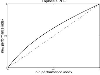
w.r.t. sources. This proves that, as it is well known, it is not possible to restore two gaussian sources. C.1.c Sources with Laplace’s distribution. We consider here that X1 and X2 are random signals with
PDF: p(x) = e−2|x| (its domain of definition is infinite unlike uniform PDF). Expressions of µ c1,j are: µc1,1=14(γ+1)2γ+12 µc1,2=14γ(γ+2)(γ+1)2
New ratio is ¯ ¯ ¯m11 m12 ¯ ¯ ¯ = ¯ ¯ ¯µc1,1 µc1,2 ¯ ¯ ¯ = ¯ ¯ ¯γ(γ+2)2γ+1 ¯ ¯
¯. For 0 < γ < 1, m11 < m12, ind(M(2)) > ind(M(1)). The new
performance index vs. the old one is shown on figure 2. There is only one attracting fixed-point (1,1) and a repelling fixed-point (0,0). 0 0.5 1 0 0.5 1 Laplace’s PDF
old performance index
new performance index
Fig. 2. Laplace’s PDF: new performance index vs. old performance index
Unlike the case of uniform PDF, performance index tends to 1 in lieu of 0. When convergence is finished, restored sources are linked to real sources through a rotation of angle 45◦. A corrective rotation of 45◦
must be applied at the end of convergence to balance this predictable behavior.
This behavior is particularly interesting since the algorithm does not converge to a separation state, but to an a priori known mixture state. It will be experimentally confirmed with more than two sources with Laplace’s PDF (cf. section VII).
C.1.d Conclusion. This section shows clearly how closely the behavior of our algorithm depends on PDF’s of sources. Three different behaviors have been observed:
• convergence to a separation state,
• convergence to an a priori known mixture state, • no convergence.
Now, let’s study convergence for any value of N .
C.2 Study for any number of sources
This section is devoted to a local study of convergence of the algorithm around points of interest, say fixed-points.
Starting from one line of M(1): M(1)
i =
h
αi1 ... αiN
i
, leads to the line of M(2): M(2)
i =
h
mi1 ... miN
i
. For the sake of simplicity, we will note Mi(1) = h α1 ... αN i , and Mi(2) = h m1 ... mN i
. As said before, it is always possible to normalize each equation of hyperplane: we will suppose that |α1| > |αi| ∀i: Mi(1) becomes
h
1 α2 ... αN
i .
From (14), ∀ j = 1, ..., N mj = 2 σ2 +∞ Z −∞ ... +∞ Z −∞ +∞ Z −PN i=2 αixi xjp(x1)dx1 p(x2)...p(xN)dx2...dxN. (15) As we want to study the behavior of the algorithm close to fixed-points, let’s see what happens if the initial line is h 1 α0 2 ... α0N i instead of h 1 α2 ... αN i
: then the final line is h m0 1 ... m0N i instead ofh m1 ... mN i . Then (see appendix A)
m0 j ∼ mj+σ22 +∞R −∞ ...+∞R −∞ (∆fx(α)p(fx(α))) xjp(x2)...p(xN)dx2...dxN, ∀j 6= 1 m0 1∼ m1+σ22 +∞R −∞ ...+∞R −∞ (∆fx(α)fx(α)p(fx(α))) p(x2)...p(xN)dx2...dxN. (16) with fx(α) = − N P i=2 αixi and ∆fx(α) = fx(α) − fx(α0).
Let us study this expression in the both following cases:
. around a separation point, . around other fixed-points.
C.2.a Study close to a point of separation. In this case h 1 α2 ... αN
i = h 1 0 ... 0 i and h 1 α0 2 ... α0N i =h 1 ε2 ... εN i
with |εi| ¿ 1: the observation yi = x1+
N
P
k=2
εkxk is almost
one of sources (here x1) with residual contribution of others. It comes (see appendix B) that the initial
ratio εj becomes m0 j m0 1 ∼2p(0) m1 εj.
Evolution to separation point depends on the term 2p(0)m
1 according to wether it is greater, equal or smaller
than 1; these quantity only depends on PDF’s of sources.
A direct application of this study around other fixed-points is given in appendix C: three particular cases (uniform, gaussian and Laplace’s PDF’s) are studied.
C.2.b Study of the algorithm around other fixed-points. Let us consider one observation Y1, i.e. one line
of the mixture matrix M , which is a linear mixture of q sources with the same coefficient: Y1=
q P k=1 Xk. h 1 ... 1 1 0 ... 0 i
(with q 1 and (N − q) 0) is a fixed-point of the algorithm. Then we wonder what will happen if we start from
h 1 ... 1 1 − ε 0 ... 0 i . Starting from h 1 ... 1 0 ... 0 i leads to h m1 ... mq−1 mq 0 ... 0 i
with obviously m1 = ... = mq−1 = mq. Starting from
h
1 ... 1 1 − ε 0 ... 0 i
, one step of the algorithm leads to h m0 1 ... m0q−1 m0q 0 ... 0 i with m0 1= ... = m0q−1.
According to paragraph VI-B.2, the presence of (N − q) 0 do not change future calculation of the following proof. There are always (N − q) 0 (at same position) in resulting mixture line. Study is the same than those of a q-length line
h 1 ... 1 1 − ε i . Noting m0 =m0q m0
1, three cases are possible:
• m0< 1 − ε: then algorithm tends to go away from the fixed-point; this is a repulsive fixed-point. • m0> 1 − ε: then algorithm tends to come closer to the fixed-point; this is an attractive fixed-point. • m0= 1 − ε: this is a neutral fixed-point.
In this case fx(α) = − q
P
i=2
xi and ∆fx(α) = εxq, and from equation (16),
m0 1∼ m1−σ22ε +∞R −∞ ... +∞R −∞ xq q P k=2 xk× p µ − q P k=2 xk ¶ p(x2)...p(xq)dx2...dxq, m0 j∼ m1+σ22ε +∞R −∞ ...+∞R −∞ xqxj× p µ −Pq k=2 xk ¶ p(x2)...p(xq)dx2...dxq, ∀j ∈ {2, ..., q}. (17) Noting ∆mi = m 0 i−m1 ε , we observe that ∆m1 = − q P k=2 ∆mk and q P k=1 m0 k = qm1. Furthermore, for
obvious reasons of symmetry, necessarily ∆m1= ... = ∆mq−1, implying ∆mq = −(q − 1)∆m1.
Let us find the conditions to be verified for m0 to be less than 1 − ε:
m0= m0q m0 1 < 1 − ε ⇐⇒ m1+ ε∆mq m1+ ε∆m1 < 1 − ε ⇐⇒ ∆mq− ∆m1 m1 < −1 ⇐⇒ ∆m1 m1 >1 q.
Evolution to separation point depends on wether the term ∆m1
m1 is greater, equal or smaller than
1
q; these
quantity depends on PDF’s of sources. We note that this quantity also depends on q. A study of evolution of this ratio according to q shows (see appendix D) that, according to PDF’s of sources, if a fixed-point is repulsive (resp. attractive) for a value of q, it remains repulsive (resp. attractive) for all value larger than q.
A direct application of this study around other fixed-points is given in appendix E: two particular cases (uniform and Laplace’s PDF’s) are studied.
Conclusion
Fixed-points of the algorithm can be divided in two classes, attractive and repulsive ones. For uniform PDF, the attractive fixed-point is [1 0 ... 1], i.e. separation state. For Laplace’s PDF, this is [1 ... 1]. The use of a perturbation method which consists in applying a known transformation (a rotation by example) to observations ensures that even if initial point is one of the repulsive fixed-points, convergence will lead to the attractive fixed-point. This method must be applied if after one step of algorithm, nothing has changed.
C.2.c Conclusion. This section of analysis of convergence of the algorithm stresses several important points:
• processing is done by line (nevertheless coherence of columns is ensured by orthogonalizing P at each
step because M is invertible by assumption).
• its behavior closely depends on PDF’s of sources: this limits naturally the range of proofs. Then study
has been done close to fixed-points: separation points and others.
• for uniform PDF, separation state is the sole attractive fixed-point: other fixed-points are repulsive. • for Laplace’s PDF, the sole attractive fixed-point is [1 ... 1].
• a perturbation method can be used to avoid freezing on a repulsive fixed-point.
In next section, computer simulation with digital signals will illustrate the power of this method. VII. Simulations
Algorithm has been tested with digital signals. Throughout this section all signals will be understood to have the same PSD (i.i.d.), unless the contrary is specifically stated. Theoretically, sources and mixture matrix are unknown; however, as performed usually, we will use this information to quantify the relevance of results.
Sources and observations can be represented by N -by-L matrices:
X =³X1 X2 ... XN
´T
and Y =³Y1 Y2 ... YN
´T
where Xi is an L-dimensional vector
³
xi(1) xi(2) ... xi(L)
´T
.
A. Practical considerations
Simulations are completed with matlabr. Matlab functions like rand and randn are used respectively
to create time samples of uniformly distributed (as well as binary or four states) or gaussian sources. In appendix F are given the processes to generate sources with a Laplace’s PDF and to generate sources with same PDF but different PSD.
Practically, to reach the condition Yi> 0 (i.e.
PN
k=1αikXk > 0), we process an extraction of a sequence
from observation Yi; for example let’s use the first one Y1: we select indices k=1,...L for which y1(k) is
positive, and create an Lc1-dimensional vector c1 whose entries are these indices. Then, for j = 1, ...N ,
we are able to create the jthextracted observations Y
c1,j (which is an Lc1-length vector) defined by
Yc1,j =
³
yj(c1(1)) ... yj(c1(Lc1))
´T
,
and conditional observations Yc1 (which is a N × Lc1 matrix): Yc1 =
³ Yc1,1 · · · Yc1,N ´T . example : Y = 1 4 −1 3 −1 −5 −4 5 1 −5 3 2 ; then c1= ³ 1 2 4 ´ and Yc1 = 1 4 3 −4 5 −5 .
B. Results and comments
For a chosen value of N and given types of PDF (specified in each case), iterations are stopped when the value of ind(P ) is less than a small value ε chosen beforehand. To quantify results, we choose the
following criterions: the value of ind(M(∞)) where M(∞) is the mixture matrix at the end of convergence,
and the mean square error (mse) between real and restored sources. Values presented in the table below are average values obtained from 500 experiences. The mean number of iterations necessary to reach the stopping condition is also given.
For each realization, mixture matrix (invertible) and sources are chosen at random.
. Sources with a uniform PDF
Results are summarized in Table I.
TABLE I
Sources with a uniform PDF
N ind(M(∞)) Number of
iterations
ind(P ) mse (on one source) 2 4.1 10−5 18 ± 6 2.3 10−6 1.6 10−5± 9.0 10−6
2† 3.5 10−5 20 ± 7 3.9 10−6 1.3 10−5± 7.8 10−6
4 1.1 10−4 30 ± 9 9.8 10−6 1.9 10−4± 3.7 10−5
10 1.9 10−4 52 ± 15 1.9 10−5 1.3 10−3± 8.6 10−5
† This case illustrates that the algorithm works as well with sources which have different PSD’s.
remark concerning the robustness w.r.t. number of sources
Results obtained for N = 10 are convincing; the algorithm is robust w.r.t. the number of sources, contrary to H.O.S. methods which fail quickly when N increases. Examples with 40 uniformly distributed sources have also been processed successfully.
Let’s note that simulations with sources with a limited number of states (digital communications) have been realized. Results are very good and convergence is all the better when the number of states decreases. In such cases, the mean square error need not to be very small, and a reasonable small value can easily be neglected a posteriori.
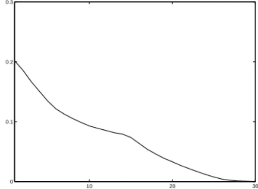
remark The mean number of iterations necessary to reach the stopping condition is given with a standard deviation. Nevertheless, this information is incomplete as it does not permit to realize how performance index converges. Hereafter are given two examples of this evolution versus the iteration number in cases of 2 and 10 uniformly distributed sources (figures 3 and 4).
10 20 0
0.5 1
Fig. 3. N=2 : example of evolution of performance index vs. number of iterations
10 20 30
0 0.1 0.2 0.3
Fig. 4. N=10 : example of evolution of performance index vs. number of iterations
. Sources with a Laplace’s PDF
Results presented take into consideration the final correction described in section VI-C.1.c. In the case
N = 3, convergence leads to the mixture state [1 1 1]. Real sources are retrieved by 2 successive rotations
(of angle arctan√2 and 45◦) about appropriate orthogonal axis. Results are summarized in Table II.
TABLE II
Sources with a Laplace’s PDF
N ind(M(∞)) Number of
iterations
ind(P ) mse (on one source) 2 8.8 10−5 23 ± 8 1.9 10−5 7.4 10−7± 5.3 10−7
3 1.2 10−3 50 ± 16 1.0 10−5 1.0 10−5± 1.9 10−5
. Sources with different PDF’s
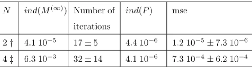
Result presented here aims at illustrating that the method proposed can as well process mixtures of sources with different PDF’s (provided that at the most one gaussian source is present). Results are summarized in Table III.
TABLE III
Sources with different PDF
N ind(M(∞)) Number of
iterations
ind(P ) mse
2 † 4.1 10−5 17 ± 5 4.4 10−6 1.2 10−5± 7.3 10−6
4 ‡ 6.3 10−3 32 ± 14 4.1 10−6 7.3 10−4± 6.2 10−4 † first source has a uniform PDF, second one a Laplace’s PDF.
‡ sources have respectively a uniform PDF, a uniform PDF with a different PSD, a Laplace’s PDF and
a gaussian PDF.
C. Comparison with a classical HOS method
Let’s compare numerically our algorithm’s behavior to a classical HOS one, say JADE algorithm. This comparison consists in launching the both algorithms for identical data (sources and mixture matrix).
The criterion to evaluate these methods is the value of ϑ = ind¡M(∞)¢, performance index of the final
mixture matrix.
Tables above give results obtained with the both methods for several kinds of sources’ PDF’s. When an acceptable separation state is reached, CPU times are presented to give the reader a rough idea of time convergence: its significance does not lie in its absolute values but in a comparison between magnitudes for the both methods.
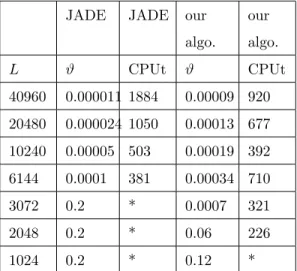
It sometimes happens that JADE algorithm converges to a bad solution (e.g. in Table IV for N = 40 and L = 3072 where ind¡M(∞)¢= 0.2) ; this case is indicated by an asterisk. Let’s note that a value of
ind¡M(∞)¢greater than 0.01 is a bad one (separation is far from being reached).
For a given number of sources N , let’s see what happens as the number of time samples L decreases.
. Uniformly distributed sources
TABLE IV
Comparison with HOS method for 40 uniformly distributed sources
JADE JADE our algo. our algo. L ϑ CPUt ϑ CPUt 40960 0.000011 1884 0.00009 920 20480 0.000024 1050 0.00013 677 10240 0.00005 503 0.00019 392 6144 0.0001 381 0.00034 710 3072 0.2 * 0.0007 321 2048 0.2 * 0.06 226 1024 0.2 * 0.12 *
We can observe in this table that, as expected, for a given value of N , the quality of results decreases with L. When L is too small, both methods fail.
. Binary sources
Let us consider 40 binary sources, i.e. each time sample is equal to -1 or +1. Results are summarized in Table V.
TABLE V
Comparison with HOS method for 40 binary sources
JADE JADE our algo. our algo. L ϑ CPUt ϑ CPUt 4096 0.00007 335 0.00013 605 2048 0.00013 402 0.00026 229 1536 0.205 * 0.00034 175 1024 0.225 * 0.00050 131 512 * * 0.1 72
. Four states sources
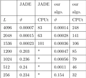
Let us consider 30 sources which can take 4 values (-1, -0.5, 0.5 and 1) with an identical probability. Results are summarized in Table VI.
TABLE VI
Comparison with HOS method for 30 Four states sources
JADE JADE our algo. our algo. L ϑ CPUt ϑ CPUt 4096 0.00007 83 0.00014 248 2048 0.00015 63 0.00028 141 1536 0.00023 101 0.00036 106 1200 0.203 * 0.00047 85 1024 0.236 * 0.00056 79 512 0.24 * 0.0011 46 256 0.234 * 0.154 32 Conclusion
Some conclusions can be deduced from the observation of these few numerical experimental results. For a given number of sources N , both methods work all the better that the number of time samples
L of each source increases: the price to pay is increasing CPU time. In fact, when N increases, L must
increase significantly for results to stay as satisfactory.
For a large value of L (relatively to N ), JADE algorithm gives better results: in such a case, JADE algorithm is very efficient and it is difficult to compete with it.
But, as said before, the advantage of our method appears when N increases while L does not (or equivalently when L decreases while N is fixed). A decreasing value of L involves a slow degradation of results; under a threshold of L, different according to the algorithm, the algorithm fails. The threshold for JADE algorithm is higher than for ours, thus there exists an area of values of L for which JADE algorithm totally fails while ours continues to give acceptable results. In this area, our algorithm brings a substantial improvement.
Naturally when L is too small, both methods fail.
VIII. Conclusions
In this paper we present a new method for blind source separation problem when PSD’s of sources are the same; in such cases it is well known that second-order methods are ineffective. In fact, the method proposed does not depend on PSD’s of sources and also gives good results in the case of different PSD’s. Thus this algorithm can be used for both cases.
The method proposed presents several advantages:
• Contrary to geometrical methods [2] [25][26] or neural network methods [3][15], it can process sources
• Calculations are limited to only first and second-order moments.
• It is robust w.r.t. the number of sources (relatively to the number of time samples of each source). • Despite a presentation which could seem complicated, the algorithm is very easy to program and
neces-sitates few calculation.
For reasons explained in the paper we have limited our study to symmetrical PDF’s. Two classes of signals have been more precisely detailed: uniformly distributed sources (digital communications) and sources with a Laplace’s PDF.
The state reached at the end of convergence depends only on PDF’s of sources: this state can be a separation state (e.g. uniformly distributed sources) or an a priori known mixture state (e.g. sources with a Laplace’s PDF).
Speed of convergence is different according to PDF (in fact it depends on the distance to a gaussian PDF) and number of sources; for example, for sources with a triangular PDF, convergence is slower than with uniform ones.
Practically convergence is always reached. However when the number of sources grows, mean-square error is larger; as our objective is not to find exactly sources, but an approximation as satisfying as possible, this is quite acceptable for numerous engineering applications.
For uniformly distributed sources (with any number of states) results are very convincing: the algorithm converges directly to a separation state. In this case, it will be doubtless possible to establish a link with contrast functions [24].
Numerical comparisons with a commonly used HOS method (JADE) are provided. They show that for a given number of sources, our method continues to give acceptable results while JADE algorithm when the number of time samples available decreases.
On the other hand, for sources with Laplace’s PDF, as at the end of convergence we obtain an a priori known mixture state, a final operation is necessary to reach the separation state: in this case it is hardly possible to talk of contrast function. However a generalization of contrast functions could be glimpsed in the light of this particular example. As a prospect, this question needs to be examined in more details: much work remains to be done concerning a link between our method and contrast functions.
Another prospect is the study of convergence of the algorithm when PDF’s of sources are no more sym-metric. Also a theoretical study of links with HOS methods must be performed in the future. Obviously, application of this algorithm (with adaptations) to convolutive mixture problem with sensor noise must be the subject of a detailed study in the near future.