HAL Id: hal-01077801
https://hal.archives-ouvertes.fr/hal-01077801
Submitted on 27 Oct 2014
HAL is a multi-disciplinary open access
archive for the deposit and dissemination of
sci-entific research documents, whether they are
pub-lished or not. The documents may come from
teaching and research institutions in France or
abroad, or from public or private research centers.
L’archive ouverte pluridisciplinaire HAL, est
destinée au dépôt et à la diffusion de documents
scientifiques de niveau recherche, publiés ou non,
émanant des établissements d’enseignement et de
recherche français ou étrangers, des laboratoires
publics ou privés.
Data Mining by NonNegative Tensor Approximation
Rodrigo Cabral Farias, Pierre Comon, Roland Redon
To cite this version:
Rodrigo Cabral Farias, Pierre Comon, Roland Redon. Data Mining by NonNegative Tensor
Approxi-mation. MLSP 2014 - IEEE 24th International Workshop on Machine Learning for Signal Processing,
Sep 2014, Reims, France. �hal-01077801�
2014 IEEE INTERNATIONAL WORKSHOP ON MACHINE LEARNING FOR SIGNAL PROCESSING, SEPT. 21–24, 2014, REIMS, FRANCE
DATA MINING BY NONNEGATIVE TENSOR APPROXIMATION
Rodrigo Cabral Farias, Pierre Comon
∗GIPSA-lab, CNRS UMR5216,
11, rue des Math´ematiques, BP 46
38402 Saint Martin d’H`eres, France
{rodrigo.cabral-farias, pierre.comon}@gipsa-lab.grenoble-inp.fr
Roland Redon
Lab. PROTEE, EA3819
Universit´e de Toulon,
83957 La Garde, France
ABSTRACT
Inferring multilinear dependences within multi-way data can be performed by tensor decompositions. Because of the pres-ence of noise or modeling errors, the problem actually re-quires an approximation of lower rank. We concentrate on the case of real 3-way data arrays with nonnegative values, and propose an unconstrained algorithm resorting to an hy-perspherical parameterization implemented in a novel way, and to a global line search. To illustrate the contribution, we report computer experiments allowing to detect and identify toxic molecules in a solvent with the help of fluorescent spec-troscopy measurements.
Index Terms— muti-way ; tensor ; CP ; low-rank ; ap-proximation ; nonnegative ; line search ; fluorescence ; HAP
1. INTRODUCTION
Tensor decompositions are emerging as an alternative tool for machine learning and data mining. They permit to (but are also limited to) find multilinear dependences between hidden variables. For instance, they have been already used in the field of blind source separation, but less used as a determinis-tic tool for mining data.
In the present framework, we shall concentrate on real nonnegative data, which are organized in the form of a multi-way array. Several applications have already been identified, which fit in this framework, including machine learning [1], internet connection analysis [2, 3], hyperspectral imaging [4], spectrography [5], as well as a few others [6, 7]. Our de-scription will focus on 3-way fluorescence spectrography, but could of course apply to arrays of higher order and to other application fields where nonnegativity is important.
Notation Vectors will be distinguished from scalar num-bers by bold lowercases, e.g. v; matrix and tensor arrays will be denoted by bold and calligraphic uppercases, respectively,
e.g. Aand T . Array entries are real scalar numbers, and are
denoted by plain letters, e.g. vi,Ajk,T`mn, for the previ-ous vector, matrix or tensor examples. Vectors will be
repre-⇤This work has been funded by the European Research Council under the
7th Framework Programme FP7/2007–2013 Grant Agreement no. 320594.
sented by column arrays of coordinates. A ! B will denote the element-wise (Hadamard) product between two matrices of same dimensions,⌦ will denote the outer product between arrays, e.g. v⌦ A ⌦ T is the object whose coordinates are viAjkT`mn. These are the notations assumed in e.g. [8].
2. TENSOR APPROXIMATION 2.1. Tensor decomposition
The objective is to decompose a3-way data array Y in a fi-nite sum of outer products of vectors (also known as tensor products). For example, if we consider an array of real val-ues of size I ⇥ J ⇥ K, then we want to find the vectors ar = [A1r, · · · AIr]> 2 RI, br = [B1r, · · · BJ r]> 2 RJ and cr = [C1r, · · · CKr]> 2 RK withr 2 {1, · · · , R} for which Yijk= R X r=1 AirBjrCkr, (1)
or equivalently using the outer product
Y = R X r=1
ar⌦ br⌦ cr. (2)
IfR is the smallest number of components necessary to ex-actly decompose Y, then (2) is called the canonical polyadic (CP) decomposition ofY; see [5, 6, 8] and references therein. Most of the time, Y cannot be exactly decomposed as in (2) for the desiredR, either because the actual model behind Y is not multilinear (linear in ar, brand crindividually), or because the data are noisy. In this case, for a givenR, the goal is to find{ar, br, cr, 1 r R} that best approxi-mate the original array, for example, by solving the following minimization problem minimize Υ = " " " " Y− PR r=1 ar⌦ br⌦ cr " " " " 2 2 w.r.t. A= [a1, · · · aR] 2 RI⇥R,
B= [b1, · · · bR] 2 RJ ⇥R, C= [c1, · · · cR] 2 RK⇥R,
(P.1)
c
wherek · k2is the Frobenius norm: kT k2 =qP
i,j,kTijk2 . Matrices A, B, and C are commonly called loading matrices [5].
Several approaches may be found in the literature, which search for a solution of problem (P.1). They range from simple alternating algorithms like the well-known alternating least squares (ALS) [5] to all-at-once minimization proce-dures like gradient descent, conjugate gradient and quasi-Newton algorithms [9, 10, 4, 11]. Interestingly, a solution for problem (P.1) does not necessarily exist [12], and, as a consequence, searching for it is an ill-posed problem.
2.2. Nonnegative CP and quadratic parameterization A particular case for which problem (P.1) is well-posed is when the vectors in A, B and C are nonnegative. In this case, it can be shown that a solution exists [13]. Not only this instance of the problem is well-posed, but it also naturally ap-pears in many applications such as fluorescence spectrometry, as pointed out in Section 1. For these reasons, in what follows, we focus on the nonnegative version of problem (P.1), which may be stated as follows, for a given nonnegative tensor Y:
minimize Υ = " " " " Y−PR r=1 ar⌦ br⌦ cr " " " " 2 2 w.r.t. A, B and C, subject to A⌫ 0, B ⌫ 0 and C ⌫ 0, (P.2)
where F⌫ 0 means that all elements of F are nonnegative. Common methods solving (P.2) include ALS with active sets [14, p. 170], minimization methods with logarithmic penalty functions [9] and extensions of algorithms used for nonnegative matrix factorization [15], [16] such as ALS, reg-ularized ALS with projection, projected gradient, accelerated proximal gradient, gradient with nonnegative multiplicative update and projected quasi-Newton techniques.
Instead of solving the minimization problem (P.2), an in-teresting approach studied in [11] consists in reparameter-izing the problem with the loading matrices A0 2 RI⇥R, B02 RJ ⇥Rand C0 2 RK⇥Rsuch that
A= A0! A0 = 2 6 4 a2 1,1 · · · a21,R .. . ... a2 I,1 a2I,R 3 7 5, B= B0! B0 and C= C0! C0. (3)
Note that with this reparameterization the original minimiza-tion problem becomes unconstrained:
minimize " " " " Y− R P r=1 (a0 r! a0r) ⌦ (b0r! b0r) ⌦ (c0r! c0r) " " " " 2 2 w.r.t. A0, B0and C0, (P.3) since the components of the approximation are now non-negative by construction. As a consequence, this approach
does not require the introduction of projection techniques; for example, in [11] a conjugate gradient technique for uncon-strained problems is used to solve problem (P.3).
2.3. Unit norm constraint and spherical parameteriza-tion
The nonnegativity constraint imposed above allows to guaran-tee the existence of a solution, but an issue that still persists is the lack of uniqueness of the parameterization. Non unique-ness of the solution comes from multiple ambiguities inherent in the multilinear model (P.1), which persist in (P.3).
The first ambiguity put forward in the literature is that of permutation, since the order in which the R terms are summed has no influence on the result. Actually, this issue is irrelevant in parameter estimation, even if it is important when assessing performance in computer experiments. On the other hand, there remains a scaling ambiguity, induced by the multiplicative aspect within components. In fact, the tensor a⌦ b ⌦ c can be equally represented by the triplets of vectors(a, b, c) or (λ1a, λ2b, c/λ1λ2), for any nonzero numbers{λ1, λ2}; this indeterminacy is inherent in the defi-nition of tensor spaces [8]. Contrary to permutation, scaling can have an effect on optimization algorithms used to solve (P.2). In particular, it can make iterations continuously move between various scaling-equivalent solutions. In practice, it is useful to fix these ambiguities.
To solve this issue, we can impose that all the columns of A and B have a unitL1norm, as these matrices are already restricted to have nonnegative elements:
kark1= 1 and kbrk1= 1, forr = {1, · · · , R} . (4) On the other hand, matrix C is left unconstrained.
These L1-norm constraints impose the following L2-norm constraints in the nonnegative reparameterization (P.3):
ka0 rk 2 2= 1 and kb0rk 2 2= 1, forr = {1, · · · , R} . (5) As a consequence, each column vector of A0 and B0 is con-strained to lie on the unitL2-hypersphere. This can also be imposed by a parameterization, which consists of describing them using polar coordinates, namely by angles. For exam-ple, any vector a0 withI components can be parameterized with angles θ= [✓1 · · · , ✓I−1]>as
"
cos ✓1, cos ✓2sin ✓1, . . . , cos ✓I−1 I−2 Y i=1 sin ✓i, I−1 Y i=1 sin ✓i #>
But since these angles can be restricted to belong to the in-terval[0, ⇡/2], one can instead use their tangent ti2 [0, 1[, since there exists a bijection relating them: cos2✓i = (1 + t2
i)−1andsin
2✓i = t2
i(1 + t2i)−1. Finally, a generic vector a = a0! a0with nonnegative entries and unitL1-norm can
be written as " 1 1 + t2 1 , 1 1 + t2 2 t2 1 1 + t2 1 , . . . 1 1 + t2 I−1 I−2 Y i=1 t2 i 1 + t2 i , I−1 Y i=1 t2 i 1 + t2 i #> ,
But it turns out that there is an even simpler and obvious way to do this, which will present significant advantages. In fact consider the simpler parameterization
1
1 +PIi=2⌧2 ⇥1, ⌧ 2
2, ⌧32, . . . , ⌧I2⇤ , ⌧i2 [0, 1[. This parameterization also allows to represent any nonnega-tive vector on the unitL1-hypersphere. There is a relationship between{ti} and {⌧i}, but it is irrelevant in our discussion. Clearly, there areI possible such parameterizations of the I-dimensional hypersphere, depending on the place where the value 1 is imposed. We assumed the value 1 was set in the first entry, but the reasoning is the same with a different location.
The inconvenience of this solution, which is also shared by tangentsti, is that all⌧i’s need to tend to infinity in order to approach zero in the first coordinate. The consequence is that zero cannot be exactly obtained, and that this parameteri-zation is valid only generically. For this reason, we shall now consider projective coordinates:
1 PI
i=1⌧i2 ⇥⌧2
1, ⌧22, . . . , ⌧I2⇤ . (6) Clearly, we have now too many parameters, and the pa-rameter vector(⌧1, . . . ⌧I) corresponds to the same point as λ(⌧1, . . . ⌧I) for any nonzero nonnegative λ. This is precisely what allows not only to reach all possible values, but also to better condition the parameterization because we may now impose|⌧i| 2 [0, 1]. In practice, setting λ = |⌧max|−1, the inverse of the largest|⌧i|, will yield the best conditioning. In the remainder, we refer to this parameterization technique as Parameterization of Positive Orthant Hyperspheres (PAPOH). Then problem (P.3) reduces to:
minimize Υdef= " " " " Y−PR r=1 Dr " " " " 2 2 , w.r.t. α, β and γ, (P.4)
where Drdenote decomposable (rank-1) tensors Drdef= ar(αr) ⌦ br(βr) ⌦ cr(γr),
where ar(αr) and br(βr) are parameterized as in (6); vector (↵1r, . . . ↵Ir)>is denoted by αr, ar(αr) = P1 i↵2ir ⇥↵2 1r, . . . ↵2Ir ⇤> , max i ↵ 2 ir= 1, (7) α is the set ofR vectors αr, and a similar notation is used for βr, β, γrand γ. Here the entries of cr(γr) are simply Ckr = γ2
kr, where for notation homogeneityγkr is an Ersatz ofC0
kr.
2.4. Fundamental difference with projection
The algorithm proposed in this contribution will choose at
ev-ery iterationthe most appropriate parameterization by setting
to1 the absolute value of one parameter in every vector αr and βr, 1 r R, as depicted in (7). Every unit-norm vector with nonnegative entries may hence have a 1 in the numerator at a different location, and this may vary with iter-ations.
There is a fundamental difference between this parame-terization (PAPOH) and projection. In fact, the iterations we produce are by construction all on the hypersphere, and the most well conditioned parameterization is chosen at very it-eration. On the other hand in projected iterative algorithms, iterations are generated outside the hypersphere and are pro-jected onto it at every iteration.
3. ALGORITHM 3.1. Parameter update
To solve (P.4), we use a conjugate gradient algorithm. Let
xt def = 2 4 ˆ α ˆ β ˆ γ 3 5 t and gtdef= 2 4 rΥα rΥβ rΥγ 3 5 t .
For this algorithm the estimatesα, ˆˆ β and γ are updated atˆ iterationt using the Pollak-Ribi`ere update formula:
xt+1 = xt− µtdt,
⌫t = (gt+1− gt)>gt+1/||gt||22, dt+1 = Mtgt+1− ⌫tdt,
whereµtis a variable step size, dtis the descent direction, which is initialized to d1= g1, and Mtis a preconditioning matrix, usually diagonal, which we have set to identity in the present paper.
3.2. Gradient expressions
At each iterationt, one index i(r, t) (resp. j(r, t)) in every vector αr(resp. βr) is chosen, so that↵2
i(r,t),r = 1 (resp. β2
j(r,t),r = 1). The gradient w.r.t. ↵i(r,t),r does not exist at iterationt, and in practice it may be set to zero since ↵2
i(r,t),r remains equal to 1. We eventually have the following deriva-tives: fori 6= i(r, t) @Air @↵ir = 2 ↵iruir (P q↵2qr)2 , (8) fori 62 {i(r, t), p} @Apr @↵ir = −2 ↵ir↵2 pr (P q↵2qr)2 , (9)
with uirdef=P q6=i↵2qr, and forp = i(r, t) @Apr
@↵ir = −2 ↵ir (P
q↵2qr)2
Following the notation assumed for αr in (7), βjr andγkr will denote thejth and kth entries of vectors βrand γr, re-spectively. Now defineEijk= Yijk−P
rAirBjrCkr, so that Υ = ||E||2. Then,8p, i, 1 p I, i 2 {1, . . . I} − {i(r, t)}:
@Υ @↵ir = −2 X pjk Epjk@Apr @↵irBjrCkr. (11)
Similar expressions hold for β, by exchanging the roles of A and B, with br = βr! βr/||βr||22 as in (7). For the third loading matrix, there is no normalization, and cr = γr! γr so that @Υ @γkr = −4 X ij EijkAirBjrγkr. (12)
3.3. Exact Line Search (ELS) by polynomial fitting Since the objective functionΥ defined in (P.4) is a rational function in the unknown parameters, for any fixed direction g= [g↵, gβ, gγ]>, defined e.g. by the gradient, the station-ary points ofΥ with respect to µtare the roots of a polynomial ⇡(µ) in µt. This is a great advantage of the parameterization we have assumed: the value of the step sizeµtyielding the
globallyminimal value of the objective along the search
di-rection can be found. More precisely, we proceed in three steps:
1. Computation of the coefficients of the rational
func-tion. From (1) and (6), it can be seen that the objective
takes the form
Υ(α + µg↵, β + µgβ, γ + µgγ) = X ijk " Yijk− R X r=1 `2 A,ir(µ) qA,r(µ) `2 B,jr(µ) qB,r(µ) ` 2 C,kr(µ) #2 ,
where`A,ir,`B,jrand`C,krare linear forms, andqA,r andqB,rare quadratic forms inµ.
2. Finding the roots of the first derivative: @Υ
@µ = 0 , ⇡(µ) = 0, (13) where the exact expression of⇡ can be obtained from those of the above linear and quadratic forms.
3. Finding the root corresponding to the global minimum: just select the best root by evaluatingΥ at those values. However, to spare some computational load, this optimal step size does not need to be computed at every iteration, but can be executed only cyclically, for instance at everyIJKR iterations, or just before termination, with the hope that it could help escape from local minima in case the algorithm is stuck.
3.4. Complexity
Following the usual practice, the computational complexity is assimilated to the number of multiplications, being under-stood that a floating point operation (flop) is implemented as a multiplication followed by an addition, and that the number of multiplications is generally of same order as the number of additions [17].
Update rule. The update of A, B and C is dominated by the gradient computation, whereas the complexity involved by (8-9) is negligible. In fact, the computation of the gradi-ent requires the contraction of tensorEijk over two or three indices as shown in (11) and (12). More precisely, the update (8) requires an order ofO(IJKR(I + J + 1)) multiplies.
Line Search. Next, the computation of the globally op-timal step size (ELS) is dominated by the calculation of the coefficients of polynomial⇡(µ); the computation of its roots is comparatively negligible. More precisely, dropping indices for an easier writing, polynomial⇡ takes the expression:
⇡(µ) = R X r=1 2 4 Y n6=r q2Anq2Bn 3 5(2Fr− Gr) with Fr = qArqBr X ijk Eijk[`A`0A`B2`2C+ `2A`B`0B`2C+ `2A`2B`C`0C] Gr = (qAr0 qBr+ qArq0Br) X ijk Eijk`2A`2B`2C.
If we assume that the Fourier transform is not used to compute the product of two polynomials of degreem and n, with say 0 < m n, then the complexity of the product is (n − m)(m + 1) + (m + 1)(m + 2)/2 flops. On this basis, one can then show that computing all the coefficients of⇡(µ) requires a computational complexity which increases asO(IJKR).
3.5. Initialization and stopping
The initial value is drawn randomly and belongs to the feasi-ble set; that is, every parameter vector aror bris nonnegative belongs to the unitL1hypersphere.
One defines a maximal number of iterations,tmax, and a minimal relative variation of the objective,". The iterations are stopped if one of the two conditions below are satisfied:
1. Maximal number of iterations reached:t ≥ tmax 2. The relative variations of the objective function have
become negligible:|Υt+1− Υt|Υ−1t+1< ".
4. COMPUTER EXPERIMENTS
In what follows we test five different algorithms used to find tensor approximations: alternating least squares (ALS) with-out nonnegativity constraints1, alternating least squares with
1A projection is carried out only at the last iteration after normalizing the
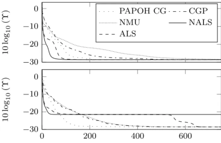
projection on the nonnegative orthant (NALS), gradient with nonnegative multiplicative update (NMU), conjugate gradient using the parameterization with squares (CGP), and conju-gate gradient with PAPOH (PAPOH CG). The true nonnega-tive CP model has random elements such thatA and B have unitL1norm. The model dimensions areI = 20, J = 20, K = 15 and R = 8 and it is measured with independent identically distributed (i.i.d.) Gaussian noise with standard deviation σ= 5 ⇥ 10−4. Algorithm initialization is also ran-dom but equal for all algorithms. In the simulations, we used the NMU algorithm from the MATLAB Tensor Toolbox [18]. Simulation results for two different realizations are shown in Fig.1, where the reconstruction error is plotted (in dB) as a function of the number of iterations. Note that if we com-pare the performance of the gradient-based algorithms, NMU is the slowest and PAPOH CG is the fastest. Notice that the alternating algorithms can be either fast or slow depending on the initial conditions. In the second realization we can see that NALS is blocked in a point far from the optimum.
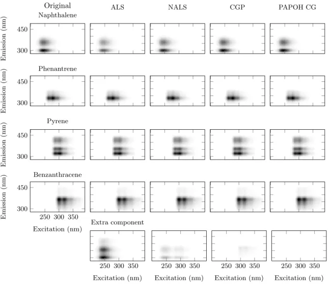
The data used for the second test are generated by arti-ficially mixing fluorescence excitation-emission spectra rep-resentative of 4 different polycyclic aromatic hydrocarbons (PAH): naphthalene, phenanthrene, pyrene, benzanthracene. The mixing matrices (10 in the present case) are generated randomly with nonnegative values. The algorithms are tested supposingR = 5 to simulate a misdetection of the number of solutes. The original and reconstructed spectra are shown in Fig.2 after5000 iterations, and plotted as a function of wave-lengths, as usual in the field of chemometrics. The results for the standard ALS algorithm are shown by normalizing and projecting the final result on the nonnegative orthant (but its iterations are unconstrained). Results for the NMU algorithm are not shown due to space limitation.
One can observe that the ALS algorithms generate a spu-rious component that does not exist. On the other hand, the CGP of [11] and PAPOH CG make a good job. If we look at the sums of the squared errors on the parameters (and not on the tensor reconstruction) we can clearly see the differences. They are the following: ALS -2.00 ⇥ 10−3, NALS -2.36 ⇥ 10−4, CGP -2.82 ⇥ 10−5 and PAPOH CG -3.12 ⇥ 10−9. In practice, the gradient-based algorithms can be made even more robust to a misdetection of the number of solutes by adding an approximation of the mixed pseudo normL1,0as a penalty term (this will be reported in another paper). This can hardly be done in the ALS approach.
5. CONCLUSIONS
TheL1norm has been chosen since it is the natural norm for vectors with nonnegative entries. This led to a simple param-eterization of the intersection of the unitL1-hypersphere and the nonnegative cone, which is symmetric and expressed as a rational function. Among useful by-products, we have sim-pler gradient expressions, a conditioning easy to monitor, and a step size that can be globally optimized. The efficiency of
−30 −20 −10 0 10 log 10 (Υ ) PAPOH CG CGP NMU NALS ALS 0 200 400 600 −30 −20 −10 0 10 log 10 (Υ )
Fig. 1. Cost functionΥ (dB) versus iterations. The true CP model is generated randomly such that all of its elements are nonnegative and the columns of the factors A and B have unitL1norm. The results obtained with two realizations are shown. The CP model is of dimension20 ⇥ 20 ⇥ 15, with rankR = 8. The model is measured with i.i.d. Gaussian noise with standard deviation σ= 5 ⇥ 10−4.
this algorithm is illustrated by a problem of fluorescence spec-troscopy, which is important in environmental sciences. The CP decomposition of the nonnegative data tensor into rank-one terms permits to identify pure solutes, such as toxic poly-cyclic aromatic hydrocarbons highly diluted in water. In par-ticular, the proposed algorithm better detects the number of fluorescent solutes, and hence better identifies them via their spectrum.
6. REFERENCES
[1] A. Shashua and T. Hazan, “Non-negative tensor factorization with applications to statistics and computer vision,” in 22nd
Int. Conf. Machine Learning, Bonn, 2005, pp. 792–799.
[2] D. M. Dunlavy, T. G. Kolda, and E. Acar, “Temporal link prediction using matrix and tensor factorizations,” ACM Trans.
Knowledge Discov. Data, vol. 5, no. 2, Feb. 2011.
[3] E. Acar and B.Yener, “Unsupervised multiway data analysis: A literature survey,” IEEE Transactions on Knowledge and
Data Engineering, vol. 21, no. 1, pp. 6–20, 2009.
[4] P. Zhang, H. Wang, R. Plemmons, and P. Pauca, “Tensor meth-ods for hyperspectral data analysis: A space object material identification study,” J. Optical Soc. Amer., vol. 25, no. 12, pp. 3001–3012, Dec. 2008.
[5] A. Smilde, R. Bro, and P. Geladi, Multi-Way Analysis, Wiley, Chichester UK, 2004.
[6] T. G. Kolda and B. W. Bader, “Tensor decompositions and applications,” SIAM Review, vol. 51, no. 3, pp. 455–500, 2009. [7] L-H. Lim and P. Comon, “Nonnegative approximations of nonnegative tensors,” Jour. Chemometrics, vol. 23, pp. 432– 441, Aug. 2009, hal-00410056.
[8] P. Comon, “Tensors: a brief introduction,” IEEE Sig. Proc.
Magazine, vol.31, no.3, May 2014, special issue on BSS.
300 450 E m is si o n (n m ) Naphthalene Original 300 450 E m is si o n (n m ) Phenantrene 300 450 E m is si o n (n m ) Pyrene 250 300 350 300 450 Excitation (nm) E m is si o n (n m ) Benzanthracene ALS 250 300 350 Excitation (nm) Extra component NALS 250 300 350 Excitation (nm) CGP 250 300 350 Excitation (nm) PAPOH CG 250 300 350 Excitation (nm)
Fig. 2. Fluorescence spectra obtained with four different algorithms: alternating least squares (ALS) without nonnegativity constraints (negative values appear as white), ALS with projection on the nonnegative orthant (NALS), nonnegative conjugate gradient (CGP), and conjugate gradient with Parameterization of Positive Orthant Hyperspheres (PAPOH CG). As it is indicated in the column “Original”, where the original unmixed spectra are shown, the spectra are representative of4 different polycyclic aromatic hydrocarbons (PAH): naphthalene, phenanthrene, pyrene, benzanthracene. The algorithms are tested supposingR = 5 to simulate a misdetection of the number of components, the5thline thus represents an additional artificial component that may have been estimated. The black color represents the largest intensity value and white is zero.
[9] P. Paatero, “A weighted non-negative least squares algorithm for three-way ’parafac’ factor analysis,” Chemo. Intel. Lab.
Syst., vol.38, no.2, pp. 223–242, 1997.
[10] P. Comon, X. Luciani, and A. L. F. De Almeida, “Tensor decompositions, alternating least squares and other tales,” J.
Chemometrics, vol.23, pp. 393–405, 2009, hal-00410057.
[11] J.-P. Royer, N. Thirion-Moreau, and P. Comon, “Comput-ing the polyadic decomposition of nonnegative third order ten-sors,” Signal Processing, vol. 91, no.9, pp. 2159–2171, 2011. [12] V. De Silva and L.-H. Lim, “Tensor rank and the ill-posedness
of the best low-rank approximation problem,” SIAM J. Matrix
Ana. Appl., vol.30, no.3, pp. 1084–1127, 2008.
[13] L.-H. Lim and P. Comon, “Nonnegative approximations of nonnegative tensors,” Journal of Chemometrics, vol.23, no.7-8, pp. 432–441, 2009.
[14] R. Bro, Multi-way analysis in the food industry: models,
al-gorithms, and applications, Ph.D. thesis, University of
Ams-terdam, The Netherlands, 1998.
[15] A. Cichocki, R. Zdunek, A. H. Phan, and S.-i. Amari,
Non-negative matrix and tensor factorizations: applications to ex-ploratory multi-way data analysis and blind source separa-tion, John Wiley & Sons, 2009.
[16] G. Zhou, A. Cichocki, Q. Zhao, and S. Xie, “Nonnegative matrix and tensor factorizations: an algorithmic perspective,”
IEEE Sig. Proc. Magazine, vol.31, no.3, May 2014, special
issue on BSS.
[17] G. H. Golub and C. F. Van Loan, Matrix computations, The John Hopkins University Press, 1989.
[18] B. W. Bader and T. G. Kolda and others, “MATLAB Tensor Toolbox Version 2.5,” Available online, January 2012, http: //www.sandia.gov/˜tgkolda/TensorToolbox/.