HAL Id: hal-00492266
https://hal.archives-ouvertes.fr/hal-00492266
Submitted on 15 Jun 2010
HAL is a multi-disciplinary open access
archive for the deposit and dissemination of
sci-entific research documents, whether they are
pub-lished or not. The documents may come from
teaching and research institutions in France or
abroad, or from public or private research centers.
L’archive ouverte pluridisciplinaire HAL, est
destinée au dépôt et à la diffusion de documents
scientifiques de niveau recherche, publiés ou non,
émanant des établissements d’enseignement et de
recherche français ou étrangers, des laboratoires
publics ou privés.
dynamical dynamos
Romain Monchaux, Michaël Berhanu, Sébastien Aumaître, Arnaud
Chiffaudel, François Daviaud, Bérengère Dubrulle, Florent Ravelet, Stéphan
Fauve, Nicolas Mordant, François Pétrélis, et al.
To cite this version:
Romain Monchaux, Michaël Berhanu, Sébastien Aumaître, Arnaud Chiffaudel, François Daviaud, et
al.. The von Karman Sodium experiment: Turbulent dynamical dynamos. Physics of Fluids, American
Institute of Physics, 2010, 21 (3), pp.035108. �10.1063/1.3085724�. �hal-00492266�
The von Kármán Sodium experiment: Turbulent dynamical dynamos
Romain Monchaux,1Michael Berhanu,2Sébastien Aumaître,1Arnaud Chiffaudel,1
François Daviaud,1 Bérengère Dubrulle,1Florent Ravelet,1 Stephan Fauve,2
Nicolas Mordant,2François Pétrélis,2Mickael Bourgoin,3Philippe Odier,3
Jean-François Pinton,3Nicolas Plihon,3and Romain Volk3
1CEA, IRAMIS, Service de Physique de l’Etat Condensé, CNRS URA 2464, CEA Saclay,
F-91191 Gif-sur-Yvette, France
2Laboratoire de Physique Statistique, CNRS and École Normale Supérieure, 24 rue Lhomond,
F-75005 Paris, France
3Laboratoire de Physique de l’École Normale Supérieure de Lyon, CNRS and Université de Lyon,
F-69364 Lyon, France
!Received 7 July 2008; accepted 19 January 2009; published online 30 March 2009; publisher error corrected 2 April 2009"
The von Kármán Sodium !VKS" experiment studies dynamo action in the flow generated inside a
cylinder filled with liquid sodium by the rotation of coaxial impellers!the von Kármán geometry". We first report observations related to the self-generation of a stationary dynamo when the flow
forcing is R!-symmetric, i.e., when the impellers rotate in opposite directions at equal angular
velocities. The bifurcation is found to be supercritical with a neutral mode whose geometry is predominantly axisymmetric. We then report the different dynamical dynamo regimes observed when the flow forcing is not symmetric, including magnetic field reversals. We finally show that these dynamics display characteristic features of low dimensional dynamical systems despite the high degree of turbulence in the flow. © 2009 American Institute of Physics.
#DOI:10.1063/1.3085724$
I. INTRODUCTION
A. Experimental dynamos
Although it was almost a century ago that Larmor1
pro-posed that a magnetic field could be self-sustained by the motions of an electrically conducting fluid,2the experimental demonstrations of this principle are quite recent. Using solid
rotor motions, Lowes and Wilkinson realized the first!nearly
homogeneous" experimental dynamo in 1963;3 a subcritical
bifurcation to a stationary magnetic field was generated and oscillations were later observed in an improved setup in which the angle between the rotors could be adjusted.4In this experiment, the main induction source lies in the axial dif-ferential rotation between the rotor and the stationary soft iron. Observations of fluid dynamos, however, did not occur before 2000 with the Riga and Karlsruhe experiments. In Riga, the dynamo is generated by the screw motion of liquid sodium. The flow is a helicoidal jet confined within a bath of
liquid sodium at rest.5 The induction processes are the
dif-ferential rotation and the shear associated with the screw motion at the lateral boundary. The dynamo field has a heli-cal geometry and is time periodic. The bifurcation threshold and geometry of the neutral mode trace back to
Ponomaren-ko’s analytical study6 and have been computed accurately
with model velocity profiles7 or from Reynolds-averaged
Navier–Stokes numerical simulations.8,9 The Karlsruhe
dynamo10 is based on scale separation, the flow being
gen-erated by motions of liquid sodium in an array of screw generators with like-sign helicity. The magnetic field at onset is stationary and its large scale component is transverse to the axis of the flow generators. The arrangement follows
Roberts’ scheme11and again the dynamo onset and magnetic
field characteristics have been accurately predicted numerically.12–15
The approach adopted in the von Kármán Sodium!VKS"
experiments builds up on the above results. In order to access
various dynamical regimes above dynamo onset,16–18it uses
less constrained flow generators but keeps helicity and dif-ferential rotation as the main ingredients for the generation of magnetic field.19,20 It does not rely on analytical predic-tions from model flows, although, as discussed later, many of
its magnetohydrodynamics !MHD" features have been
dis-cussed using kinematic or direct simulations of model situa-tions. In the first versions of VKS experiment—VKS1, be-tween 2000 and 2002 and VKS2, bebe-tween 2005 and July 2006—all materials used had the same magnetic permeabil-ity !"r%1". However none of these configurations
suc-ceeded in providing dynamo action: the present paper ana-lyzes dynamo regimes observed in the VKS2 setup when the liquid sodium is stirred with pure soft-iron impellers !"r
&100". Although the VKS2 dynamo is therefore not fully homogeneous, it involves fluid motions that are much more fluctuating than in previous experiments. The role of the fer-romagnetic impellers is at present not fully understood, but is thoroughly discussed in the text.
Below, we will first describe the experimental setup and flow features. We then describe and discuss in detail in Sec. II our observations of the dynamo generated when the im-pellers that drive the flow are in exact counter-rotation. In this case the self-sustained magnetic field is statistically sta-tionary in time. We describe in Sec. III the dynamical
gimes observed for asymmetric forcing conditions, i.e., when the impeller rotation rates differ. Concluding remarks are given in Sec. IV.
B. The VKS experiment
The VKS experiment studies MHD in a sodium flow generated inside a cylinder by counter-rotation of impellers located near the end plates. This flow has two main charac-teristics which have motivated its choice. First, its time-averaged velocity field has both helicity and differential
ro-tation, as measured in Refs. 21–23, two features that have
long been believed to favor dynamo action.2Second, the von
Kármán geometry generates a very intense turbulence in a compact volume of space.24–31
The topology of the time-averaged velocity field has re-ceived much attention because it is similar to the s2t2 flow
considered in a sphere by Dudley and James.32This topology
generates a stationary kinematic dynamo33–35 whose main
component is a dipole perpendicular to the rotation axis!an
“m=1” mode in cylindrical coordinates". The threshold, in magnetic Reynolds number, for kinematic dynamo genera-tion is very sensitive to details of the mean flow such as the poloidal to toroidal velocity ratio,33–35 the electrical bound-ary conditions,34–38or the details of the velocity profile near the impellers.38 Specific choices in the actual flow configu-ration have been based on a careful optimization of the
ki-nematic dynamo capacity of the VKS mean flow.22,35 The
above numerical studies do not take into account the fully developed turbulence of the von Kármán flows, for which velocity fluctuations can be on the order of the mean. In actual laboratory conditions the magnetic Prandtl number of the fluid is very small!about 10−5 for sodium" so that the kinetic Reynolds number must be indeed huge in order to generate even moderate magnetic Reynolds numbers. A fully realistic numerical treatment of the von Kármán flows is out of reach. The influence of turbulence on the dynamo onset has thus been studied using model behaviors39–41or numeri-cal simulations in the related Taylor–Green !TG" flow.42–44
These fluctuations may have an ambivalent contribution. On the one hand, they may increase the dynamo threshold com-pared to estimates based on kinematic dynamo action but, on the other hand, they could also favor the dynamo process. In particular, TG simulations have shown that the threshold for dynamo action may be increased when turbulent fluctuations develop over a well-defined mean flow,45–47 but that it satu-rates to a finite value for large kinetic Reynolds numbers. Initial simulations of homogeneous isotropic random
flows48,49 have suggested a possible runaway behavior,
al-though a saturation of the threshold has been observed in the
most recent simulations.50 Finally, we note that many
dy-namo models used in astrophysics actually rely on the turbulence-induced processes. We will argue here that the VKS dynamo generated when the impellers are counter-rotated at equal rates is a dynamo of the#-$type.
Similar s2t2 geometries are being explored in
experi-ments operated by Lathrop and co-workers51–53at University
of Maryland College Park and by Forest and co-workers54–56
at University of Wisconsin, Madison. Sodium flows are
gen-erated in spherical vessels with a diameter ranging from 30 cm to 1 m. Changes in Ohmic decay times using externally pulsed magnetic fields in Maryland have again suggested that the dynamo onset may significantly depend on fine de-tails of the flow generation.52,53Analysis of induction mea-surements, i.e., fields generated when an external magnetic field is applied in Madison have shown that turbulent fluc-tuations can induce an axial dipole and have suggested that a bifurcation to a transverse dipole may proceed via an on-off scenario,55,57,58as observed also in the Bullard–von Kármán experiment.59
C. Setup details
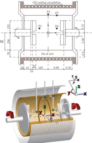
In the VKS2 experiment, the flow cell is enclosed within a layer of sodium at rest!Fig.1". The flow is generated by rotating two impellers with radius of 154.5 mm, 371 mm apart in a thin cylindrical copper vessel, 2R=412 mm in inner diameter, and 524 mm in length. The impellers are
0.75 1.00 0.4 0.30 185 16 206 5 61 78 41 155
Oil cooling circulation
Na at rest P2 P1 x z y 0.90 40 R P4 P3
x
y
z
1
1
2
2
3
3
4
4
5
5
x θ r Px
y
z
FIG. 1.!Color online" Experimental setup. Note the curved impellers, the inner copper cylinder which separates the flow volume from the blanket of surrounding sodium, and the thin annulus in the midplane. Also shown are the holes through which the 3D Hall probes are inserted into the copper vessel for magnetic measurements. Location in !r/R,%,x/R" coordinates of available measurement points: P1!1,!/2,0", P2!1,!/2,0.53",
P3!0.25,!/2,−0.53", P4!0.25,!/2,0.53", and P5!1,!,0" !see TableIfor
details concerning available measurements in different experimental runs". When referring to the coordinates of magnetic field vector B measured in the experiment at these different points, we will use either the Cartesian projection!Bx,By,Bx" on the frame !x,y,z" or the cylindrical projection
!Br,B%,Bx" on the frame !r,%,x" !B%=−Byand Br=Bzfor measurements at
points P1, P2, and P3". We will use in figures the following color code for the magnetic field components: axial!x" in blue, azimuthal !y" in red, and radial!z" in green.
fitted with eight curved blades with height of h=41.2 mm; in most experimental runs, the impellers are rotated so as the blades move in a “nonscooping” direction, defined as the
positive direction by arrows in Fig. 1. The impellers are
driven up to typically 27 Hz by motors with 300 kW avail-able power.
When both impellers rotate at the same frequency F1
=F2, the complete system is symmetric with respect to any
rotation R! of ! around any radial axis in its equatorial
plane !x=0". Otherwise, when F1# F2, the system is not
R!-symmetric anymore. For simplicity, we will also refer to
symmetric/asymmetric system or forcing.
The kinetic and magnetic Reynolds numbers are Re = K2!R2F/&
and
Rm= K"0'2!R2F,
where F=!F1+F2"/2,&is the kinematic viscosity of sodium,
"0is the magnetic permeability of vacuum,'is the electrical conductivity of sodium, and K=0.6 is a coefficient that mea-sures the efficiency of the impellers for exact counter-rotation F1=F2=F.21–23,35 Re can be increased up to 5
(106, and the corresponding maximum magnetic Reynolds
number is Rm=49!at 120 °C". These definitions of Re and
Rm apply to both R!-symmetric and asymmetric forcings,
but the K-prefactor correctly incorporates the efficiency of the forcing only in the symmetric case. Reynolds numbers
may also be constructed either on F1 and F2, e.g., Rm,i
=K"0'2!R2F
i. All these definitions collapse for exact
counter-rotating, i.e., R!-symmetric regimes.
The flow is surrounded by sodium at rest contained in another concentric cylindrical copper vessel, 578 mm in in-ner diameter and 604 mm long. An oil circulation in this thick copper vessel maintains a regulated temperature in the range of 110–160 °C. Note that there are small connections between the inner sodium volume and the outer sodium layer !in order to be able to empty the vessel" so that the outer layer of sodium may be moving; however, given its strong shielding from the driving impellers, we expect its motion to be weak compared to that in the inner volume. Altogether the net volume of sodium in the vessel is 150 l—more details are given in Fig.1.
In the midplane between the impellers, one can attach a thin annulus—inner diameter of 350 mm and thickness of 5 mm. Its use has been motivated by observations in water experiments,21–23,35 showing that its effect on the mean flow is to make the midplane shear layer steadier and sharper. All experiments described here are made with this annulus at-tached; in some cases we will mention the results of experi-ments made without it in order to emphasize its contribution. Finally, one important feature of the VKS2 experiment described here is that the impellers that generate the flow have been machined from pure soft iron !"r&100". One motivation is that self-generation has not been previously observed for identical geometries and stainless steel impel-lers. Several studies have indeed shown that changing the magnetic boundary conditions can change the threshold for
dynamo onset.60,61 In addition, kinematic simulations have
shown that the structure of the sodium flow behind the driv-ing impellers may lead to an increase in the dynamo
thresh-old ranging from 12% to 150%;38 using iron impellers may
protect induction effects in the bulk of the flow from effects occurring behind the impellers. As described in detail below, this last modification allows dynamo threshold to be crossed. We will further discuss the influence of the magnetization of the impellers on its onset.
Magnetic measurements are performed using
three-dimensional!3D" Hall probes and recorded with a National
Instruments PXI digitizer. We use both a single-point!three
components" Bell probe !hereafter labeled G probe" con-nected to its associated gaussmeter and a custom-made array where the 3D magnetic field is sampled at ten locations along a line!hereafter called SM array", every 28 mm. The array is made from Sentron 2SA-1M Hall sensors and is air cooled to keep the sensors’ temperature between 35 and 45 °C. For both probes, the dynamical range is 70 dB, with an ac cutoff at 400 Hz for the gaussmeter and 1 kHz for the custom-made array; signals have been sampled at rates be-tween 1 and 5 kHz.
During runs, we have also recorded other more global data such as torque/power measurements:28,62
!a" The temperature of sodium in the vessel. This is
impor-tant because the electrical conductivity ' of sodium
varies in the temperature range of our experiments. In addition, it gives an alternate way of varying the mag-netic Reynolds number: one may operate at varying speed or varying temperature. We have used
'!T" = 108/!6.225 + 0.0345T" S m−1 !1"
for T!#100,200$ °C.
!b" The torque delivered by the electrical supply of the driving motors. It is estimated from outputs of the UMV4301 Leroy-Sommer generators, which provide an image of the torque fed to the motors and of their velocity!regulated during the runs". We stress that this is an industrial indicator—not calibrated against independent/reference torque measurements.
II. DYNAMO GENERATION, SYMMETRIC DRIVING
F1=F2
A. Self-generation
On September 19th, 2006, we observed the first evidence
of dynamo generation in the VKS experiment.16 The flow
was operated with the thin annulus inserted and the magnetic field was recorded in the midplane using the G-probe located flush with the inner cylinder!location P1 in Fig. 1".
As the rotation rate of the impeller F=F1=F2 is
in-creased from 10 to 22 Hz, the magnetic field recorded by the probe develops strong fluctuations and its main component !in the azimuthal direction at the probe location" grows and saturates to a mean value of about 40 G, as shown in Fig. 2!a". This value is about 100 times larger than the ambient magnetic field in the experimental hall, from which the flow volume is not shielded. The hundred-fold increase is also one order of magnitude larger that the induction effects and field
amplification previously recorded in the VKS experiment with externally applied magnetic field, either homogeneously
over the flow volume19 or localized at the flow boundary.63
We interpret this phenomenon as evidence of dynamo self-generation in VKS2.
The dynamo field is statistically stationary: the compo-nents of the magnetic field measured at the boundary or within the flow display large fluctuations around a nonzero
mean value as seen in Fig. 2. When the experiment is
re-peated, one observes that the azimuthal field at the probe location can grow with either polarity#Fig. 2!b"$ as is ex-pected from the B→−B symmetry of the MHD equations.
The most salient features of this turbulent dynamo have been reported in a letter.16They are given in more detail in this section. We first show that the amplitude of the magnetic field behaves as expected for a supercritical!but imperfect" bifurcation; we discuss the structure of the neutral mode and the influence of the magnetization of the iron impellers. B. Bifurcation
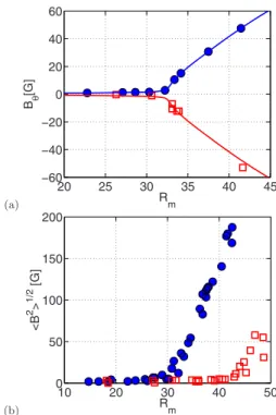
Figure 3!a" shows the evolution of the magnetic field
measured at P1 when the magnetic Reynolds number varies. When Rmexceeds Rmc&32, the magnetic field grows
sponta-neously. In the experiment Rmcan be varied either by
chang-ing the rotation rate of the impellers, or the workchang-ing tempera-ture of the sodium in the vessel, and both effects need to be taken into account when building the bifurcation curves in
Fig.3. In other words, the growth of the magnetic field is
governed by the proximity to threshold in magnetic Rey-nolds number!Rm−Rmc" and not by the single hydrodynamic !rotation rate F" or magnetic !diffusivity 1/"0'" parameters.
The magnetic field grows from very small values !the
induction from the ambient field" and saturates to a value which increases as a function of!Rm−Rmc". The behavior is identical when the magnetic field grows in one direction or the other. In a canonical supercritical bifurcation, one would expect a scaling region Bsat)!Rm−Rmc"a with a=1/2. Our results are compatible with such a behavior, although a better
fit to the data is B%&!Rm−32"0.77 for the azimuthal
compo-nent of the magnetic field!the largest component at the
mea-surement point". More meamea-surements and better statistics will, of course, be needed to get a precise scaling behavior; we also stress that one should proceed with caution when ascribing scaling exponents to this bifurcation. The
instabil-ity grows over a strongly noisy background!the flow
hydro-dynamic turbulence" and no rigorous theory has been devel-oped in this context—the existence of anomalous exponents is an open question.
Another effect that influences the precise shape of the bifurcation is the magnetic behavior of the iron impellers. As
seen in Fig.2, the dynamo field has a strong azimuthal
com-ponent. The iron impellers have a direction of easy magne-tization in the same direction. The coercitivity of pure iron is
weak and the remanent magnetization is of the order of Hc
&100 A/m, while the saturation flux density exceeds
20 000 G. This magnetization of the impellers induces a bias in the dynamo instability. Experimentally we have observed that once the dynamo grows above the onset with a given polarity of the azimuthal field, then it will always start in the same direction when the flow is driven successively below
and above onset. The reverse polarity, as shown in Figs.2
and3, are only observed when the impellers have been
de-magnetized!at least partially" by being exposed to an oscil-latory field. The imperfection induced in the bifurcation is
(a) 10 20 30 40 −60 −40 −20 0 20 Bi ] G[ Bx By Bz 0 10 20 30 40 50 10 15 20 F F ]z H[ time[s] (b) −1000 20 40 60 −50 0 50 100 time [s] B [G] 0 20 40 60 −100 −50 0 50 100 time [s] B [G]
FIG. 2.!Color online" Three components of the magnetic field generated by dynamo action at F1=F2measured at point P1 in the experiment VKS2g.!a"
Growth of the magnetic field as the impellers’ rotation rate F is increased from 10 to 22 Hz.!b" Two independent realizations at same frequency above threshold showing opposite field polarities.
(a) 20 25 30 35 40 45 −60 −40 −20 0 20 40 60 Rm Bθ [G] (b) 10 20 30 40 50 0 50 100 150 200 Rm <B 2 > 1/2 [G]
FIG. 3.!Color online" Bifurcation curves. !a" Azimuthal field measured at P1 for VKS2h, growing with either polarity!only measurements with ini-tially demagnetized impellers are shown here". The solid lines correspond to a best fit with a scaling behavior B%&!Rm−32"0.77 above threshold. !b"
Magnetic field amplitude'B2(1/2=
)
Bx
2+B
y
2+B
z
2at P3 for VKS2i. Impellers
are counter-rotating at equal rotation rates in the positive direction shown in Fig.1!closed blue circles" or in the opposite direction, i.e., with the blades on the impellers moving in a scooping or negative direction !open red squares". Changes in the efficiency of the stirring are taken into account in the definition of Rm; Rm=K"0'R2Fwith K=K+=0.6 in the normal, positive
shown in Fig. 4. The !circles/blue" curve is obtained when starting the experiment from demagnetized impellers and the bifurcation is crossed for the first time. The !squares/red" curve is obtained for further successive variations in the magnetic Reynolds number below and above the onset. As
shown in Ref.64, the rounding off of the bifurcation curve
can be explained in a minimal model for which the magne-tization is coupled to a supercritical bifurcation. Other effects that could be a priori associated with the ferromagnetism of the driving impellers have not been observed. For instance, after the bifurcation has been crossed for the first time, we have not detected any hysteretic behavior of the dynamo onset, and the smooth continuous increase in the field with
!Rm−Rmc" is at odds with the behavior of solid rotor
dynamos.3,4Disk dynamos with imposed velocity would also
saturate to a value directly fixed by the maximum available
mechanical power, in contrast to our observations!cf. Sec.
II E".
One last observation strongly ties the self-generated magnetic field with the hydrodynamics of the flow. Features of the flow!mean geometry and fluctuations" can be changed when the driving impellers are counter-rotated in either di-rection!labeled + or *", or the thin annulus may be inserted
or not in the midplane !called the w and w/o
configurations".22,23,31Bifurcation curves for the +w and −w
cases are shown in Fig.3!b". When the blades of the impel-lers are rotated in “scooping”!*" or nonscooping !+" direc-tions, we note that the dynamo threshold is changed from
F=16 Hz in the +w case to F=18 Hz in the −w/o case, with
corresponding power consumption changing from 40 to 150 kW. Taking into account the change in the efficiency with which the fluid is set into motion, the threshold varies from Rmc=32 to R
m
c&43 in terms of the integral magnetic
Rey-nolds number. For the +w/o case !not shown", the onset is again Rmc&30. However, for the *w/o case we have reached
Rm&49 without observing any dynamo generation. At this
stage a detailed comparison of the hydrodynamics and MHD of the four!+,−,w,w /o" flows is not available, but a water
prototype allows us to measure the ratio+ of the mean
po-loidal velocity to the mean toroidal velocity.21–23,34,35For all
flows, we get +=0.8 except for the !*w/o" flow where +
=0.5. In fact, Ravelet and co-workers22,35showed that for the
VKS2 configuration, +=0.8 is optimal for kinematic
dy-namo, while+=0.5 does not support kinematic dynamo
ac-tion at all. One may suppose that this ratio has an effect on the fully turbulent dynamo action. Furthermore, strong large scale fluctuations of the flow may hinder dynamo action. Such quantities can be evaluated using the ratio,!t" of the instantaneous to the time-averaged kinetic energy densities.31 Within the four considered flows, the!*w/o" flow presents the highest level for both the mean value and the variance of
,!t",31 respectively, 10% and 33% more than the
dynamo-generating flow that fluctuates most!+w/o". C. Geometry of the dynamo field
A central issue is the structure of the magnetic field which is self-sustained above threshold. In order to address it, we have inserted probes and probe arrays at several loca-tions within the sodium flow!cf. Fig.1". Due to our limited sampling in space, we do not fully map the neutral mode; we only obtain indications of its topology. We describe them in detail in this section; measurements reported concern the +w flow case.
In VKS2h runs, simultaneous measurements at points P1 and P5 were performed so that the field is sampled in the midplane at two locations flush with the inner copper
cylin-der and at a !/2 angle. As can be observed in the time
signals shown in Fig.5!a", the azimuthal components of the magnetic fields at these two points vary synchronously. The maximum of the autocorrelation function#Fig.5!b"$ occurs for a zero time lag; its value is less than 0.2 below the dy-namo onset, jumps to 0.5 at the threshold, and saturates to
values around 0.7 for Rmvalues above 36.
In Fig. 5!b", we have plotted times in seconds and ob-serve that all the curves above the dynamo onset almost col-lapse. This behavior persists if time is made nondimensional −100 −5 0 5 10 15 20 20 40 60 80 100 Rm− Rmc B θ [G ]
FIG. 4. !Color online" Bifurcation diagrams measured for the azimuthal component at P1 in VKS2h. The curve with closed blue circles is built when increasing F with demagnetized impellers and crossing the dynamo thresh-old for the first time. Successive cycles in Rmacross the bifurcation
thresh-old all lie on the curve with open red square symbols.
(a) 160 170 180 190 −100 −50 0 time [s] B θ [G] Bθ1 Bθ5 (b) −3 −2 −1 0 1 2 3 0 0.5 1 τ [s] Xcorr(B θ,1 ,B θ,5 ) 44.840.7 36.8 35.6 33.5 31.6 29.8 28.1
FIG. 5. !Color online" Magnetic field measured at points P1 and P5 in VKS2h:!a" Time traces of the azimuthal magnetic field components. !b" Cross correlation function of the two signals for increasing magnetic Rey-nolds numbers in the range of 28–45.
using the diffusion time "0'R2 but does not persist when using the impeller rotation rate F !not shown". This shows that the dynamics is linked to a global magnetic mode rather than controlled by hydrodynamic processes. Another obser-vation is that there is also a strong correlation between the axial and azimuthal components of the magnetic field at a
given location. Figure6shows that its maximum exceeds 0.5
at all Rm, and that it occurs for a time delay increasing with
Rm.
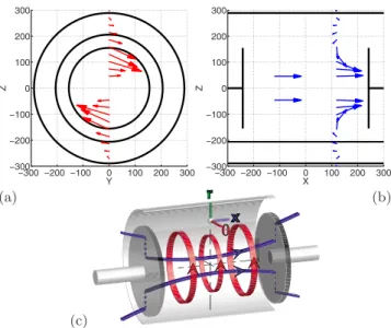
In VKS2i runs, the Hall-probe array was set within the bulk of the flow, nearer to one impeller—point P3. For sev-eral values above onset!Rm=33.9,35.8,41.4", we observe in Fig.7that the normalized field profiles along the array nicely superimpose. Near the rotation axis, the main component is axial; further away the azimuthal component dominates.
Outside of the flow volume!beyond the inner copper
cylin-der" the axial component direction is opposite to that in the center. In the same experiment, the single-point probe was
set nearer to the other impeller!symmetrically with respect
to the midplane, and close to the rotation axis, point P4". The field measured there is mainly axial with the same direction
as at P3. Below threshold, the induction profiles!due to the
presence of the Earth’s field" have the same geometry: the favored dynamo mode is the most efficient with respect to induction.
The combined results of the two sets of experiments are shown in Figs.8!a"and8!b"—the toroidal and poloidal com-ponents are displayed and axisymmetry is assumed. The sim-plest geometry of the magnetic field corresponds to an axi-symmetric field whose axial component has one direction at the center of the cylinder and a reversed direction outside, together with a strong azimuthal component—sketched in Fig.8!c". The dynamo field generated in the VKS2 experi-ment thus involves a strong axial dipolar component. The
determination of its precise geometry !associated higher
modes and their relative amplitudes" needs more precise measurements. However, it strongly differs from the predic-tion of kinematic calculapredic-tions based on the topology of the mean von Kármán flow35,36which tends to favor a transverse
dipole. Invoking Cowling’s theorem,2 the axisymmetric
na-ture of the dynamo fields implies that it has not been gener-ated by the mean flow motions alone. However, an axial dipole is expected for an#-$dynamo. The differential rota-tion in von Kármán flows can generate an azimuthal field from a large scale axial field by torsion of the field lines—the
$effect.65If an # effect takes place, it can produce an azi-muthal current from the aziazi-muthal magnetic field component and, in turn, this current will generate an axial magnetic field. One then has a dynamo loop-back cycle that can
sus-tain an axial dipole. For the # component, several
mecha-nisms have been proposed. For an axisymmetric mean flow, it has been shown that nonaxisymmetric fluctuations can generate such an alpha effect provided that they have no
mirror symmetry.66A scenario was proposed in Ref.64using
the helicity of the flow ejected by the blades of the driving impellers—this flow is nonaxisymmetric with azimuthal wavenumber m=8, helical, and of much larger amplitude and coherence than small scale turbulent fluctuations. In this
−20 −10 0 10 20 −0.2 0 0.2 0.4 0.6 Ω ⋅ τ Xcorr (B x1 ,B θ1 ) 28.1 29.8 31.6 33.5 36.8 40.7 43.8 44.9
FIG. 6.!Color online" Cross correlation function of the axial component and azimuthal component of the field measured inside the flow for increasing magnetic Reynolds numbers in the range of 28–45. Measurements are done at point P1 in VKS2h. 51 79 107 135 163 191 219 247 275 303 −0.3 0.0 0.5 1.0 r [mm] |Bi |/ max (<B θ >) Bx Br Bθ Sodium at rest
FIG. 7. !Color online" Radial profiles of magnetic field. VKS2i measure-ments with the probe array inserted at P3. Measuremeasure-ments for +w flows at
Rm=33.9,35.8,41.4, above the dynamo onset. The magnetic field
compo-nents are normalized by the largest value of the%-component !azimuthal direction": axial !x" is blue, azimuthal !%" is red, and radial !r" is green. The thick vertical line around the seventh sensor!r&211 mm" indicates the position of the inner copper shell; the tenth sensor at r=303 mm is located into the outer copper wall of the vessel.
−300 −200 −100 0 100 200 300 −300 −200 −100 0 100 200 300 Y Z −300 −200 −100 0 100 200 300 −300 −200 −100 0 100 200 300 X Z (a) (b) (c) x x θ r
FIG. 8. !Color online" Geometry of the dynamo mode. The magnetic field amplitudes measured along the probe array in Fig.7is represented by ar-rows:!a" toroidal component, !b" poloidal component, and !c" proposed dipole structure for the neutral mode.
case, an azimuthal loop of magnetic field crosses an array of like-sign helical motions that can induce an azimuthal current.20,67–69Numerical integration of the mean field induc-tion equainduc-tion with an#effect localized in the vicinity of the
impellers70 recently displayed the generation of an axial
magnetic field. The authors of this study thus claim to show
agreement with the scenario proposed in Ref. 64. In mean
field theory,2,71 the most common source of # effect come
from the small scale helicity of turbulence. However, the distribution of helicity in 3D turbulence remains a
challeng-ing question and measurements in model helical flows72,73
have failed to show evidence for this kind of contribution. As
shown by induction measurements in Refs. 72 and 73,
an-other possible contribution to the#effect lies in the spatial inhomogeneity of the turbulence intensity. As shown in Ref.
74, there is a contribution to the mean-field alpha tensor
coming from the inhomogeneity of turbulent fluctuations, with resulting electromotive force-&!g·!"B, where ! is
the flow vorticity and g is the normalized gradient of turbu-lent fluctuations, g=!$u2"/u2. It shows again that an azi-muthal B%field generates a j%current and, therefore, an axial magnetic field. Distinguishing between these mechanisms— which may be linked—will need further measurements, ide-ally from nearby velocity and magnetic probes.
D. Saturation
The amplitude of the magnetic field at saturation is re-lated to the way in which the growing Lorentz forces change the hydrodynamics of the flow. While the value of the thresh-old can be determined by studying the induction equation for a given velocity field—kinematic dynamo simulations—the saturation is governed by nonlinear effects and one must consider the coupled equations of MHD,
%u %t +!u · $"u = − $
*
p . + B2 2"0+
+&/u + 1 ."0!B · $"B, !2" %B %t +!u · $"B = !B · $"u + 1 "0'/B !3"for divergence-free fields. Dimensionally, the value of the magnetic field at saturation can be written as
Bsat=."0V2f!R
m,Pm", !4"
where f is a function of the magnetic Reynolds number Rm
and magnetic Prandtl number Pmand V is some
characteris-tic velocity scale. Functional forms have been determined in limiting cases of laminar and turbulent dynamos.64,75,76In the low!kinetic" Reynolds number limit, the Lorentz force bal-ances the viscous term in the Navier–Stokes equation and one obtains75,76
Bsat2 ) .&
'R2!Rm− Rmc". !5"
In the high magnetic Reynolds number limit, the Lorentz force must be balanced by the nonlinear terms and one gets
Bsat2 ) .
"0'2R2!Rm
− Rmc". !6"
Both possibilities are shown in Fig.9, in which the magnetic Reynolds number has been varied either by changing the rotation rate of the driving impellers or by changing the op-erating temperature and, hence, the sodium’s electrical con-ductivity. Judging from the linearity of the graphs, both seem plausible; however, one may note that the prefactor in the laminar scaling is very large. In other words, a laminar ap-proach, quite doubtful given the high turbulence level in the sodium flow, also underestimates the saturated field by al-most two orders of magnitude. We favor the turbulent scaling and note at this point that the fluctuations play an essential role for the generation of the dynamo and that inertial terms in the Navier–Stokes equation control the nonlinear satura-tion.
E. Power consumption issues
We now turn to the power needed to drive the flow in its steady state, below, or above threshold. Let us call u0!r,t" the velocity field during the linear growth of the dynamo instability, and P0the mechanical power needed to drive this velocity field in a stationary forcing. Given the very high kinetic Reynolds number of the experimental flow, one ex-pects the turbulent scaling P0).L2U03, where L and U0 are characteristic length and velocity scales. We define the
di-(a) 030 32 34 36 38 40 42 50 100 150 (<B> σ R 2/ρν ) 1/2 (b) 30 32 34 36 38 40 42 0 0.1 0.2 0.3 0.4 Rm (<B 2> µ0 σ R 2/ρ ) 1/2
FIG. 9.!Color online" Laminar and turbulent scalings for the magnetic field intensity at saturation. Measurements are shown here for several rotation rates of the impellers and for different operating temperatures T; the mag-netic Reynolds number Rmis rescaled accordingly. Measurement at P1 in
VKS2h,'B2(1/2, =
)
B x 2+B y 2+B z2:!a" laminar scaling #Eq.!5"$ and !b"
turbu-lent scaling#Eq. !6"$. Closed red triangles: F=24 Hz, T=127→143 °C; closed cyan squares: F=19 Hz, T=117→137 °C; open blue circles: F =19 Hz, T=117→145 °C; and open green stars: F=21 Hz, T=124 →152 °C.
mensionless constant !or power number" Kp, using the torques!01,02" or the total power !P0" delivered by the driv-ing motors, as Kp=1 2 01+ 02 .R5!2!F"2= 1 2 P0 .R5!2!F"3, !7"
where we have used R as the characteristic length scale and U0=2!RFas the associated velocity scale. The 1/2 factor in the definition corresponds to the consumption per motor, as used in reports of water-prototype studies.21,22,35Please note that the two formulas in Eq.!7" are only equal because F1
=F2. When a dynamo is generated, the velocity field in the
saturated state is uB!r,t". The mechanical power is now PB and it must feed both the hydrodynamic flow and the mag-netic field: PB= PBhydro+ P
B
mag. The field u
B differs from u0
because the nonlinear saturation has modified the flow. A likely possibility is that the turbulent fluctuations have been changed,64,75–77 and this would also change the mean flow via the Reynolds stress tensor. The power needed in order to sustain the magnetic field must be estimated from
PBmag=
-
j 2 'd 3x=-
!$ ( B"2 "02' d 3x, !8"where j is the current density. With the limited measurements at this stage of the experiment, we cannot resolve indepen-dently PBhydro and P
B
mag, and we can only use the industrial
output of the motors drives as an indicator of P0and PB.
The dimensionless power number is shown in Fig.10for
three sets of experiments. The blue circles correspond to measurements made when driving the flow with stainless steel impellers, a case for which dynamo action was not ob-served. A first observation is that the expected turbulent
scaling—Kp independent of Re or Rm—is observed only for
Rm130 !F116 Hz". The Kp=0.045 value is in agreement
with measurements made in scaled-down water
prototypes.21–23,31 Above Rm=30, some modification must occur because the flow power consumption climbs, in non-dimensional units, from Kp=0.045 to Kp&0.065, when Rm
240 !F224 Hz". This phenomenon, not understood at
present, has to be related to the hydrodynamics of the flow because it is observed in nondynamo experiments. However, for identical rotation rates of the impellers, we measure on average that Kp !dynamo" is typically 10% larger than Kp !nondynamo".
F. Fluctuations
All results presented so far have concerned the average—in time—of the magnetic field recorded by the probes. This section discusses features of the rather large fluctuations about these mean values—as can be seen in Fig. 2. One first observation is that the rms amplitudes in each of the components of the magnetic field increase sharply at
dy-(a) 20 30 40 50 0 5 10 15 20 Rm B θ rms [G] 1st magnetization 2nd magnetization (b) −100 −5 0 5 10 15 5 10 15 20 Rm− Rmc B rms [G] 1st magnetization 2nd magnetization
FIG. 11. !Color online" Evolution with Rmof rms values of the magnetic
field at saturation. Measurements at point P1 in VKS2h.!a" Azimuthal com-ponent B%rms. !b" Magnetic field amplitude Brms. The closed blue circles
corresponds to a first run with almost demagnetized impellers!see text" and the open red squares to the subsequent runs.
10 15 20 25 30 35 40 45 0.15 0.2 0.25 0.3 Rm B rms /<B 2 > 1/ 2
FIG. 12.!Color online" Evolution of the ratio of rms fluctuations to second moment of the magnetic field at point P1.
0 10 20 30 40 50 0.03 0.04 0.05 0.06 0.07 0.08 Rm K p
FIG. 10.!Color online" Evolution with Rmof the power number defined in
Eq.!7"and measured from the drives of the motors. The blue circles!and dashed line as an eye guide" are from nondynamo runs !VKS2f" with stain-less steel impellers. The red stars !VKS2g" and black squares !VKS2h" come from two dynamo runs, with same geometry but with soft-iron impel-lers and also without any magnetic probes in the flow bulk.
namo onset, as shown in Fig.11. This increase defines the same threshold Rmc&32, as estimated from the behavior of the mean values.
Another interesting observation concerns the evolution of the ratio of rms to second moment. It increases very
sharply near onset and then much less rapidly above!cf. Fig.
12". The transition actually allows a determination of the threshold, again at Rmc&32. From a practical point of view, the sharp nonlinear increase in the fluctuations may be a good indicator that one is nearing dynamo onset.
We now study the fluctuations in time of the dynamo field recorded at a fixed location. Each component has in-stantaneous fluctuations that deviate significantly from the
mean values. Figure13 shows the probability density
func-tions!PDFs" for the azimuthal component measured by the
gaussmeter at P1. While sharply peaked about B%=0 below
threshold, the distributions become wide above threshold. At
the highest Rmvalues, one notes the development of a weak
exponential tail to low values with occurrence of events with the reversed polarity. These events, which may also be spa-tially localized within the flow, are not able to reverse the
dynamo. When normalized and centered!inset in Fig. 13",
the distributions are still essentially Gaussian in the vicinity
of the threshold and there is no evidence that the bifurcation proceeds via on “on-off” scenario.55,57–59 Gaussian distribu-tions were also observed for most induction measurements
carried out in the VKS1 setup,19 so that self-excitation has
not induced significant changes in behavior here—in
agree-ment with measureagree-ments in the Karlsruhe dynamo.10
The fluctuations whose statistics are given above occur over a wide range of time scales. The time spectra give the distribution of energy among these scales. Since the fluctua-tions of the magnetic field measured at a given location in the experiment are expected to be sensitive to the local tur-bulence intensity, we discuss in the following the magnetic energy spectra measured at different locations and at differ-ent magnetic Reynolds numbers.
We report in Fig. 14 the magnetic spectra measured
above the dynamo threshold at different distances from the axis of the experiment along a radius passing through point P3. We observe a clear dependence of the global shape of the spectra depending on the location. The spectra exhibit ranges to which one may want to ascribe traditional turbulence scal-ing behavior:
!a" For f 3F/10, the spectra are essentially flat; note
how-ever a broad frequency peak around flow&F/10 !we
will see further that flow&0.14F".
!b" In the range F/103 f 34F, the spectra are consistent
with power laws: f−1 for the azimuthal and the radial
components and f−5/3for the axial component.
!c" At larger frequencies, the magnetic energy decays rap-idly within a short range!4F3 f 38F" possibly consis-tent with a f−11/3decay, also known to exist in numer-ous induction experiments with liquid metals19,65 and
an even steeper decay !close to f−6" at larger
frequencies.
As we study signals from sensors at increasing radial distances from the axis, these regimes disappear. Harmonics locked to the impellers’ rotation rate become visible: har-monic 8 is particularly intense for sensors at r3215 mm, inside the inner copper vessel. This is very likely to be re-lated to the fact that the impellers are fitted with eight blades and that those sensors intercept the centrifugal flow ejected at the periphery by the blades. As we move into the layer
with sodium at rest !r4210 mm", the global energy of the
−150 −100 −50 0 50 10−4 10−2 100 Bθ [G] PDF 28.1 29.8 31.6 33.5 36.8 40.7 44.9 −5 0 5 10−4 10−3 10−2 10−1 100 (B − <B >)/Brms θ θ θ PDF
FIG. 13.!Color online" PDFs of local fluctuations of B%. Measurement at
point P1, VKS2h. Magnetic Reynolds numbers are given in the legend and profiles below onset cannot be distinguished. Inset: PDFs for centered and normalized variables. 100 101 102 103 10−6 10−4 10−2 100 102 f (Hz) Sp(B r ) r=46 mm r=102 mm r=158 mm r=214 mm r=270 mm f−1 f−11/3 100 101 102 103 10−6 10−4 10−2 100 102 f (Hz) Sp(B θ ) r=46 mm r=102 mm r=158 mm r=214 mm r=270 mm f−1 f−11/3 100 101 102 103 10−6 10−4 10−2 100 102 f (Hz) Sp(B x ) r=46 mm r=102 mm r=158 mm r=214 mm r=270 mm f−5/3 f−11/3 (a) (b) (c)
FIG. 14.!Color online" Time spectra of magnetic field fluctuations measured with the probe array at point P3 !location of the innermost sensor" in VKS2i. Different curves on each plot correspond to different sensor depth, labeled in the legend by their distance r to the rotation axis. The rotation frequency of the impellers is 20 Hz:!a" Axial component, !b" azimuthal component, and !c" radial component.
fluctuations significantly decreases; a decay due to the pres-ence of ohmic dissipation remains visible as well as the first harmonics of the impellers’ rotation rate.
We now discuss the evolution of spectra with Rm,
mea-sured at the innermost location within the flow!Fig.15". The different power law regimes remain, with their exponents unchanged for all values of the magnetic Reynolds number. We find that the transition between the different regimes is locked to forcing frequency F. The low frequency peak is systematically present and centered around flow&0.14F
re-gardless of the Reynolds number. The f−1 regime, which
re-mains present for the azimuthal and radial component, may
be interpreted as 1/ f noise due to the presence of several
characteristic time scales in the flow. At larger frequencies, above the magnetic diffusion cutoff, the f−11/3 regime is ex-pected, under a Taylor hypothesis, from the balance in the induction equation between the magnetic induction term— with a fully turbulent velocity field—and the Ohmic dissipa-tion term. The shortness of the f−11/3regime that we observe and the steeper decrease observed above the eighth harmonic can be attributed to a spatial filtering due to the dimension l0&3 cm of the tube containing the probe. The spatial inte-gration of magnetic fluctuations at the scale l0attenuates the spatial magnetic spectra by a factor k−2, which under a Tay-lor hypothesis, should lead in the frequency spectral domain to a f−17/3& f−5.7regime consistent with the steep energy de-crease measured for large frequencies fluctuations. In this scenario the cutoff frequency between the f−11/3and the f−17/3 regimes is proportional to l0v, with v the characteristic local
velocity at the probe location. This is consistent with the observation that the transition is locked to the impellers’ ro-tation rate.
Finally, we discuss measurements taken in the midplane, flush with the lateral wall, which have different
characteris-tics. Figure 16 shows the evolution of spectra as the
mag-netic Reynolds number is increased. The three components have a similar behavior #Fig.16!a"$. One notes a net mag-netic energy increase as the dynamo threshold is crossed. At all magnetic Reynolds number, the spectra exhibit a low
fre-quency peak flow&0.14F and a peak at a frequency
corre-sponding to the rotation rate of the impellers, also present in the measurements at points P3 and P4 previously discussed. Although the evidence of power law dependence of the spec-trum is again restricted to relatively short ranges, different regimes may be identified:
!a" At low frequencies !typically f 3 flow" a slow decay
with an exponent #1 changing from #1&0 below
threshold to#1&−0.5 above threshold.
!b" At intermediate frequencies !typically flow3f 3F" the
energy decay is faster with an exponent #2, changing
from #2&−2 below threshold to #2&−2.5 above
threshold.
!c" In the high frequency range !typically f 4F", as shown in the semilog representation in Fig.16!c", the spectra are better described by an exponential decay exp!−f/ fexp". We find that fexpis of the order of 1.4F.
III. DYNAMICAL REGIMES WITH ASYMMETRIC FORCING F1ÅF2
A. Asymmetric flow forcing
In this section, we report results obtained when the im-pellers rotate at different frequencies!F1# F2". Different sets of parameters can be used to describe these forcing configu-rations:!i" F1 and F2, the two impellers frequencies;!ii" F =!F1+F2"/2 the mean frequency and
5=!F1− F2"/!F1+ F2"
the nondimensional difference; and!iii" any other combina-tions of F1and F2. In a half-scale water model experiment, it
has been shown from torque measurements21 that there are
strong similarities between the von Kármán flow forced by
10−2 10−1 100 101 10−4 10−2 100 102 f⋅ F−1 Sp(B x ) Rm=29.9 Rm=31.7 Rm=34.7 Rm=38.4 f−5/3 f−11/3 f−17/3 10−2 10−1 100 101 10−4 10−2 100 102 f⋅ F−1 Sp(B r ) Rm=29.9 Rm=31.7 Rm=34.7 Rm=38.4 f−1 f−11/3 f−17/3 (a) (b)
FIG. 15. !Color online" Time spectra of magnetic field fluctuations mea-sured for different values of Rmat point P4 during VKS2i:!a" axial
compo-nent and!b" radial component.
10−2 10−1 100 101 10−6 10−4 10−2 100 102 f F−1 Sp(B x1 ),Sp(B y1 ),Sp(B z1 ) Bx1 By1 Bz1 10−2 10−1 100 101 10−6 10−4 10−2 100 102 f F−1 Sp( B x1 ) 28.0946 29.78 31.588 33.5311 36.8452 40.7409 43.7982 44.9551 0 5 10 15 20 10−6 10−4 10−2 100 102 f F−1 Sp( Bx1 ) 28.0946 29.78 31.588 33.5311 36.8452 40.7409 43.7982 44.9551 (a) (b) (c)
FIG. 16.!Color online" Time spectra of magnetic field fluctuations at point P1. !a" Three components, Rm&40; #!b" and !c"$ log-log plot and semilog plots
impellers rotating respectively at F1and F2in the laboratory frame or by impellers rotating at!F1+F2"/2 in a frame ro-tating at!F1−F2"/2. More recently, stereoscopic particle
im-age velocimetry measurements have confirmed this finding.23
It is thus convenient to choose F and 5 as control parameters since F appears as the effective forcing shear in the rotating
frame and,5, measures the relative importance of the global
rotation to shear.
These asymmetric regimes have been studied in water experiments allowing a good understanding of the hydrody-namic bifurcations of the flow when breaking the forcing symmetry.21,22,78 When increasing or decreasing one of the impeller rotation rates from a symmetric configuration, the cell closer to the fastest impeller grows in size and the shear layer is translated toward the slowest impeller. When only one impeller rotates, the flow is made of one single pumping cell rotating with the stirring impeller—similar to the s1t1
flow.32The evolution between these extreme cases!generally
referred to as the “turbulent bifurcation”" depends on the impeller and vessel geometry: In some cases, the transition
between the two extreme flow topologies !two symmetric
cells versus one single cell" is smooth and continuous, but it might also be sudden,31,78leading to first order transitions in
any order parameter chosen to describe it !average position
of the shear layer, torque delivered by the motors, etc.".
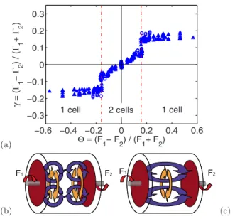
Figure17shows the evolution of the reduced
dimension-less torques
6=!01− 02"/!01+ 02"
delivered by the motors as a function of 5. One can see the
sudden transition for,5,=5c%0.16, corresponding, e.g., to
F1=22 Hz and F2%15.8 Hz. At this point the flow transits
between one-cell and two-cell topologies.22,31,78 The transi-tions are very sharp and the corresponding hysteresis do-mains are very narrow.
B. A variety of regimes
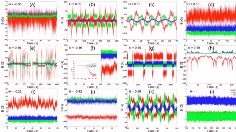
We first report observations of dynamo regimes when varying the frequency of rotation of the impellers. Not all
possible combinations have been explored—Fig.18
summa-rizes the visited regions of parameter space. They are plotted in terms of the experimental control parameters!F1,F2" and also as a function of the differential rotation 5 and of an average magnetic Reynolds number based on the global ro-tation rate F=!F1+F2"/2. In Fig. 18!b", symmetry between the positive and negative values of 5 has been assumed and observed dynamical regimes will be discussed according to
this hypothesis, with F and,5, being the control parameters.
For Rm!F"&35, and for increasing ,5,, one gets
successively—Fig.18!b"—the following main regimes:
!1" Stat1: ,5,10.09; stationary dynamos of the same type as observed for the symmetric 5=0 forcing. An ex-ample of time trace of the three components of magnetic field measured at P1 is shown in Fig.19!a".
!2" Limit cycle!LC":,5,&0.1; for several time-periodic
re-gimes between the Stat1 and Stat2 states #Figs. 19!b"
and19!c"$. These regimes have been studied in detail in Ref.18. (a) −0.6 −0.4 −0.2 0 0.2 0.4 0.6 −0.3 −0.2 −0.1 0 0.1 0.2 0.3 Θ = (F1− F2) / (F1+ F2) γ =( Γ 1 − Γ 2 )/( Γ 1 + Γ 2 )
1 cell 2 cells 1 cell
(b)
F2
F1 F1 F2
(c)
FIG. 17. !Color online" !a" Measurement of the reduced dimensionless torque 6=!01−02"/!01+02" vs 5=!F1−F2"/!F1+F2". Data are from
VKS2g!open circles" and VKS2h !closed triangles", i.e., without probes in the flow bulk which strongly affect6in the one-cell regimes. Data have been symmetrized.!b" Schematic configuration of the mean flow in the two-cell regime for small 5!F1%F2", as measured in water. !c" Schematic
configuration of the mean flow in the one-cell regime for large 5!F17F2".
0 10 20 30 40 50 60 0 10 20 30 40 50 60 Rm,1 R m,2 0 0.1 0.2 0.3 0.4 0.5 0.6 0.7 0.8 0.9 1 0 10 20 30 40 50 |Θ| = (F1− F2)/(F1+ F2) R m [(F 1 +F 2 )/2]
STAT1 STAT2 STAT3 OSCILLATIONS STAT4
LIMIT
CYCLEREV. BURSTSEXTINCT.
no dynamo STAT1 STAT2 STAT3 STAT4 extinction reversals oscillation limit cycle bursts (a) (b)
FIG. 18.!Color online" Parameter space and dynamo regimes for VKS2g, VKS2h, and VKS2i. !a" In the !Rm,1,Rm,2" plane. !b" In the #Rm!F",,5,$ plane, i.e.,
!3" Stat2: 0.111,5,10.13; stationary regimes #Fig.19!d"$.
!4" Reversal: ,5,!#0.15–0.18$; reversing dynamos17,18
#Fig.19!g"$.
!5" Bursts–ext: ,5,&0.2; regimes with a “bursting” dynamo field where the magnetic field has on average a low value with sudden “jerks” to much larger intensities #Figs.19!e"and19!h"$. In this region we have also ob-served cases where dynamo action was not obob-served within 3 minutes test periods, as well as cases when an initial dynamo decays to zero. They have been called “extinctions”#Figs.19!f"and25!d"$.
!6" Stat3: 0.21,5,10.4; stationary dynamos #shown in Figs.19!i"and19!j"$.
!7" Osc: ,5,20.4; oscillatory dynamos. When increasing further the rotation component of the forcing, oscillatory dynamos are starting from the Stat3 stationary ones. An example is given in Figs.19!k"and27!a".
!8" Stat4: at ,5,=1, when the flow is driven by the rotation of only one impeller, one observes an abrupt bifurcation
to a stationary dynamo of very low !finite" amplitude
#Fig. 19!l"$. Note that intermediate forcing conditions !0.63,5,11" are not reachable at present for mechani-cal reasons.
We note that at Rm!F"%35 a dynamo is always
gener-ated for all explored values of 5. 5 thus plays an important role in the selection of the dynamo regime; it does not choose it uniquely as we have observed in several cases that the dynamo at given values of!F1,F2" depends on the path that has been followed.
C. Stationary dynamo regimes, "Å0
Although a variety of dynamical regimes have been ob-served when the flow is driven with impellers counter-rotating at different rates, a large fraction of the phase space is actually populated by stationary regimes!see Fig. 18". In future studies these regimes will need to be fully character-ized in terms of mode geometry, type of dynamo bifurcation, etc. For the moment, we classify them in broad classes sepa-rated by time-dependent dynamos and consider the three cases for,5,30.6. The first one #Stat1; Fig.19!a"shows a typical time series, see also Fig.2$ appears at low values of 5 !,5,10.09". The second regime #Stat2; Fig. 19!d"$
ap-pears as one increases 5 !0.111,5,10.13", but it is
sepa-rated from the first by a small range of 5 with a reversing regime. The third stationary regime #Stat3; Fig. 19!j"$
ap-pears at larger values of 5 !0.21,5,10.4". The main
dif-ference can be observed in the fluctuations, which are domi-nated by very slow oscillations, with periods of several seconds. This observation is confirmed in Fig.20!a", show-ing the power spectrum density for the three stationary re-gimes. Note that the three spectra collapse when the fre-quency is rescaled by the mean rotation frefre-quency of the impellers, F=!F1+F2"/2, at least for the frequencies larger than F. The small scale fluctuations in the spectrum are thus set by the effective Rm, i.e., turbulence. In Fig. 20!b", the centered and normalized PDFs of the three regimes are pre-sented and display a fairly Gaussian behavior, like in the case of exact counter-rotation!see Fig.13".
FIG. 19.!Color online" Examples of observed dynamo regimes for increasing values of ,5,. See text for details. Color code #see caption of Fig.1and legend of Fig.2!a"$ for the magnetic field components: axial !x" in blue, azimuthal !y" in red, and radial !z" in green.
Although we have not systematically mapped the
!Rm,5" plane, some observations can be made about the
dynamo bifurcation in these regimes. For the Stat1 regime, the bifurcation seems supercritical with a threshold around
Rm=31, similar to the counter-rotating case, but the
depen-dence of the threshold on 5 has not been precisely deter-mined. However as one proceeds to more asymmetric re-gimes, in the case of Stat2 and Stat3, the dependence of the
dynamo field on the value of 5, as well as Rm, is more
pronounced. A hysteretic behavior takes place, where the value of the magnetic field at saturation depends on the path followed.
In the limit of the flow being driven by the rotation of a single impeller!the other being kept at rest, i.e., 5= 81", we observe an abrupt bifurcation to stationary dynamo Stat4. As the rotation rate of the impeller is increased above threshold, the amplitude of the magnetic field increases slightly to reach
a maximum at Rm=23 Hz, then decreases to almost zero at
the maximum rotation rate!Rm=26". Such Rmdecrease in the dynamo is also observed when the equatorial annulus is re-moved but then the stationary regime exchanges stability with an oscillatory regime, with a bistability region.79 D. Reversals
Decreasing the frequency of one impeller from the
sta-tionary dynamo regime at F1=F2=22 Hz, we performed the
first observation of reversals of the magnetic field in a fluid dynamo.17These reversals at irregular time intervals are
dis-played in Fig.21for a sensor located at point P2. For each
polarity, either positive or negative, the amplitude of the magnetic field has strong fluctuations, with a rms fluctuation level of the order of 20% of the mean. This level of fluctua-tion is due to the very intense turbulence of the flow, as the
kinetic Reynolds number exceeds 106. Reversals occur
ran-domly and have been followed for up to 45 min, i.e., 54 000 characteristic time scales of the flow forcing.
The polarities do not have the same probability of obser-vation. Phases with a positive polarity for the largest mag-netic field component have, on average, longer duration !'T+(=120 s" than phases with the opposite polarity !'T−( =50 s". This asymmetry can be due to the ambient magnetic field. Note however that the amplitude of the magnetic field
is the same for both polarities. Standard deviations are of the same order of magnitude as the mean values, although better statistics may be needed to make these estimates more pre-cise. The mean duration of each reversal,9&5 s, is longer than MHD time scales: the flow integral time scale is of the order of the inverse of the rotation frequencies, i.e., 0.05 s, and the Ohmic diffusive time scale is roughly9:&0.4 s.
When the amplitude of the magnetic field starts to decay, either a reversal occurs, or the magnetic field grows again with its direction unchanged. Similar sequences, called ex-cursions or aborted reversals,80,81 are observed in recordings of the Earth’s magnetic field. We have also observed that the trajectories connecting the symmetric states B and −B are quite robust despite the strong turbulent fluctuations of the flow. This is displayed in Fig.21!a": the time evolution of reversals from positive to negative states can be neatly su-perimposed by shifting the origin of time such that B!t=0" =0 for each reversal. Despite the asymmetry due to the Earth’s magnetic field, negative-positive reversals can be su-perimposed in a similar way on positive-negative ones if −B is plotted instead of B. For each reversal the amplitude of the field first decays exponentially. A decay rate of roughly 0.8 s−1 is obtained with a log-linear plot!not shown". After changing polarity, the field amplitude increases linearly and then displays an overshoot before reaching its statistically stationary state. The signal thus clearly breaks the time re-versal symmetry, a common feature for many relaxation os-cillations or heteroclinic cycles in low dimensional dynami-cal systems. A similar asymmetry in time, with a slow decay of the field amplitude followed by a fast recovery after changing sign, has been reported in recordings of the Earth magnetic field.82
Magnetic field reversals have been found in the same
region of parameter space during all the runs !VKS2g,
VKS2h, and VKS2i". The characteristics described above have been found reproducible except the nearly perfect su-perimposition displayed in Fig. 21!VKS2g". In the follow-ing runs where measurements were performed at P1 and P3, although a most probable trajectory clearly appears, some reversals follow a significantly different one between 8B.
10−2 10−1 100 101 10−2 100 102 104 106 f F−1 PSD STAT1 STAT2 STAT3 −6 −4 −2 0 2 4 6 10−5 10−4 10−3 10−2 10−1 (By−<By>)/std(By) PDF STAT1 STAT2 STAT3 gaussian (a) (b)
FIG. 20.!Color online" !a" Power spectrum density. Frequency is normal-ized by the average frequency of the impellers F=!F1+F2"/2. The dashed
line shows the *1 slope as a guide for the eye.!b" Centered PDF, normal-ized by its rms value. Quantities are computed from the azimuthal compo-nent in the time signal in Fig.19for the regimes Stat1, Stat2, and Stat3.
0 200 400 600 800 −200 0 200 Time [s] B i [G] −5 0 5 10 Time [s] (a) (b)
FIG. 21.!Color online" Reversals of the magnetic field generated by driving the flow with counter-rotating impellers at frequencies F1=16 Hz and F2
=22 Hz!5=0.16, VKS2g". !a" Time recording of the three magnetic field components at P2: axial!x" in blue, azimuthal !y" in red, and radial !z" in green#see legend of Fig.2!a"$. !b" superimposition of the azimuthal com-ponent for successive reversals from negative to positive polarity together with successive reversals from positive to negative polarity with the trans-formation B→−B. For each of them the origin of time has been shifted such that it corresponds to B=0.