HAL Id: cea-02157026
https://hal-cea.archives-ouvertes.fr/cea-02157026
Submitted on 14 Jun 2019
HAL is a multi-disciplinary open access
archive for the deposit and dissemination of
sci-entific research documents, whether they are
pub-lished or not. The documents may come from
teaching and research institutions in France or
abroad, or from public or private research centers.
L’archive ouverte pluridisciplinaire HAL, est
destinée au dépôt et à la diffusion de documents
scientifiques de niveau recherche, publiés ou non,
émanant des établissements d’enseignement et de
recherche français ou étrangers, des laboratoires
publics ou privés.
How the power spectrum of dust continuum images may
hide the presence of a characteristic filament width
A. Roy, Ph. André, D. Arzoumanian, M.-A. Miville-Deschênes, V. Könyves,
N. Schneider, S. Pezzuto, P. Palmeirim, J. M. Kirk
To cite this version:
A. Roy, Ph. André, D. Arzoumanian, M.-A. Miville-Deschênes, V. Könyves, et al.. How the power
spectrum of dust continuum images may hide the presence of a characteristic filament width.
As-tronomy and Astrophysics - A&A, EDP Sciences, 2019, 626, pp.A76. �10.1051/0004-6361/201832869�.
�cea-02157026�
c
ESO 2019
Astrophysics
&
How the power spectrum of dust continuum images may hide the
presence of a characteristic filament width
A. Roy
1,2, Ph. André
1, D. Arzoumanian
3, M.-A. Miville-Deschênes
1,4, V. Könyves
1, N. Schneider
5,
S. Pezzuto
6, P. Palmeirim
7, and J. M. Kirk
81 Laboratoire d’Astrophysique (AIM), CEA, CNRS, Université Paris-Saclay, Université Paris Diderot, Sorbonne Paris Cité,
91191 Gif-sur-Yvette, France
e-mail: aroy@cita.utoronto.ca, pandre@cea.fr
2 Laboratoire d’Astrophysique de Bordeaux, Univ. Bordeaux, CNRS, B18N, Allée G. Saint-Hilaire, 33615 Pessac, France 3 Department of Physics, Nagoya University, Furo-cho, Chikusa-ku, Nagoya, Aichi 464-8602, Japan
4 Institut d’Astrophysique Spatiale, CNRS, Univ. Paris-Sud, Université Paris-Saclay, Bâtiment 121, 91405 Orsay Cedex, France 5 I. Physik. Institut, University of Cologne, Zülpicher Str. 77, 50937 Koeln, Germany
6 INAF – Istituto di Astrofisica e Planetologia Spaziali, Via Fosso del Cavaliere 100, 00133 Roma, Italy
7 Instituto de Astrofísica e Ciências do Espaço, Universidade do Porto, CAUP, Rua das Estrelas, 4150-762 Porto, Portugal 8 University of Central Lancashire, Preston, Lancashire PR1 2HE, UK
Received 21 February 2018/ Accepted 26 March 2019
ABSTRACT
Context. Herschel observations of interstellar clouds support a paradigm for star formation in which molecular filaments play a cen-tral role. One of the foundations of this paradigm is the finding, based on detailed studies of the transverse column density profiles observed with Herschel, that nearby molecular filaments share a common inner width of ∼0.1 pc. The existence of a characteristic filament width has been recently questioned, however, on the grounds that it seems inconsistent with the scale-free nature of the power spectrum of interstellar cloud images.
Aims. In an effort to clarify the origin of this apparent discrepancy, we examined the power spectra of the Herschel/SPIRE 250 µm images of the Polaris, Aquila, and Taurus–L1495 clouds in detail and performed a number of simple numerical experiments by inject-ing synthetic filaments in both the Herschel images and synthetic background images.
Methods. We constructed several populations of synthetic filaments of 0.1 pc width with realistic area filling factors (Afil) and
distri-butions of column density contrasts (δc). After adding synthetic filaments to the original Herschel images, we recomputed the image
power spectra and compared the results with the original, essentially scale-free power spectra. We used the χ2
varianceof the residuals
between the best power-law fit and the output power spectrum in each simulation as a diagnostic of the presence (or absence) of a significant departure from a scale-free power spectrum.
Results. We find that χ2
variancedepends primarily on the combined parameter δ 2
cAfil. According to our numerical experiments, a
sig-nificant departure from a scale-free behavior and thus the presence of a characteristic filament width become detectable in the power spectrum when δ2
cAfil' 0.1 for synthetic filaments with Gaussian profiles and δ2cAfil' 0.4 for synthetic filaments with Plummer-like
density profiles. Analysis of the real Herschel 250 µm data suggests that δ2
cAfilis ∼0.01 in the case of the Polaris cloud and ∼0.016 in
the Aquila cloud, significantly below the fiducial detection limit of δ2
cAfil ∼ 0.1 in both cases. In both clouds, the observed filament
contrasts and area filling factors are such that the filamentary structure contributes only ∼1/5 of the power in the image power spec-trum at angular frequencies where an effect of the characteristic filament width is expected.
Conclusions. We conclude that the essentially scale-free power spectra of Herschel images remain consistent with the existence of a characteristic filament width ∼0.1 pc and do not invalidate the conclusions drawn from studies of the filament profiles.
Key words. local insterstellar matter – submillimeter: ISM – stars: low-mass – infrared: diffuse background
1. Introduction
Recent Herschel imaging observations of nearby molecular clouds, for example, those obtained as part of the Herschel Gould Belt Survey (HGBS; André et al. 2010), indicate that filamentary structures are characterized by a common inner width Wfil ∼ 0.1 pc, with only a factor of approximately two
spread around this value, over a wide range of column densities (Arzoumanian et al. 2011,2019;Koch & Rosolowsky 2015). If confirmed, the existence of such a characteristic filament width has remarkable implications for the star formation process and is one of the bases of a proposed filamentary paradigm for solar-type star formation (André et al. 2014). In particular, it may set a critical column density threshold above which most
stars form in filamentary molecular clouds. For filaments of ∼0.1 pc width and a typical gas temperature of 10 K, the criti-cal mass per unit length Mline,crit = 2 c2s/G ∼ 16 M pc−1 (cf.
Inutsuka & Miyama 1997) indeed translates to a critical col-umn density Σgas,crit ∼ Mline,crit/Wfil ∼ 160 M pc−2, which is
close to the background column density threshold above which prestellar cores are found with Herschel in nearby regions (e.g., Könyves et al. 2015; Marsh et al. 2016). Above this threshold, the star formation rate is observed to be directly proportional to the mass of dense molecular gas in both nearby clouds and exter-nal galaxies (e.g.,Gao & Solomon 2004;Heiderman et al. 2010; Lada et al. 2010;Shimajiri et al. 2017).
Arzoumanian et al. (2011) suggested the existence of a characteristic filament width after fitting simple Gaussian or
Plummer-like model profiles to the transverse profiles observed with Herschel for a broad sample of nearby filaments (see also Arzoumanian et al. 2019). In the analysis of Arzoumanian et al., thermally supercritical filaments (with Mline > 2c2s/G) tend to
have Plummer-like density profiles with a flat inner region of radius Rflat and a decreasing power-law wing ρ ∝ r−2 at larger
radii. In contrast, low column density, thermally subcritical filaments (with Mline < 2c2s/G) tend to be better described by
Gaussian density profiles.
Why molecular filaments seem to share such a char-acteristic width is still a debated theoretical problem (e.g., Hennebelle & André 2013; Fischera & Martin 2012; Federrath 2016;Auddy et al. 2016). In order to ascertain whether the pres-ence of this possibly universal filament scale is robust, the obser-vational data also need to be investigated using various other means. In a recent paper,Panopoulou et al.(2017) tested the pos-sibility of identifying a characteristic scale using a power spec-trum analysis. In their study they argued that, had there been a characteristic filament width, its signature should have mani-fested itself in the power spectrum of Herschel images of nearby clouds, either as a kink or as a change in slope at an angular frequency corresponding to the characteristic scale.
In the present paper, we revisit the latter issue from an observer’s standpoint, exploring the parameter space with real-istic filament properties consistent with the observational data, in particular taking into account realistic distributions of fila-ment contrasts and area filling factors. To this end, we selected two extreme regions imaged by the HGBS, namely the Polaris translucent cloud, mainly dominated by low density subcritical (Mline < Mline,crit) filaments, and the Aquila complex, which
contains a fair population of high column density supercritical (Mline > Mline,crit) filaments. We also used the B211/B213 field
in the Taurus cloud, which is dominated by a single, marginally supercritical filament.
The layout of the paper is as follows. In Sect.2we describe the construction of synthetic filament images and their power spectra. In Sect. 3, we develop a diagnostic for the detection of a characteristic filament width in a power spectrum plot. We also develop a diagnostic for the detection of a characteristic fil-ament width in a power spectrum plot. In Sects.4and5, we per-form a power spectrum analysis of the Herschel images of the Polaris and Aquila clouds, respectively, and compare the results to those obtained on synthetic maps after adding simulated filaments. In Sect. 6, we compared power spectra of a subre-gion of Taurus molecular cloud encompassing the Taurus main filament to a synthetic filament with similar physical properties as B211/B213. In Sect.7, we investigate the combined effect of filament column density contrast (δc) and area filling factor (Afil).
Finally, we summarize our results in Sect.8.
2. Construction of synthetic filaments and their power spectra
Figure 1 shows an example of a synthetic filament with a transverse Gaussian profile and a projected spatial inner width (FWHM) of 0.1 pc at a distance of 140 pc. Mathematically, the 2D image of a filament with a Gaussian profile can be expressed as
ICylinder(x, y)= C hδL(ax+ by + c) × ΠLi ? Gθfil(x, y), (1)
where, C is the amplitude factor (related to the filament contrast) of the delta line function δL(ax+ by + c), ΠLis a rectangle
func-tion, and the ? symbol denotes the convolution operator. The
Fig. 1.Image of a simulated filament with a Gaussian transverse profile
and a FWHM width of 0.1 pc, projected at a distance of 140 pc. Here, the level of filament contrast was adjusted so that δc∼ 10.
delta line function assumes a value of unity when its parameter ax+by+c = 0, and zero elsewhere. The expression ax+by+c = 0 is the equation of a straight line where the a, b coefficients deter-mine the slope of the straight line and c is the intercept. The rect-angle function,ΠL, which has a value of unity over the length L
of the line function and zero elsewhere, transforms the line into a line-segment of length L. In order to make a Gaussian filament profile, we convolve the entire line segment [δ(ax+ by + c) × ΠL]
with a Gaussian kernel, Gθfil(x, y), of full width at half maximum
FW H M= θfil.
The FWHM of the Gaussian kernel= θfilis chosen such that
the projected spatial width is Wfil. To create a characteristic Wfil
inner width of a filament at a distance d, the required θfilis
θfil' 14700× Wfil 0.1 pc ! × 140 pc d ! · (2)
The choice of the parameter C depends upon the required level of filament contrast defined as δc = (Ipeak− Ibkg)/Ibkgand
on the dilution factor of the convolution kernel,
C ≈δcθfil. (3)
For example, in order to create a Gaussian filament profile of spatial FW H M= 0.1 pc and contrast δc= 0.4 at the distance of
Polaris (d= 140 pc,Falgarone et al. 1998), we used a Gaussian convolution kernel of θfil ∼ 14700 (see Eq. (3)), and a contrast
amplitude of C ∼ 0.4 × 14700/θ
pix, where θpixis the pixel size of
the image. We adopted a pixel size θpix= 600for Herschel/SPIRE
250 µm images (18.200beam resolution).
The Fourier transform of a 2D image can be expressed as ˆI(kx, ky)=
Z
I(x, y)e−2πi(kxx+kyy)dx dy, (4)
where dx dy is the infinitesimal surface area, andR dx dy = S is the total surface area, S , covered by the map. For an image of a single cylindrical filament, most of the contribution to the integral in Eq. (4) comes from integration over the central part of the filament which encloses 75% of the total intensity fluctuations.
The power spectrum of a cylindrical intensity distribution can be written analytically as
Pcylinder(kx, ky)= | ˆI(kx, ky)|2,
= |FT(δL(ax+ by + c)(k
x, ky)|2Gˆ2(kx, ky),
= |ˆδ(bkx− aky)|2Gˆ2(kx, ky), (5)
where ˆδ(bkx− aky) is the Fourier transform of the delta line
func-tion δL(ax+ by + c) and ˆG(kx, ky) is the Fourier transform of the
convolution kernel. The power spectrum of the Gaussian kernel, ˆ
G2(kx, ky), is also a Gaussian, and its FWHM widthΓfilis related
to the FWHM width θfilof Gθfil(x, y) through the relation:
Γfil=
√
8ln2/πθfil
∼ 0.6/θfil. (6)
One may thus expect a characteristic filament width θfil to
lead to a signature in the power spectrum at angular frequencies kfil∼Γfil.
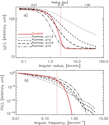
For multiple, randomly distributed filaments, as in the sim-ulations discussed below, it is not possible to obtain the power spectrum analytically. We therefore used the IDL-based routine FFT to compute the power spectrum. Nevertheless, Eq. (5) is useful to appreciate how the power spectrum of an image with a single filament is dominated by the power spectrum of the con-volution kernel. As an illustration, Fig. 2b displays the power spectra of images including a single model filament with either a Gaussian or a Plummer-like density profile. The red curve in Fig. 2a shows the radial profile of the Gaussian filament dis-played in Fig.1. The over-plotted black curves show the profiles of filaments featuring Plummer-like power-law wings at large radii, with power-law slopes ranging from p= 1.5 to p = 4. The flat inner region of each Plummer-like model filament had a con-stant Rflatof ∼0.03 pc. An example of filament with a transverse
Plummer profile is shown in Fig. A.1. Figure2b displays the power spectra corresponding to the filament profiles shown in Fig.2a. At high angular frequencies, the power decreases expo-nentially following the same trend as the power spectrum of the convolution kernel. An example of a filament with a Plummer-like radial profile is shown in Fig.A.1.
3. Diagnosing the presence of a characteristic filament width from image power spectra
In general, dust continuum images of the diffuse, cold interstel-lar medium (ISM) are well described by power-law power spec-tra, often attributed to the turbulent nature of the flow. Herschel images are also revealing a wealth of filaments. In the following we assume that these two contributions to the emission can be treated separately, in real space
IISM(x, y)= Ibkg(x, y)+ Ifil(x, y). (7)
Under the assumption that the filaments are randomly ori-ented and are not correlated with the diffuse background, we can express the total power spectrum as:
PISM(k)= Pbkg(k)+ Pfil(k), (8)
where PISM(k) is the total power spectrum of the ISM, and
Pbkg(k) and Pfil(k) represent the power spectra of the diffuse
background and filament population, respectively. It is fair to assume that the power spectrum of dust images of the diffuse ISM follows a power-law, Pbkg(k) ∝ kγ with γ ∼ −2.7. From
Fig.2and Eqs. (5) and (6), it is clear that the contribution of a population of filaments with constant width θfilto the total power
spectrum is not confined to a narrow range of spatial frequencies,
Fig. 2.Transverse profiles of several simple model filaments (a) and
corresponding power spectra (b). Panel a: red curve shows the Gaussian column density profile of the filament displayed in Fig.1, which has a FWHM width of 0.1 pc at a distance of 140 pc. The red vertical line marks the FWHM of the Gaussian profile. The black dashed and dotted curves display Plummer-like filament profiles with Rflat ∼ 0.03 pc and
logarithmic slopes p = 1.5, 2, 2.6, and 4. Panel b: all power spectra were normalized to 1 at the lowest angular frequency kmin=Map Size1 . The
power spectra all decrease sharply at high angular frequencies, with the highest rate of decrease obtained for the Gaussian model (red curve). For the Plummer models, the rate of decrease is higher for higher p values. Note the kink near k= 0.8 arcmin−1for the Plummer model with
p= 1.5, which disappears for higher p values. The red vertical dashed line denotes scaleΓfil= 0.24 arcmin−1.
but rather follows a shallow power law at angular frequencies lower thanΓfil.
In order to better visualize the filament contribution, we fit a power-law to the total power spectrum, PISM(k), and then inspect
the residuals,
Res(k)= [Pbest fit(k) − PISM(k)] /PISM(k), (9)
as a function of angular frequency. To quantify the magnitude of the deviation from the best power-law fit, we use the χ2variance as our metric. We calculate the variance of the residuals in the vicinity of kfil where the contribution of filament power is
expected to be maximum1. We define the variance as
χ2 variance= Σ 1.5kfil kmin Res(k) 2/N freq, (10)
where Res(k) is the residual at angular frequency k defined by Eq. (9), and Nfreq is the total number of frequency modes2
between kminand 1.5 × kfil. The upper bound in the above
sum-mation is set to 1.5 × kfil in a conservative sense, since the 1 Note that P
fil(k) in Fig.2is almost flat at k < kfiland drops rapidly at
k> kfil. 2 k
min = Map Size1 is the minimum angular frequency considered in the
power spectrum of constant-width filaments drops at k > kfil(see
Fig.2b), and Res(k) is therefore dominated by the diffuse ISM contribution for k > kfil. In principle, the image power spectrum
of a scale-free ISM will have residuals close to zero, and any significant deviation of the residuals from zero at k < kfilwill be
primarily due to the power spectrum of filaments (see Eq. (8)). Thus, one expects χ2
variance ∝ P [Pbest fit(k) − PISM(k)]2 ∝
P Pfil(k)2. Simple dimensional analysis of the Parseval relation
between Pfil(k)2 and |Ifil(x, y)|2 provides deeper insight into the
connection between χ2
variance and observable parameters of the
filament population: hχ2 variancei = h X Pfil(k)2i = "Z |Ifil(x, y)|2dx dy #2 , (11)
where [x] in square brackets denotes the dimension of quantity x. Dimensional analysis thus suggests that χ2
variancemust be a
func-tion of δ2 cAfil: χ2 variance= φ(δ 2 cAfil). (12)
The δ2c dependence comes from exploiting Eqs. (1) and (3),
while the area filling factor Afil≡ Sfil/S dependence comes from
the fact that only the effective area Sfilover which filaments are
distributed contribute to the integral on the right-hand side of Eq. (11). For low Afiland δcthe variance is very small, while for
high Afiland/or high δcthe variance metric can be very high. We
will explore the χ2
variance−δ 2
cAfilparameter space in more detail
in Sect.7below.
The magnitude/amplitude of excess power in the ISM power spectrum PISM(k) relative to the best-fit power law model power
spectrum at a characteristic frequency kfildepends upon the
com-bined effect of the mean filament contrast in the image and the fractional area covered by the filaments, Afil. The area filling
fac-tor Afil can be expressed as Afil = ΣNi=1filLi× Wfil/S , where Li is
the length of the ith filament, Wfilthe transverse filament width
(∼0.1 pc), S the total area coverage of the image being analyzed, and Nfilthe total number of filaments in the image.
4. Power spectrum of the Polaris Herschel data
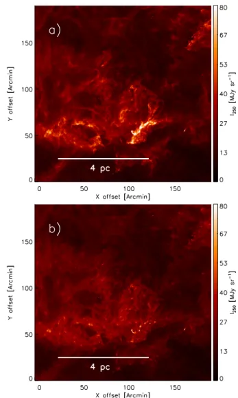
In this section, we analyze the Herschel/SPIRE image of the Polaris Flare cloud at 250 µm (Miville-Deschênes et al. 2010; Ward-Thompson et al. 2010; see also Schneider et al. 2013), which covers an area of 3.0◦× 3.3◦ and is shown in Fig.3a) at
the native (diffraction-limited) beam resolution of 18.002. For our
analysis, a pixel size of 600was adopted3.
The Polaris Flare image displays a spectacular distribution of low column density filaments. All of these filaments are ther-mally subcritical. The mean peak surface brightness contrast of these filaments over the local background is around hδci ∼ 0.9,
but the filaments occupy only a small fraction ∼2% of the total surface area, leading to δ2cAfil∼ 0.016.
To first order, the transverse structure of the Polaris fila-ments is well described by Gaussian profiles with a FWHM of ∼0.1 pc (assuming a distance ∼140 pc for the Polaris cloud) (Arzoumanian et al. 2011, 2019). Miville-Deschênes et al. (2010) carried out a power spectrum analysis for the Polaris image over spatial scales ranging from 0.01 pc to 10 pc. The power spectrum revealed a continuous power-law, P(k) ∝ kγ, with an exponent of γ = −2.65 down to the scale of the
3 A zero-level offset of 16.8 MJy/sr was also added to the image based
on a comparison with Planck and IRAS data.
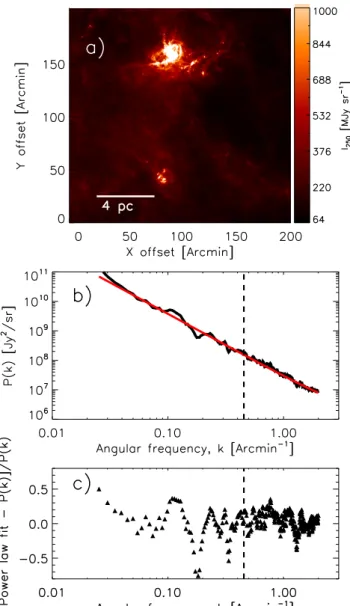
Fig. 3.Panel a: Herschel/SPIRE 250 µm emission image of a part of the
Polaris cloud. The HPBW angular resolution is 18.00
2. Panel b: noise-subtracted and beam-corrected power spectrum of the image shown in panel a over the range of angular frequencies 0.025 arcmin−1 <
k < 2 arcmin−1. The red curve shows the best fit power-law model
over this frequency range, which takes the form Psky(k)= AISMkγ+ P0
with γ= −2.63 ± 0.1. Panel c: residuals between the best-fit power-law model and the power spectrum data points (triangle symbols). The χ2
Variance(see Eq. (10)) of the residuals is ∼0.03. The vertical dashed line
marks the angular frequency kfil∼ (0.6/θfil) corresponding to a
charac-teristic filament width of ∼0.1 pc.
beam, suggesting a scale-free image. Following the same scheme as Miville-Deschênes et al. (2010), we derived the power spectrum of a sub-field4 of Polaris shown in Fig. 3.
Prior to computing of power spectrum, we apodized the edges of the image by a sine function to ensure smooth periodic boundary condition. After subtracting the noise power spectrum level estimated from the mean power at angular frequencies k > 3.5 arcmin−1, we corrected for convolution effects by 4 In order to capture the maximum rectangular area within the Polaris
image for easier computation of the power spectrum, we rotated the original map in equatorial coordinate by 13.6◦
clockwise about its cen-ter and extracted the largest area excluding turn-around data points near the edges of the field.
dividing the observed power spectrum by the power spectrum of the Herschel telescope beam at 250 µm (Martin et al. 2010) obtained from scans of Neptune. In order to derive the power spectrum slope, we then fitted a power-law model of the form Psky(k)= AISMkγ+ P0to the corrected power spectrum over the
range of angular frequencies 0.025 arcmin−1 < k < 2 arcmin−1, as described in Miville-Deschênes et al. (2010). In Fig. 3b, we show the power spectrum of the Polaris image over the range of angular frequencies used in the power-law fit. The red curve represents the best-fit power law with γ= −2.63 ± 0.1, which is very close to the γ= −2.65 ± 0.1 value obtained by Miville-Deschênes et al. (2010). Visual inspection shows that there is no clear spectral signature of a characteristic scale embedded in the observed power spectrum. Figure 3c shows the residuals [PBest−fit(k) − PPolaris(k)]/PPolaris(k) as a function
of angular frequency. Any significant kink or distortion in the power spectrum due to the presence of a characteristic scale should in principle be captured as a significant deviation from zero in the plot of residuals. The plot of residuals for the Polaris Flare image (Fig. 3c) does not exhibit such a deviation.
In order to critically analyze this finding, we performed a suite of numerical experiments by injecting synthetic filaments separately into 1) the original Herschel/SPIRE 250 µm image of Polaris, and 2) the filament-subtracted image obtained after applying the getfilaments algorithm (Men’shchikov 2013) to the Herschel/SPIRE image to remove most of the real filamentary structures. We repeated the same power spectrum analysis as described above on both sets of modified Herschel images (see Sects.4.2and4.3below). For this analysis, we preferred to use SPIRE 250 µm data rather than 18.002 column density images produced from the combination of Herschel data at 160 µm to 500 µm (cf.Palmeirim et al. 2013) because the former are less affected by noise and better behaved from a power-spectrum point of view (cf.Miville-Deschênes et al. 2010).
4.1. Construction of an image with synthetic filaments To create a synthetic filament image, the first step was to gen-erate a map of randomly oriented 1D delta line functions as described in Sect. 2. Then, we convolved this initial synthetic map with a Gaussian kernel such that the projected spatial FWHM width of the kernel was 0.1 pc as described in Sect.2. When creating synthetic filaments we neglected the fluctua-tions observed along real Herschel filaments (Roy et al. 2015), because the contrast of these fluctuations above the average filament is 1, and also the area filling factor of these fluc-tuations is very small. To maximize the effect of a character-istic width in our simulations, we fixed the FWHM width of the Gaussian filaments to a strictly constant value. We con-trolled the contrast parameter C of each filament by measur-ing the local background emission in the close vicinity of the filament within the background image. The distribution of the contrast parameter was chosen to reflect the observed distri-bution in each region. In the simulation, we varied the angu-lar length of the filaments randomly between a minimum of 30 × 18.002= 54600and a maximum of 70 × 18.002= 127400, corre-sponding to 0.4 to 0.9 pc at d = 140 pc. Figure 4a shows one such realization including a population of synthetic filaments with a lognormal distribution of contrasts in the range 0.3 < δc<
2.0, co-added to the original map of Polaris. In this example, the population of synthetic filaments has an area filling factor Afil∼ 3.2%.
4.2. Effect of synthetic filaments on the power spectrum of the Polaris image
Next, we investigated the effect of synthetic filaments on the power spectrum of the Polaris original image on one hand, and the power spectrum of the filament-subtracted Polaris image on the other hand. First, we discuss the case of the Polaris original image.
Figure 4b shows the total power spectrum of the Polaris image in Fig.4a, which includes a population of synthetic fil-aments with a log-normal distribution of contrasts, δc. In Fig.4,
the range of contrast values in the synthetic distribution varied in the range 0.3 < δc < 2.0 with a peak at δpeak ∼ 0.9. The
weighted average of the contrast over the length of the simu-lated filaments is hδci ∼ 0.85. In Fig. 4a, the synthetic
fila-ments are clearly visible against their local background. The best power-law fit to the power spectrum (red curve) has a logarith-mic slope γ= −2.7 ± 0.1, slightly steeper than the slope of the Polaris original image. The vertical dashed line marks the angu-lar frequency, kfil= Γ ∼ (0.6/θfil) ∼ 0.24 arcmin−1,
correspond-ing to the characteristic angular width of the synthetic filaments, θfil = 14700 (i.e., 0.1 pc at d= 140 pc). Comparison of Figs.4b
and3b shows that the synthetic filaments contribute an insignif-icant amount of power around kfil = 0.24 arcmin−1, which can
hardly be detected without prior knowledge of the power spec-trum of the original ISM image. Figure4c plots the normalized residuals between the best power-law fit and the power spectrum data, [PBest−fit(k) − PPolaris(k)]/PPolaris(k), as a function of angular
frequency. These residuals (red filled circles) can be compared with the residuals obtained with the original image, represented by black triangles in both Figs.3c and4c. Again, no clear sig-nature of the presence of synthetic filaments can be detected despite the fact that they have a characteristic width.
Now let us investigate the power spectrum of each compo-nent more closely to understand the absence of any detectable signature in the total power spectrum. The blue curve and the green dashed curve in Fig.4b show the power spectrum of the synthetic filament image and that of the original image, respec-tively. Note that the power spectrum of the filament image, Pfil(k), is lower than the power spectrum PPolaris(k) at k = kfil
by a factor of ∼5. This is because the population of synthetic filaments only have moderate area filling factor (Afil ∼ 3.2%)
and contrast (hδci ∼ 0.85). In this experiment, the product of
the area filling factor with the square of the column density contrast (Afilδ2c ∼ 0.02) was in agreement with the real
fila-ments observed in Polaris (which have Afilhδci2 ∼ 0.01 – cf.
Arzoumanian et al. 2019). The additional power introduced by the synthetic filaments is not localized in the vicinity of kfilbut
rather spread out at angular frequencies k. kfil, following a
shal-low power-law, whereas the power at high angular frequencies at k> kfildrops sharply. Given the choice of δcand Afilmade here,
the relative contribution of filaments to the total power spectrum, Pfil(k)/PPolaris(k) is highest in the vicinity of kfil, but too small to
create any detectable feature in the power spectrum.
When the contrast and/or filling factor of the synthetic filaments is gradually increased, the spectral imprint in the resulting power spectrum becomes more and more pronounced. FigureB.2a shows a simulated image including a population of synthetic 0.1 pc filaments with contrast δc ∼ 1.1 and area
fill-ing factor Afil ∼ 7.2%. This is quite an extreme scenario for
a non-star-forming molecular cloud with low column density such as Polaris. Figure B.2b shows the corresponding power spectra, which should be compared to those in Fig. 4b. It can be seen that the amplitude of the synthetic power spectrum in
Fig. 4.Same as Fig.3but for a 250 µm image with an additional popu-lation of synthetic filaments. The popupopu-lation of synthetic filaments has a lognormal distribution of contrasts in the range 0.3 < δc < 2.0 with
a broad peak around δpeak ∼ 0.9. The overall area filling factor of the
synthetic filaments is Afil ∼ 3% and the δ2cAfilparameter (see Sect.3)
is 0.023. Panel b: solid black curve shows the total power spectrum of the original Polaris image plus synthetic filaments. The best-fit power-law (red curve) has γ= −2.7 ± 0.1, slightly steeper than the slope of the original power spectrum of the Polaris image shown by the dashed green curve. The blue curve is the power spectrum of the image contain-ing only synthetic filaments. Panel c: black triangles are the same as in Fig.3c and the red dots show the residuals between the best-fit power-law model and the power spectrum of the image including synthetic fil-aments. The χ2
varianceof the residuals between kmin< k < 1.5 kfilis 0.037.
The vertical dashed line marks the angular frequency kfil ∼ (0.6/θfil)
corresponding to the characteristic ∼0.1 pc width of the synthetic filaments.
AppendixB(with contrast hδci ∼ 1.1 and Afil∼ 7.2%) is higher
by a factor of 3 to 4 than the amplitude of the power spec-trum of Fig. 4b (with contrast hδci ∼ 0.85 and Afil ∼ 3.2%),
mostly due to the increase in the combination of contrast param-eter and area-filling factor hδci2Afilbetween the two simulations
[∼(1.1/0.85)2 × (7.2/3.2)(∼3.7)]. The red curve in Fig. B.2b shows the best power-law fit which has a logarithmic slope γ = −2.96 ± 0.1. At k . kfil, there is a significant
enhance-ment of power due to the fact the synthetic filaenhance-ment power spec-trum Pfil(k) is now comparable to the Polaris power spectrum
PPolaris(k) at k . kfil. Accordingly, in this case, the residuals
between the best power-law fit and the total power spectrum data depart significantly from zero at k . kfil(cf. Fig.B.2c). It is to
be borne in mind, however, that the population of synthetic fila-ments used in AppendixBhave much higher contrast and area filling factor than the actual filaments of the Polaris cloud (com-pare Figs.B.2a and3a).
4.3. Effect of synthetic filaments on the power spectrum of the filament-subtracted image
So far we have explored the response of the power spectrum to a synthetic population of filaments injected into the original Herschelimage, which itself includes emission from real fila-mentary structures. It is instructive to assess the extent to which the real filaments present in the image may reduce the rela-tive contribution of synthetic filaments. In order to evaluate this we adopted two approaches – first, we subtracted the emis-sion of at least the most prominent real filamentary structures from the Polaris 250 µm image using the getfilaments algorithm (Men’shchikov 2013, see Fig.B.1b for the resulting filament-subtracted image) and then repeated the same experiment as described in Sect.4.1. Second, we examined the effect of fila-ments embedded in a typical scale-free synthetic cirrus images (see AppendixC). In order to be consistent, we used the same population of synthetic filaments as in Sects.4.1and4.2.
Figure 5summarizes the effect of the synthetic 0.1 pc fila-ments on a background image which is essentially devoid of real filamentary structures. Although the logarithmic power-spectrum slope of the background image is shallower (γbkg = −2.5) than
that of the Polaris original image (γobs= −2.7), the overall
mor-phology remains the same. In particular, the power spectrum of the synthetic filament component is still significantly lower than the total power spectrum of the background image, even though the power arising from real filaments has been subtracted from that image. The χ2
varianceof the filament-subtracted background image
is 0.04, very close the χ2
variancevalue obtained for the Polaris
orig-inal image. Moreover, there is still no clear signature of the pres-ence of synthetic filaments in the residuals plot (Fig.5c). Similar conclusions were reached in AppendixCin the case of synthetic filaments added to a purely synthetic background image.
5. Exploring the parameter space with simulations in the Aquila cloud
The Aquila molecular cloud harbors a statistically significant number of filaments with a wide range of filament column den-sity contrasts (Könyves et al. 2015; Arzoumanian et al. 2019), allowing us to derive a realistic distribution of contrasts which can then be used for constructing more realistic populations of synthetic filaments.
5.1. Observed filament properties in Aquila
In contrast to the Polaris cloud, the Aquila molecular cloud is an active star forming complex at a distance5 of 260 pc, including
several supercritical filaments (André et al. 2010;Könyves et al. 2015). Figure6a shows the Herschel/SPIRE 250 µm image of the
5 The distance of the Aquila cloud is uncertain, with values ranging
from 260 pc to 414 pc in the literature. Assuming the upper distance value would push kfiltoward higher angular frequencies in Fig.6b and
c, making the detection of the 0.1 pc scale even more difficult in the power spectrum.
Fig. 5. Same as Fig. 4 for synthetic filaments added to a filament-subtracted image of Polaris obtained with getfilaments (Men’shchikov 2013). The population of synthetic filaments is the same as that in Fig.4. Panel b: green dashed line shows the best power-law fit to the power spectrum of the filament-subtracted background image of Polaris (with no synthetic filaments), which has a slope of γ= −2.4 ± 0.1. The solid black curve shows the total power spectrum of the filament-subtracted image plus synthetic filaments. The best-fit power-law (red curve) has a slope of γ= −2.5 ± 0.1, slightly steeper than the slope of the power spec-trum of the filament-subtracted background image (dashed green curve). The blue curve is the power spectrum of the image containing only syn-thetic filaments. Panel c: black triangles are the same as in Fig.3c and the red dots show the residuals between the best-fit power-law model and the power spectrum of the image including synthetic filaments. The χ2
varianceof the residuals between kmin< k < 1.5 kfilis 0.034. The vertical
dashed line marks the angular frequency kfil ∼ (0.6/θfil) corresponding
to the characteristic ∼0.1 pc width of the synthetic filaments.
Aquila cloud, which covers a projected sky area of 3.4◦× 3.2◦. The corresponding power spectrum is shown in Fig.6b.
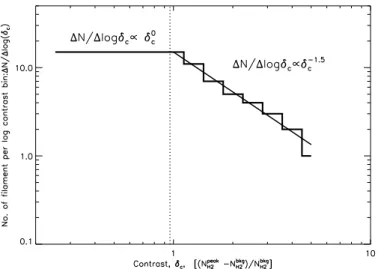
As part of a systematic analysis of filament properties in nearby clouds based on HGBS data,Arzoumanian et al.(2019) took a census of filamentary structures in Aquila. They obtained a distribution of filament column density contrasts which can be conveniently approximated by the two-segment power law shown in Fig. 7: dN/dlog(δc) ∼ const for 0.3 ≤ δc ≤ 1, and
dN/dlog(δc) ∼ δ−1.5c for 1 ≤ δc ≤ 4. This observed distribution
of filaments contrasts has a peak around δpeakc ∼ 1 and spans
Fig. 6. Panel a: Herschel/SPIRE 250 µm image of the Aquila cloud
at the native resolution of 18.00
2. Panel b: noise-subtracted and beam-corrected power spectrum of the image shown in panel a over the range of angular frequencies 0.025 arcmin−1< k < 2 arcmin−1(black curve).
The red curve shows the best fit power-law model over this frequency range, which has a logarithmic slope γ = −2.26 ± 0.1. The verti-cal dashed line marks the angular frequency kfil ∼ (0.6/θfil−width) ∼
0.45 arcmin−1 corresponding to a filament width of θ
fil−width=7900
(FWHM), i.e., 0.1 pc at a distance of 260 pc. Panel c: residuals between the best power-law fit and the power spectrum data points (triangle symbols). The χ2
Varianceof the residuals between kmin < k < 1.5 kfil is
∼0.045.
a broad range from low δc ∼ 0.3 values to fairly high δc ∼ 4
values. The weighted average column density contrast of the filaments observed in Aquila is hδci ∼ 1, and their area
fill-ing factor is Afil ∼ 3%. While the census of filaments obtained
by Arzoumanian et al. (2019) may be affected by incomplete-ness issues for low-contrast6 (δc 1) filaments, it should be
essentially complete for high-contrast (δc & 1) supercritical
filaments.
6 Given the fact that the amplitude of a power spectrum ∝δ2 c,
unde-tected filaments (with low contrasts) below the completeness level will not have any significant effect on the net amplitude of synthetic fila-ments power spectrum.
Fig. 7.Two-segment power-law approximation (black solid lines) to the distribution of filament column density contrasts observed in the Aquila molecular cloud (Arzoumanian et al. 2019): dN/dlog(δc) ∼ const for
0.3 ≤ δc ≤ 1, and dN/dlog(δc) ∼ δ−1.5c for 1 ≤ δc ≤ 4. The vertical
dotted line marks the average filament contrast hδci ∼ 1. The
overplot-ted histogram shows the distribution of column density contrasts for the population of 100 synthetic filaments used in the simulation of Sect.4.
5.2. Effect of a synthetic population of filaments on the power spectrum
Using a methodology similar to that employed in Sect. 4 for Polaris, we added a population of synthetic filaments with fixed 0.1 pc width to a filament-subtracted Herschel image of the Aquila region at 250 µm. The distribution of column density con-trasts7for the synthetic filaments was constructed to be consis-tent with observations and is represented by the histogram in Fig.7. The weighted mean contrast of the whole population of synthetic filaments was hδci ∼ 0.96. Like in the Polaris case,
the background image was obtained from the Herschel/SPIRE 250 µm of the Aquila cloud image after removing observed fil-aments using the getfilfil-aments algorithm (Men’shchikov 2013). The resulting synthetic image is shown in Fig. 8a. Figure 8b shows the power spectrum of each component in the synthetic image: the blue curve corresponds to the contribution of the syn-thetic filament distribution, while the black curve is the total power spectrum of the Aquila background plus filament image.
It can be seen in Fig.8b that the amplitude of the power spectrum arising from the population of synthetic filaments (blue curve) is lower than the amplitude of the power spectrum of the Aquila original image (green dashed curve) by a factor of ∼5 at k ∼ kfil∼ (0.6/θfil) ∼ 0.45 arcmin−1, corresponding to the
char-acteristic angular width of the synthetic filaments, θfil= 7900(i.e.,
0.1 pc at d= 260 pc). Clearly, the power contribution of the syn-thetic filaments is not strong enough to be detected in the power spectrum. The residuals of the best power-law fit with respect to the power spectrum of the Aquila original image are shown as black triangles in Fig.8c as a function of angular frequency. The red solid circles in Fig. 8c represent similar residuals for the Aquila background plus synthetic filament image. Based on this simulation, we conclude that the injection of a population
7 The column density contrasts of cold molecular filaments are
some-what higher than their surface brightness contrasts at 250 µm. To be on the conservative side, we used the observed distribution of column den-sity contrasts for constructing synthetic filaments in the 250 µm images. The actual surface brightness contrasts are actually lower than what we assumed here.
Fig. 8.Same as Fig.6but for a simulated image including a
popula-tion of synthetic filaments with a realistic distribupopula-tion of column density contrasts (see Fig.7) added to a filament-subtracted image of the Aquila cloud. Panel a: simulated image. The weighted average contrast hδci of
the distribution of synthetic filaments is 0.96 and the total area covering factor Afilis 5.5%, leading to δ2cAfil ∼ 0.051. Panel b: power spectrum
of the simulated image (black solid curve). The red curve corresponds to the best power-law fit with γ = −2.3 ± 0.1. For comparison, the best power-law fit to the power spectrum of the Aquila original image is over-plotted as a green dashed line. Panel c: residuals between the best power-law fit and the power spectrum of the simulated image (red solid circles). The χ2
Variance of the residuals is ∼0.054 For comparison,
the black filled triangles show similar residuals for the Aquila original image (cf. Fig.6c).
of synthetic filaments with a distribution of column density con-trasts similar to that observed in the real Aquila image does not have any significant effect on the shape of the power spectrum.
In AppendixB, we also explore a more extreme case where the distribution of column density contrasts for the injected syn-thetic filaments is similar in shape to the distribution shown in Fig.7, but with higher mean contrast hδpeakc i = 2.7 and
maxi-mum contrast δmax
c = 15. In this extreme case, the population
of synthetic filaments is strong enough to produce a detectable signature in the resulting power spectrum.
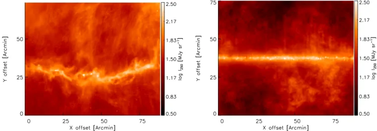
Fig. 9.Left panel: Herschel/SPIRE 250 µm image of the B211/B213 region in Taurus at the native beam resolution of 18.200
, but rotated in equatorial coordinates in clockwise direction by 37.4◦
. (seePalmeirim et al. 2013). Right panel: fully synthetic image mimicking the main features of the real image shown in the left panel, and resulting from the co-addition of a synthetic filament image and a synthetic background image. The synthetic filament image was based on the Plummer-like model of the B211 filament reported byPalmeirim et al.(2013): flat inner radius Rflat= 0.035 pc, contrast δc∼ 6, and power-law index p= 2 at large radii. The background image was modeled as non-Gaussian cirrus fluctuations
with a logarithmic power spectrum slope of −3 (see text for details), plus low-contrast filamentary structures resembling striations. The synthetic striations were placed such that their long axis is perpendicular to the main filament at a regular separation of 0.1 pc.
6. Power spectrum of synthetic data with a single, prominent filament
We also examined the power spectrum of an image with a single dominant filament such as the Herschel/SPIRE 250 µm image of the B211/B213 region in the Taurus cloud at d ∼ 140 pc (Fig.9a)8. For the present purpose, we only used a 1.2◦× 1.0◦
portion of the original SPIRE image of B211/B213, where a sin-gle filament dominates over a length scale of >1.5◦(or >4 pc).
Palmeirim et al.(2013) studied the column density structure of the B211/B213 filament in detail and found that it is accurately described by a Plummer-like cylindrical density distribution with flat inner radius Rflat ∼ 0.035 pc and power-law index p= 2±0.2
at larger radii up to an outer radius Rout ∼ 0.4 pc. Moreover,
Palmeirim et al.(2013) suggested that the Taurus main filament accretes mass from the ambient cloud through a network of lower-density striations, observed roughly perpendicular to the main filament. Based on these findings, we constructed a syn-thetic image of a Plummer-like filament of length ∼4 pc, with the same Plummer parameters as quoted above, and positioned horizontally in a ∼1.5◦× 1.5◦ two-dimensional box. The
con-trast of the synthetic filament was chosen to be δc∼ 6, a value
close to the observed contrast of the B211/B213 filament in the SPIRE 250 µm image (seePalmeirim et al. 2013). To mimic the observations, we added a population of synthetic cores with Bonnor-Ebert-like radial profiles randomly distributed along the filament. The flat inner radius Rflatof the cores was fixed to a
con-stant value of 0.02 pc. In order to create a synthetic background image similar to the real data, we carefully studied the statisti-cal properties of the Herschel 250 µm image in the vicinity of the Taurus main filament. We selected a rectangular field to the north of the B211/B213 main filament such that the nearest edge of the field was at least 0.2 pc away from the filament crest. We then evaluated the power spectrum of this field and found a log-arithmic slope γ ∼ −3.0 ± 0.2. A purely synthetic background image was next generated using a non-Gaussian fractional
Brow-8 In order to capture the largest possible rectangular area, we rotated
the SPIRE map by 37.4◦
in the clockwise direction with respect to an equatorial frame.
nian motion (fBm) technique (Miville-Deschênes et al. 2003) with positive values and statistics such that the power spec-trum of the background field had a logarithmic slope simi-lar to that of the Taurus background field (γback = −3.0). To
make the synthetic background image more similar to the Taurus observations, we also inserted a distribution of lognormally dis-tributed low-contrast (0.1 < δc< 0.5) filamentary structures with
Gaussian profiles perpendicular to the main filament as a proxy for the observed striations. We placed perpendicular striations at a regular separation of ∼0.1 pc to match the observations of Tritsis & Tassis(2018). The width of these synthetic striations was fixed to 0.08 pc.
The final image, obtained after co-adding all three synthetic image components (background, striations, and main filament with embedded cores), is shown in Fig.9b. For reference and comparison with the synthetic data discussed in Sects.4and5, this image has δ2cAfil ∼ 0.125. Figure10compares the power
spectrum of the synthetic image (red curve) with that of the Herschel/SPIRE 250 µm image (black solid curve). The vertical dashed line in Fig.10marks the angular frequency kfil
correspond-ing to a linear scale of ∼0.1 pc, i.e., roughly the inner width of both the synthetic filament and the B211/B213 filament. Clearly, like for the other two regions considered in this paper, the power spec-trum of the Taurus B211/B213 data does not reveal any “kink” or “break” at frequencies close to kfil. Furthermore, this is also the
case for the synthetic data of Fig.9b, despite the presence of a prominent cylindrical filament with ∼0.1 pc inner diameter. This further illustrates how the characteristic scale of embedded struc-tures may be hidden and undetectable in a global power spectrum.
7. Combined effect of filament contrast and area filling factor
In order to further explore the dependence of the total power spec-trum on filament contrast and area filling factor, we performed two separate grids of 20 × 20 Monte-Carlo simulations based on two different sets of synthetic filament populations, one with Gaussian radial profiles and the other with Plummer-like profiles with p = 2 (see AppendixA). The simulated images spanned a
Fig. 10. Comparison of the power spectrum of the Herschel/SPIRE
250 µm image of Fig.9a (black solid curve) with that of the synthetic image of Fig.9b (red curve). Note the absence of any significant feature around k ∼ kfil(vertical dashed line) in both power spectra.
broad range of average filament contrasts hδci and filling factors
Afil. In practice, we injected a fixed number of synthetic filaments
of 0.1 pc width in the Herschel/SPIRE 250 µm image of Polaris and controlled the area filling factor by varying the length of the filaments. For each realization, we then calculated the χ2varianceof the residuals between the best power-law fit and the net output power spectrum, as described in Sect.3.
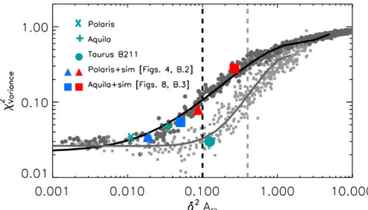
Figure11summarizes the dependence of χ2varianceon hδci2and
Afilfor Gaussian synthetic filaments. The map of the χ2varianceas a
function of hδci2and Afilis qualitatively similar for Plummer-like
synthetic filaments. Figure12shows that there is a tight corre-lation between χ2
varianceand hδci 2× A
filfor both Gaussian (black
solid circles) and Plummer-like filaments (gray solid squares), as expected from Eq. (12). In both cases, χ2
variance appears to be
a non-linear function of δ2
cAfil, with a flat portion at low δ2cAfil
values (i.e., δ2cAfil . 0.02 for Gaussian filaments, δ2cAfil .
0.07 for Plummer-like filaments), a rising portion at higher δ2 cAfil
values, with an inflection point close to δ2cAfil ∼ 0.1 in the
Gaussian case and δ2
cAfil∼ 0.4 in the Plummer case (see Fig.12).
It can also be seen that, for the same value of δ2cAfil, the χ2varianceis
lower for Plummer synthetic filaments than for Gaussian synthetic filaments9.
Qualitatively, this behavior may be understood as follows. At low δ2
cAfil. 0.02 values (or δ2cAfil. 0.07 for Plummer-like
filaments), the contribution of synthetic filaments to the total power spectrum is negligible, and χ2
Variance is dominated solely
by the residuals of the original background image. There-fore, χ2
variance retains the value χ 2
variance,bkg it has for the
orig-inal image and remains constant despite the addition of syn-thetic filaments. As δ2
cAfil increases, the χ2variance for both
Gaussian and Plummer filaments also increases, reaching a value of about 3 × χ2
variance,bkg∼ 0.1 at δ 2
cAfil∼ 0.1 (Gaussian case) or
0.4 (Plummer case). We take these values of δ2cAfilas fiducial
limits for the detection of a characteristic filament width in the image power spectrum for Gaussian- and Plummer-shaped fila-ments, respectively. These fiducial detection limits are marked by black and gray vertical dashed lines in Fig.12.
To put the simulation results shown in Figs.11and12in con-text, we recall that the Polaris simulation of Fig.5a in Sect. 3 had
9 A Plummer-like filament with p. 2.6 contributes less power to the
power spectrum at low angular frequency than a Gaussian filament with similar inner width and contrast (see Fig. 2b). Therefore, at k < kfil,
Plummer-like filaments with p . 2.6 lead to a lower overall χ2 Variance
compared to Gaussian filaments.
Fig. 11. Map of the χ2− variance of the residuals between the best
power-law fit and the output power spectrum as a function of column density contrast (δc) and area filling factor (Afil) in a grid of simulations
based on a set of 20 × 20 populations of Gaussian synthetic filaments, all 0.1 pc in width (see text of Sect.7for details). The white solid curve marks the fiducial limit δ2
cAfil= 0.1 above which the effect of the
char-acteristic filament width can be detected in the power spectrum (see Fig.12below). The white plus and cross symbols mark the positions of the observed populations of filaments in the Aquila and Polaris clouds, respectively (cf.Arzoumanian et al. 2019).
δ2
cAfil∼ 0.018 and χ2varianceof 0.034 (see Fig.4c), which is nearly
the same as the observed χ2
variance,bkg∼ 0.04 (see Fig.3). This
par-ticular simulation is marked by a blue triangle in the χ2 variance–
δ2
cAfilplot of Fig.12. The more extreme Polaris simulation
pre-sented in Fig.B.2a, for which there is a marginal detection of a characteristic scale in the residuals plot (see Fig. B.2c), has δ2
cAfil ∼ 0.087 and χ2variance ∼ 0.08 (see red triangle in Fig.12).
Likewise, the blue and red square symbols in the χ2variance– δ2cAfil
plot of Fig.12mark the positions of the two sets of Aquila sim-ulations presented in Figs.8andB.3, respectively.
The red square in Fig.12has δ2
cAfil ∼ 0.27 (and χvariance ∼
0.28), significantly above the fiducial detection limit of 0.1, indi-cating that the signature of a characteristic filament width should be detectable in the power spectrum. This is indeed confirmed by visual inspection of Fig. B.3b and c. Most importantly, for both Polaris and Aquila, the real Herschel data lie in a por-tion of the χ2variance– δ2cAfil diagram where the filament
contri-bution has a negligible impact on the power spectrum (see cross and plus symbols in Figs. 11and12). Also shown as a green filled circle in Fig.12is the locus of the Herschel data for the prominent filament system B211/B213 in Taurus (see Sect.6), which has a very well characterized Plummer-like density pro-file with a power-law wing index p = 2 ± 0.2 (Palmeirim et al. 2013). It can be seen that the position of the Taurus B211/B213 data in Fig.12is in excellent agreement with our set of simu-lations for Plummer-shaped filaments with p= 2. Although the δ2
cAfil ∼ 0.125 value of the Taurus B211/B213 data is greater
than the fiducial threshold for Gaussian filaments, it remains much lower than the fiducial detection limit for Plummer (p= 2) filaments.
We conclude that the essentially scale-free power spectrum of the Herschel images observed toward molecular clouds such as Polaris, Aquila, or Taurus does not invalidate the existence of a characteristic filament width.
Fig. 12.χ2
Varianceof the residuals between the best power-law fit and the
output power spectrum as a function of δ2
cAfil. The black solid circles
rep-resent the same set of simulations with Gaussian filaments as in Fig.11. The light gray squares represent our set of simulations with Plummer-like (p= 2) filament profiles. The corresponding black and gray curves are polynomial fits to guide the eye. The black and gray vertical dashed lines mark the fiducial limits of δ2
cAfil∼ 0.1 and δ2cAfil∼ 0.4 above which
Gaussian-shaped and Plummer-shaped filaments become detectable in the residual power spectrum plot, respectively. The green cross, plus, and solid circle symbols mark the positions of the Polaris, Aquila, and Tau-rus clouds, respectively, based on the comprehensive study of filament properties byArzoumanian et al.(2019).
8. Summary and conclusions
We used numerical experiments to investigate the conditions under which the presence of a characteristic filament width can manifest itself in the power spectrum of cloud images. Our main findings and conclusions may be summarized as follows:
1. The detectability of a characteristic filament scale in the power spectrum of an ISM dust continuum image primarily depends on the parameter δ2cAfil, where δc is the weighted
average column density contrast of the filamentary struc-tures and Afiltheir area filling factor in the image. A value
δ2
cAfil ' 0.1 is required for the presence of a characteristic
filament width to produce a significant signature in the power spectrum.
2. The Herschel Gould Belt survey images of nearby clouds typically have δ2cAfil 0.1 and therefore lie in a region of
the parameter space where filaments have a negligible impact on the power spectrum. Therefore, despite recent claims, the scale-free nature of the observed power spectra remains con-sistent with the presence of a characteristic filament width ∼0.1 pc.
3. When the average filament contrast is low and/or when the filaments occupy a small area filling factor, the power spec-trum is dominated by the fluctuations of the diffuse, non-filamentary component of the ISM.
4. Although a few filaments in the Polaris cloud have column density contrasts up to δc ∼ 0.9, their area filling factor is
extremely low Afil ∼ 2%, resulting in a combined
parame-ter δ2
cAfil∼ 0.01 for Polaris. The overall power spectrum of
the Herschel images of Polaris is scale-free because the fil-aments are not contributing enough power to produce a sig-nificant signature at the spatial frequency corresponding to the characteristic filament width of ∼0.1 pc.
5. Despite the presence of several supercritical filaments of ∼0.1 pc inner width in the Aquila cloud, the power spectrum of the Aquila Herschel images is also essentially scale free. Due to the larger distance of the Aquila cloud compared to Polaris, ∼0.1 pc filaments in Aquila subtend a smaller
angu-lar width scale on the sky, and therefore have a relatively low area filling factor. Overall, our simulations suggest that the observed population of Aquila filaments contributes only ∼1/5 of the total amplitude of the power spectrum of the Herschel250 µm image.
6. Supercritical filaments with Plummer-like profiles and high column density contrasts lead to relatively small departures from a power-law power spectrum because the high contrast of the flat inner plateau in the density profile is compensated by broad power-law wings at large radii. The B211/B213 fil-ament system in Taurus, for example, despite having a very high central column density contrast, remains largely unde-tected in the image power spectrum because of its Plummer-like density profile with p ≈ 2.
7. We conclude that the scale-free appearance of the power spectra of cloud images does not invalidate the finding, based on detailed Herschel studies of the column density profiles, that nearby molecular filaments have a common inner width ∼0.1 pc (Arzoumanian et al. 2011,2019).
Acknowledgements. This work has received support from the European Research Council under the European Union’s Seventh Framework Pro-gramme (ERC Advanced Grant Agreement no. 291294 – “ORISTARS”). We also acknowledge financial support from the French national programs of CNRS/INSU on stellar and ISM physics (PNPS and PCMI). A.R, and N.S., acknowledge support by the French ANR and the German DFG through the project “GENESIS” (ANR-16-CE92-0035-01/DFG1591/2-1). P.P. acknowl-edges support from the Fundação para a Ciência e a Tecnologia of Portugal (FCT) through national funds (UID/FIS/04434/2013), from FEDER through COMPETE2020 (POCI-01-0145-FEDER-007672), and from the fellowship SFRH/BPD/110176/2015 funded by FCT (Portugal) and POPH/FSE (EC). We are grateful to our colleague Alexander Men’shchikov for assistance with the getfilaments algorithm. This research has made use of data from the Herschel Gould Belt survey (HGBS) project (http://gouldbelt-herschel.cea.fr). The HGBS is a Herschel Key Programme jointly carried out by SPIRE Specialist Astronomy Group 3 (SAG 3), scientists of several institutes in the PACS Con-sortium (CEA Saclay, INAF-IFSI Rome and INAF-Arcetri, KU Leuven, MPIA Heidelberg), and scientists of the Herschel Science Center (HSC).
References
André, P., Men’shchikov, A., Bontemps, S., et al. 2010,A&A, 518, L102 André, P., Di Francesco, J., Ward-Thompson, D., et al. 2014,Protostars and
Planets VI, 27
Arzoumanian, D., André, P., Didelon, P., et al. 2011,A&A, 529, L6 Arzoumanian, D., André, P., Könyves, V., et al. 2019,A&A, 621, A42 Auddy, S., Basu, S., & Kudoh, T. 2016,ApJ, 831, 46
Falgarone, E., Panis, J.-F., Heithausen, A., et al. 1998,A&A, 331, 669 Federrath, C. 2016,MNRAS, 457, 375
Fischera, J., & Martin, P. G. 2012,A&A, 542, A77 Gao, Y., & Solomon, P. M. 2004,ApJ, 606, 271
Heiderman, A., Evans, II., N. J., Allen, L. E., Huard, T., & Heyer, M. 2010,ApJ, 723, 1019
Hennebelle, P., & André, P. 2013,A&A, 560, A68 Inutsuka, S., & Miyama, S. M. 1997,ApJ, 480, 681 Koch, E. W., & Rosolowsky, E. W. 2015,MNRAS, 452, 3435 Könyves, V., André, P., Men’shchikov, A., et al. 2015,A&A, 584, A91 Lada, C. J., Lombardi, M., & Alves, J. F. 2010,ApJ, 724, 687 Marsh, K. A., Kirk, J. M., André, P., et al. 2016,MNRAS, 459, 342
Martin, P. G., Miville-Deschênes, M.-A., Roy, A., et al. 2010,A&A, 518, L105 Men’shchikov, A. 2013,A&A, 560, A63
Miville-Deschênes, M.-A., Levrier, F., & Falgarone, E. 2003,ApJ, 593, 831 Miville-Deschênes, M.-A., Martin, P. G., Abergel, A., et al. 2010,A&A, 518,
L104
Palmeirim, P., André, P., Kirk, J., et al. 2013,A&A, 550, A38
Panopoulou, G. V., Psaradaki, I., Skalidis, R., Tassis, K., & Andrews, J. J. 2017, MNRAS, 466, 2529
Roy, A., André, P., Arzoumanian, D., et al. 2015,A&A, 584, A111 Schneider, N., André, P., Könyves, V., et al. 2013,ApJ, 766, L17 Shimajiri, Y., André, P., Braine, J., et al. 2017,A&A, 604, A74 Tritsis, A., & Tassis, K. 2018,Science, 360, 635
Appendix A: Construction of synthetic filaments with Plummer-like density profiles
Fig. A.1.Image of a synthetic filament with a Plummer-like transverse
density profile with a flat inner radius, Rflat = 0.03 pc, and a
power-law wing with index p = 2, projected at a distance of 140 pc. In this example, the level of filament contrast was adjusted to δc∼ 10.
We adopted a slightly different technique to produce filaments with Plummer profiles compared to the convolution technique used to generate filaments with Gaussian profiles (see Sect.2). A Plummer-like transverse profile was first constructed using the expression KPlummer(r)= C h 1+ (r/Rflat)2 i(p−1)/2, (A.1) where Rflat is the flat inner width and p is the logarithmic slope
of the power-law wing at large radii (r >> Rflat). In order to
sup-press the strong edge effect at the two ends of the model filament, we tapered both edges with a Gaussian function. Figure A.1 shows an example of synthetic filament with a Plummer pro-file p= 2 and Rflat= 0.1 pc, similar to the Taurus B211 filament
(Palmeirim et al. 2013). The power spectra of synthetic filaments with Plummer-like density profiles are discussed in Sect.2.
Appendix B: Effect of extreme filament contrasts and area filling factors on the power spectrum
FiguresB.2andB.3illustrate the consequences of adding pop-ulations of synthetic filaments with very high column density contrasts on the total power spectra of Polaris and Aquila, respectively. Figure B.2a displays the Herschel 250 µm image of the Polaris cloud populated with a set of high-contrast fila-ments with δc ∼ 1.1. The number of synthetic filaments was
fixed to 100 and the distribution of synthetic filament lengths was adjusted so that the overall area filling factor was around Afil∼ 7%. In this case, the synthetic filaments contribute a level
of power (blue curve) almost equivalent to the power spectrum of the Polaris original image (cf. dashed green curve). This leads to an enhancement of power in the total power spectrum, which can be clearly seen in the residuals plot (red filled circles in Fig.B.2c). The χ2− variance of the residuals of the power-law
Fig. B.1. Comparison of the Herschel/SPIRE 250 µm image of
Polaris at the native beam resolution of 18.200
(panel a –see
Miville-Deschênes et al. 2010) with the filament-subtracted image of
the same field, panel b obtained with the getfilaments algorithm
(Men’shchikov 2013) and used as a “filament-free” background image
in the numerical experiments shown in Figs.5andB.2.
fit in the angular frequency range of kmin < k < 1.5 kfilis about
seven times larger than the χ2− variance metric for the Polaris original image.
In the Aquila case, we created a population of 100 syn-thetic filaments rescaling the observed distribution of column density contrasts as shown in Fig.B.4. The maximum contrast sampled in the distribution was increased to δmax
c = 15
(com-pared to ∼3 in the original contrast distribution), and the peak of the distribution was shifted to δpeakc ∼ 2 compared to 1 in
the original distribution. The average contrast level of the syn-thetic filaments was about 2.2 and their area filling factor was as high as 5.5%. The resulting image obtained after adding this population of synthetic filaments to the Aquila original image is shown in Fig.B.3a. The power contribution due to the synthetic filaments, shown by the blue curve in Fig.B.3b, is significantly higher than the power spectrum amplitude of the Aquila orig-inal image (dashed green curve). Accordingly, the total power spectrum, [Pfil(k)+ PAquila(k), solid black curve in Fig. B.3b]
is amplified at angular frequencies k . kfil. A strong
devia-tion in the residuals plot (red symbols in Fig.B.3c) can also be seen.
Fig. B.2.Same as Fig.5but for a population of synthetic filaments with higher column density contrasts δc ∼ 1.1, resulting in δ2cAfil ∼ 0.087.
(The area filling factor is similar to that in Fig.4, Afil∼ 7.2%.) Panel b:
note how the amplitude of the power spectrum due to the synthetic fil-aments (blue curve) is comparable to that of the power spectrum of the Polaris original image (see green dashed line and Fig.3). The loga-rithmic slope of the total power spectrum P(k)fil+ P(k)Polarisis −2.96.
Panel c: residuals between the best power-law fit and P(k)Polaris+fil(red
solid circles) shows a peak near kfil ∼ 0.24 arcmin−1. In this
simula-tion, the χ2
varianceis 0.08, close to the fiducial detection limit δ 2 cAfil ∼ 1
introduced in Sect.7(see Fig.12).
Fig. B.3.Same as Fig.8but for a population of synthetic filaments
with a more extreme (and unrealistic) distribution of column density contrasts corresponding to hδci ∼ 2.2 (see Fig.B.4) and an area filling
factor Afil ∼ 5.5%, resulting in a combined parameter δ2cAfil ∼ 0.27.
Panel b: note how the power spectrum arising from the synthetic fil-ament population (blue curve) dominates over the power spectrum of the Aquila original image (see green dashed curve and Fig.6). The log-arithmic slope of the best power-law fit to the total power spectrum P(k)fil + P(k)Aquila is −2.6 (red line). Panel c: residuals between the
best power-law fit and P(k)Aquila+fil(red solid circles) shows a peak near
kfil,Aquila= 0.45 arcmin−1. For this simulation, the χ2Varianceof the residuals
Fig. B.4.Two-segment power-law distribution of synthetic filaments contrasts adopted in the Aquila simulations of AppendixB. The dis-tribution ranges from 0.3 to 15 and leads to a weighted average contrast of ∼2.2, significantly higher than in Fig.7.
Appendix C: Effect of filaments embedded in a scale-free synthetic background
We also generated a purely synthetic background image using the non-Gaussian fractional Brownian motion (fBm) technique of Miville-Deschênes et al. (2003), in such a way that the resulting power spectrum had a logarithmic slope γ = −2.7, mean brightness of the fluctuation ∼17 MJy/sr, and a standard deviation of 10 MJy/sr, similar to the statistics observed with Herschel in the Polaris field. On top of this scale-free image, a population of synthetic filaments with a lognormal distribu-tion of (δc) contrasts (similar to that observed in Polaris) was
added. The filaments had a Gaussian profile with an inner width of 0.1 pc projected at a distance of 140 pc, similar to the distance of the Polaris molecular cloud. They occupied an area-filling fac-tor Afil∼ 3% and had an average contrast δc∼ 0.8. The
result-ing synthetic image after co-addresult-ing the fBm background image and the synthetic filaments is shown in Fig.C.1a. Inspection of the various components of the image power spectrum (shown in Fig.C.1b) shows that the contribution of the synthetic filaments to the global power spectrum is negligible and undetectable in this case as well.
Fig. C.1. Purely synthetic image, made up of a scale-free
back-ground image constructed using the fBm algorithm (panel a; cf.
Miville-Deschênes et al. 2003). The embedded synthetic filaments have
a lognormal column density contrast distribution in a range between 0.3 < δc < 2 and peak of δpeak ∼ 0.9. The overall area-filling
factor of the filaments is Afil ∼ 3%. The filaments are of
Gaus-sian profiles with a FWHM ∼0.1 pc at a distance of 140 pc (see text). Panel b: solid black curve shows the power spectrum of the scale-free background image and the synthetic filaments. The logarithmic slope of the power-spectrum is γ ∼ −2.7 ± 0.1. The dashed curve shows the power spectrum of the background image (γ ∼ −2.8). The blue solid line shows the power spectrum of the synthetic filaments. Panel c: resid-uals between the best power-law fit and the power spectrum data points (triangle symbols) of synthetic cirrus map. The χ2
Varianceof the residuals