HAL Id: tel-01242486
https://hal.archives-ouvertes.fr/tel-01242486
Submitted on 14 Dec 2015
HAL is a multi-disciplinary open access
archive for the deposit and dissemination of
sci-entific research documents, whether they are
pub-lished or not. The documents may come from
teaching and research institutions in France or
L’archive ouverte pluridisciplinaire HAL, est
destinée au dépôt et à la diffusion de documents
scientifiques de niveau recherche, publiés ou non,
émanant des établissements d’enseignement et de
recherche français ou étrangers, des laboratoires
Networks
Matthieu de Mari
To cite this version:
Matthieu de Mari. Radio Resource Management for Green Wireless Networks. Other. SUPELEC,
2015. English. �tel-01242486�
SUPELEC
Ecole doctorale
“Sciences et Technologies de l’Information, des Télécommunications et des Systémes”
THESE DE DOCTORAT
DOMAINE: STIC Spécialité: Télécommunications
Soutenue le 1er Juillet 2015 par :
Matthieu DE MARI
Allocations de ressources dans les réseaux sans fils
énergétiquement efficaces
(Radio Resource Management for Green Wireless Networks)
Composition du jury :
M. Sergio Barbarossa, University Sapienza of Rome Examinateur M. Jean-Claude Belfiore, Télécom Paris Examinateur M. Mehdi Bennis, University of Oulu Examinateur M. Emilio Calvanese Strinati, CEA-Leti Examinateur,
Encadrant de Thèse M. Mérouane Debbah, CentraleSupélec Examinateur,
Directeur de Thèse
M. Jean-Marie Gorce, INSA Lyon Examinateur
This dissertation would not have been possible without the guidance and the help of several individuals who, in one way or another, contributed and extended their valuable assistance in the preparation and completion of this study.
First and foremost, my family that gave me constant support while pursuing this PhD. Their love, endless patience, support and comprehension made me feel really privileged.
My deepest gratitude goes to my two thesis advisors. Both of them guided me through my PhD with constructive feedback and careful reviews of my first papers.
Prof. Dr. Mérouane Debbah triggered my passion for research, during an in-ternship I made in 2010 in the Alactel-Lucent Chaire on Flexible Radio. During this internship that he co-advised with Sylvain Azarian, I had the opportunity to study software defined radios and my internship eventually led to my first sci-entific article, which discussed about the SDR4All platform and was published in the SEE journal.
• J0: Matthieu De Mari, Leonardo S Cardoso, Sylvain Azarian, Mérouane Debbah, Pierre Jallon, ’REPERES La radio logicielle décrit un exemple d’application Face à la multiplication des standards de communication ra-dio, la solution SDR4All permet de simplifier et accélérer l’implantation d’algorithmes de radio flexible. L’article SDR4All: Faire de la radio logicielle une réalité accessible à tous.’, Revue De L’electricite Et De L’electronique, 2010.
As the Head of the Alcatel-Lucent Chair on Flexible Radio in Supélec, Mérouane Debbah has been an example of professionalism and expertise for me during this PhD. I wish to thank him for his willingness, steadfast encour-agement and clear guidance. He provided me with many creative research ideas
I am truly thankful for the numerous opportunities he gave me to present my work at conferences, for the formations at summer schools he offered to pay, for his constant availability for questions, for the crazy discussions, and for his invaluable support.
I would like to thank Dr. Emilio Calvanese Strinati, my second supervisor, for his clear guidance. He provided me with many creative research ideas and teachings (including the concepts interference classification, that I used in the second part of this thesis) and gave me the freedom to work on the topics I liked. I know that he is often overloaded with work, but he has always managed to find time for supporting his PhD students and gave them priority. More specifically, I would like to deeply thank him for his unrelenting support, and for teaching me that we DO NOT give up on a PhD, when things do not work the way we would like them to. I wish him the best for his upcoming Habilitation à Diriger la Recherche.
I would like to thank all jury members for their participation in my PhD defense and for their kind and motivating comments. Special thanks goes to Prof. Jean-Marie Gorce and Prof. Jean-Claude Belfiore for their careful reviews of the manuscript and for pointing out mistakes in some parts of the manuscript, that I hope to have corrected by now.
I am also thankful to my colleagues at the Alcatel-Lucent Chaire on Flexi-ble Radio in Supélec, for the discussions and the valuaFlexi-ble shared insights and advices. Heartful thanks also go to my colleagues in CEA-Leti for their cheerful support (and a capella songs for some of them) throughout the second and third year of the PhD.
Last but not least, a heartfelt thanks goes to my friends, old and new, for being by my side whenever I need them.
In this thesis, we investigate two techniques used for enhancing the energy or spectral efficiency of the network. In the first part of the thesis, we propose to combine the network future context prediction capabilities with the well-known latency vs. energy efficiency tradeoff. In that sense, we consider a proactive delay-tolerant scheduling problem. In this problem, the objective consists of defining the optimal power strategies of a set of competing users, which mini-mizes the individual power consumption, while ensuring a complete requested transmission before a given deadline. We first investigate the single user version of the problem, which serves as a preliminary to the concepts of delay tolerance, proactive scheduling, power control and optimization, used through the first half of this thesis. We then investigate the extension of the problem to a multiuser context. The conducted analysis of the multiuser optimization problem leads to a non-cooperative dynamic game, which has an inherent mathematical complex-ity. In order to address this complexity issue, we propose to exploit the recent theoretical results from the Mean Field Game theory, in order to transition to a more tractable game with lower complexity. The numerical simulations provided demonstrate that the power strategies returned by the Mean Field Game closely approach the optimal power strategies when it can be computed (e.g. in constant channels scenarios), and outperform the reference heuristics in more complex scenarios where the optimal power strategies can not be easily computed.
In the second half of the thesis, we investigate a dual problem to the previous optimization problem, namely, we seek to optimize the total spectral efficiency of the system, in a constant short-term power configuration. To do so, we pro-pose to exploit the recent advances in interference classification. the conducted analysis reveals that the system benefits from adapting the interference pro-cessing techniques and spectral efficiencies used by each pair of Access Point
propose to define the optimal groups of interferers: the interferers in a same group transmit over the same spectral resources and thus interfere, but can pro-cess interference according to interference classification. Second, we define the concept of ’Virtual Handover’: when interference classification is considered, the optimal Access Point for a user is not necessarily the one providing the maximal SNR. For this reason, defining the AP-UE assignments makes sense when interference classification is considered. The optimization process is then threefold: we must define the optimal i) interference processing technique and spectral efficiencies used by each AP-UE pair in the system; ii) the matching of interferers transmitting over the same spectral resources; and iii) define the op-timal AP-UE assignments. Matching and interference classification algorithms are extensively detailed in this thesis and numerical simulations are also pro-vided, demonstrating the performance gain offered by the threefold optimization procedure compared to reference scenarios where interference is either avoided with orthogonalization or treated as noise exclusively.
Dans le cadre de cette thèse, nous nous intéressons plus particulièrement à deux techniques permettant d’améliorer l’efficacité énergétique ou spectrale des réseaux sans fil. Dans la première partie de cette thèse, nous proposons de com-biner les capacités de prédictions du contexte futur de transmission au classique et connu tradeoff latence - efficacité énergétique, amenant à ce que l’on nommera un réseau proactif tolérant à la latence. L’objectif dans ce genre de problèmes consiste à définir des politiques de transmissions optimales pour un ensemble d’utilisateur, qui garantissent à chacun de pouvoir accomplir une transmission avant un certain délai, tout en minimisant la puissance totale consommée au niveau de chaque utilisateur. Nous considérons dans un premier temps le prob-lème mono-utilisateur, qui permet alors d’introduire les concepts de tolérance à la latence, d’optimisation et de contrôle de puissance qui sont utilisés dans la première partie de cette thèse. L’extension à un système multi-utilisateurs est ensuite considérée. L’analyse révèle alors que l’optimisation multi-utilisateur pose problème du fait de sa complexité mathématique. Mais cette complexité peut néanmoins être contournée grâce aux récentes avancées dans le domaine de la théorie des jeux à champs moyens, théorie qui permet de transiter d’un jeu multi-utilisateur, vers un jeu à champ moyen, à plus faible complexité. Les simulations numériques démontrent que les stratégies de puissance retournées par l’approche jeu à champ moyen approchent notablement les stratégies op-timales lorsqu’elles peuvent être calculées, et dépassent les performances des heuristiques communes, lorsque l’optimum n’est plus calculable, comme c’est le cas lorsque le canal varie au cours du temps. Dans la seconde partie de cette thèse, nous investiguons un possible problème dual au problème précédent. Plus spécifiquement, nous considérons une approche d’optimisation d’efficacité spec-trale, à configuration de puissance constante. Pour ce faire, nous proposons alors d’étudier l’impact sur le réseau des récentes avancées en classification
observés peuvent également être améliorés par deux altérations de la démarche d’optimisation. La première propose de redéfinir les groupes d’interféreurs de cellules concurrentes, supposés transmettre sur les mêmes ressources spectrales. L’objectif étant alors de former des paires d’interféreurs “amis”, capables de traiter efficacement leurs interférences réciproques. La seconde altération porte le nom de “Virtual Handover” : lorsque la classification d’interférence est consid-érée, l’access point offrant le meilleur SNR n’est plus nécessairement le meilleur access point auquel assigner un utilisateur. Pour cette raison, il est donc néces-saire de laisser la possibilité au système de pouvoir choisir par lui-même la façon dont il procède aux assignations des utilisateurs. Le processus d’optimisation se décompose donc en trois parties : i) Définir les coalitions d’utilisateurs as-signés à chaque access point ; ii) Définir les groupes d’interféreurs transmet-tant sur chaque ressource spectrale ; et iii) Définir les stratégies de transmis-sion et les traitements d’interférences optimaux. L’objectif de l’optimisation est alors de maximiser l’efficacité spectrale totale du système après traitement de l’interférence. Les différents algorithmes utilisés pour résoudre, étape par étape, l’optimisation globale du système sont détaillés. Enfin, des simulations numériques permettent de mettre en évidence les gains de performance poten-tiels offerts par notre démarche d’optimisation.
Acknowledgments i Abstract iii Résumé v Contents vii Acronyms xiii List of Figures xv 1 Introduction 1
1.1 Background and Motivations . . . 1 1.1.1 Network Trends . . . 1 1.1.2 Research Directions for Green Wireless Networks - Radio
Resource Management, Cognitive Radios and Power Control 2 1.1.3 Single User Proactive Delay-Tolerant Transmissions: a
Toy Example for Convex Optimization . . . 5 1.1.4 user Proactive Delay-Tolerant Transmissions:
Multi-user Non-Cooperative Stochastic Games . . . 8 1.1.5 Mean Field Games . . . 11 1.1.6 Research Directions for Green Wireless Networks -
En-hancing the Deployment Efficiency and Bottlenecks . . . . 13 1.1.7 Matching ’Friendly Interferers’ Together, with Matching
1.1.8 Interference Classification and BS assignments: Graph Theory, Integer Linear Programming and Genetic
Algo-rithms . . . 19
1.2 Thesis Outline . . . 21
1.3 Publications . . . 24
2 Synopsis en Francais 27 2.1 Motivations et Contexte de Recherche . . . 27
2.1.1 Tendances actuelles . . . 27
2.1.2 Pistes de Recherche pour les réseaux "‘green"’ - Gestion de ressources, radios cognitives et contrôle de puissance . 28 2.1.3 Un premier exemple illustratif mono-utilisateur . . . 31
2.1.4 Réseaux tolérants à la latence proactifs en contexte multi-utilisateurs: jeux stochastiques . . . 33
2.1.5 Jeux à champs moyens . . . 35
2.1.6 Amélioration du déploiement du réseau, en vue d’une plus grand efficacité énergétique . . . 37
2.1.7 Matcher des ’Interféreurs Amis’, pour exploiter la Classi-fication d’Interférence . . . 41
2.1.8 Classification: Graph Theory, Integer Linear Program-ming and Genetic Algorithms . . . 42
2.2 Plan de la thèse . . . 43
2.3 Publications . . . 46
3 Future Knowledge in Proactive Delay-Tolerant Communica-tions 49 3.1 Introduction . . . 49
3.1.1 Motivations and Related Works . . . 50
3.1.2 Contributions . . . 52
3.2 System Model and Optimization Problem . . . 54
3.2.1 System Model . . . 54
3.2.2 Optimization Problem Formulation . . . 55
3.3 Analysis of the Optimization Problem (3.2) . . . 56
3.4 Future Knowledge Scenarios . . . 58
3.4.1 Perfect A Priori Knowledge . . . 58
3.4.2 Zero Knowledge: Worst-Case Scenario . . . 59
3.4.4 Statistical Knowledge about the Future Channel
Realiza-tions . . . 62
3.4.5 Short-term Knowledge . . . 63
3.4.6 Short-term Knowledge coupled with Statistical Knowledge 64 3.5 Numerical Results and Performance Insights . . . 64
3.5.1 Simulation Parameters . . . 64
3.5.2 Insights about the Significance of the Potential Perfor-mance Gain . . . 65
3.5.3 Performance Analysis of the Partial Knowledge Scenarios 68 3.5.4 Insights About the Performance Gap Evolution wrt the Channel Variations . . . 72
3.6 Conclusions, Limits and Future Works . . . 72
4 A Mean Field Approach to Power-Efficiency in Proactive Delay-Tolerant Transmissions 77 4.1 Introduction . . . 77
4.1.1 Motivations and Related Works . . . 79
4.1.2 Contributions . . . 81
4.2 System Model and Optimization Problem . . . 83
4.2.1 System Model . . . 83
4.2.2 The multiuser Non-Cooperative Stochastic Game . . . 86
4.3 Analysis of the Game Equilibria . . . 87
4.3.1 An Approximation of the Dynamic Game Equilibrium . . 90
4.4 Additional Reference Strategies . . . 93
4.4.1 Constant Power Strategies . . . 93
4.4.2 Full-power Strategies . . . 93
4.5 Transitioning into a Mean Field Game . . . 94
4.5.1 Defining an Equivalent Mean Field Game . . . 94
4.5.2 Analysis of the Mean Field Equilibrium . . . 100
4.5.3 An Iterative Method for Approaching the Mean Field Equilibrium . . . 104
4.6 Channel Model 1: Constant and Equal Channels . . . 107
4.6.1 Introduction and Optimization . . . 107
4.6.2 Optimal Strategies with Time Water-Filling . . . 107
4.6.3 Updated MFG PDEs . . . 108
4.6.5 Analysis of the Mean Field Equilibrium and the Mean
Field Strategy . . . 111
4.6.6 Performance Analysis of the Investigated Strategies . . . 112
4.7 Channel Model 2: Constant Channels . . . 114
4.7.1 Introduction and Optimization . . . 114
4.7.2 Optimal Strategies with Time Water-Filling . . . 115
4.7.3 Updated MFG PDEs . . . 117
4.7.4 Simulation Results . . . 119
4.7.5 Analysis of the Mean Field Equilibrium and the Mean Field Strategy . . . 119
4.7.6 Performance Analysis of the Investigated Strategies . . . 120
4.8 Channel Model 3: Time-Varying Channels . . . 122
4.8.1 Introduction and Optimization . . . 122
4.8.2 Updated MFG PDEs . . . 124
4.8.3 Simulation Results . . . 125
4.8.4 Analysis of the Mean Field Equilibrium and the Mean Field Strategy . . . 126
4.8.5 Performance Analysis of the Investigated Strategies . . . 128
4.9 Channel Model 4: Stochastic Channels . . . 130
4.10 Conclusions, Limits and Future Works . . . 132
5 Interference Classification and Interference Matching 139 5.1 Introduction . . . 139
5.1.1 Motivations and Related Works . . . 141
5.1.2 Contributions . . . 146
5.2 Preliminary on Interference Classification . . . 148
5.2.1 ’Weak’ Interference Regime: Interference as Noise . . . . 150
5.2.2 ’Strong’ Interference Regime: SIC . . . 151
5.2.3 The ’in-between’ Interference Regime: Orthogonalization 151 5.2.4 Formulation of the Different Interference Regimes for Cou-ples of Interferers . . . 152
5.3 System Model and Optimization Problem Definition . . . 153
5.3.1 Interference Classification: System Model . . . 153
5.3.2 Interference Classification: Optimization Problem . . . . 154
5.3.3 Eliminating Outperformed Interference Regimes . . . 155
5.3.4 Best Performance Regions . . . 156
5.4 Matching Interferers with Interference Classification: a First
Sce-nario with M = 2 APs and Coalitions . . . 159
5.4.1 System Model Update . . . 159
5.4.2 Reformulating the Optimization Problem . . . 160
5.4.3 A 2-Dimensional Assignment Problem . . . 162
5.4.4 Numerical Results and Performance Improvements (M = 2 scenario) . . . 163
5.5 Matching Interferers with Interference Classification: Extension to M > 2 APs and Coalitions . . . 166
5.5.1 System Model and the Optimization Problem Update . . 167
5.5.2 Limitations on Interference Classification and Interferers Matching in the M > 2 Scenario . . . 167
5.5.3 Proposed Iterative Suboptimal MAP Algorithm . . . 170
5.5.4 Numerical Results and Performance Improvements (M > 2 scenario) . . . 172
5.6 Conclusions and Limits . . . 175
6 Virtual Handover, Interference Classification and Interference Matching 179 6.1 Introduction . . . 179
6.1.1 Related Works and Contributions . . . 181
6.2 Extension of the Previous IC . . . 184
6.2.1 System Model and Optimization Problem: Reminder of the Previous Results . . . 184
6.2.2 Illustrative Example of Virtual Handover . . . 185
6.2.3 Including AP-UE Assignments: Update on the Interfer-ence Regimes . . . 187
6.3 Interference Classification, Matching and Assignments: The M = 2 Scenario . . . 191
6.3.1 System Model and Optimization Problem . . . 191
6.3.2 Numerical Simulations: M = 2 Case . . . 192
6.4 Interference Classification, Matching and Assignments: The M > 2 Scenario . . . 196
6.4.1 System Model and Optimization Problem . . . 196
6.4.2 A Game-Theoretical Approach to Interference Regimes in the M -users Gaussian Interference Channel . . . 197
6.4.3 Integer Linear Programming, NP-Hardness and Genetic
Algorithms . . . 203
6.4.4 Numerical Simulations: M > 2 Case . . . 209
6.5 Conclusions and Limits . . . 210
7 Conclusions, Perspectives & Future Directions 213 7.1 Conclusions . . . 213
7.1.1 Conclusions from Part 1 - Chapter 3 . . . 213
7.1.2 Conclusions from Part 1 - Chapter 4 . . . 215
7.1.3 Shortcomings and Future Work - Part 1 . . . 216
7.1.4 Conclusions from Part 2 - Chapter 5 . . . 219
7.1.5 Conclusions from Part 2 - Chapter 6 . . . 220
7.1.6 Shortcomings and Future Work - Part 2 . . . 221
8 Appendices 223 8.1 Proof of Proposition 3.1 . . . 223 8.2 Proof of Proposition 3.2 . . . 225 8.3 Discussing Proposition 4.4 . . . 226 8.4 Proof of Proposition 5.1 . . . 226 8.5 Proof of Proposition 5.2 . . . 229 8.6 Proof of Proposition 5.3 . . . 230 8.7 Proof of Proposition 5.4 . . . 232 8.8 Proof of Proposition 5.5 . . . 233 8.9 Proof of Proposition 5.6 . . . 234 8.10 Proof of Proposition 6.1 . . . 236 8.11 Proof of Proposition 6.2 . . . 237 8.12 Proof of Proposition 6.3 . . . 237
8.12.1 Conditions on Regimes Outperforming Other Regimes . . 237
8.12.2 Proof of the ’6-Configurations Interference Classification, Proposition 6.3 . . . 239
List of acronyms
AP Access Point
BPC Best Performance Configuration
BS Base Station
CDMA Code-Division Multiple Access
CoMP Coordinated Multi-Point
CSI Channel State Information
FPK Fokker-Planck-Kolmogorov equation
GA Genetic Algorithm
HJB Hamilton-Jacobi-Bellman equation
iid independent and identically distributed
IC Interference Classification
ICT Information and Communications Technology
ILP Integer Linear Programming
IMS Interference Management Strategy
JD Joint Decoding
MC Monte-Carlo
MCS Modulation and Coding Schemes
MFE Mean Field Equilibrium
MFG Mean Field Game
NE Nash Equilibrium
NLP Non-Linear Programming
OPEX Operational Expenditures
PDE Partial Differential Equation
PDF Probability Density Function
PPAD Polynomial Parity Arguments on Directed graphs
RRM Radio Resource Management SIC Successive Interference Cancellation SINR Signal-to-Interference-plus-Noise Ratio
SNR Signal-to-Noise Ratio
SRE Spectral Resource Element
TS Time Slot
UE User Equipment
VH Virtual Handover
wrt with respect to
Remark. All abbreviations are also re-defined at their first use in each chapter
1.1 Generalized degrees of freedom, according to the α value. This ’W-shaped’ curve exhibits an interference classification into 5 in-terference regimes. . . 17 2.1 Generalized degrees of freedom, according to the α value. This
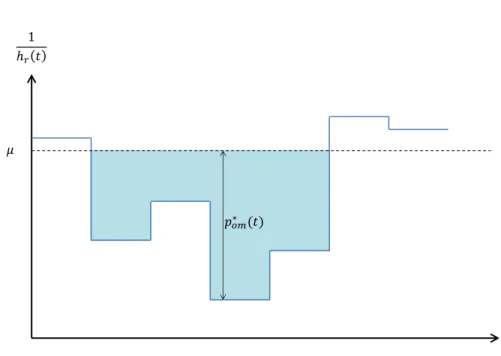
’W-shaped’ curve exhibits an interference classification into 5 in-terference regimes. . . 39 3.1 System Model: Transmission scheme . . . 54 3.2 Illustration of the water-filling concept: computing the water
level µ and the power strategy p∗om . . . 60 3.3 Instantaneous power strategies p(t) vs. Time Slot Index t, for
several scenarios of future knowledge - Q(0)B∆t = 100 and T = 25. . 66 3.4 Energy Performance vs. Q(0)B∆t - Q(0)B∆t ranging from 1 to 100 and
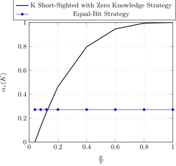
T = 25. . . . 67 3.5 αz(K) criterion vs. KT, Q(0)B∆t = 100 and T = 25. . . . 69
3.6 αs(K) criterion vs. KT, Q(0)
B∆t = 100 and T = 25. . . . 70
3.7 Energy Performance vs. Q(0)B∆t - Q(0)B∆t ranging from 1 to 200 and
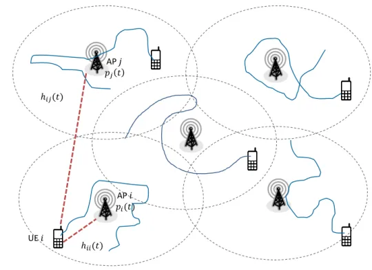
T = 25. . . . 71
4.1 System Model: N AP-UE pairs with mobile users, time-varying channels. . . 85 4.2 Transmission diagram for user i, by analogy from the previous
Figure 3.1 . . . 86 4.3 Illustrative example of the ’ping pong effect’ phenomenon. . . 93 4.4 Summary of the Mean Field Game. . . 102 4.5 Standard logistic sigmoid function, with φ = 50 and ρ = 1 . . . . 111
4.6 Optimal distribution of users m(t, Q) whose packet size at time slot t (x-axis) is Q (y-axis). Channel model 1 . . . 112 4.7 Optimal instantanous Mean Field power strategy p(t, Q) to be
used by any user whose packet size at time slot t (x-axis) is Q (y-axis). Channel model 1. . . 113 4.8 Instantaneous power strategies p(t) for 3 strategies, 3 different
initial packet sizes Q(0) = 20, 50, 100. Channel model 1. . . 114 4.9 Packet Sizes Evolutions Q(t) for 3 strategies, 3 different initial
packet sizes Q(0) = 20, 50, 100. Channel model 1. . . 115 4.10 Cumulated power cost C(t) =Pt
u=1p(u) for 3 strategies, 3
dif-ferent initial packet sizes Q(0) = 20, 50, 100. Channel model 1. . 116 4.11 Histogram of the final cumulated power cost E =PT
t=1p(t) over
the NM C independent Monte-Carlo Realizations, for the 3
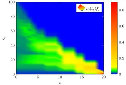
strate-gies. Channel model 1. . . 117 4.12 Optimal distribution of users ¯m(t, Q) whose packet size at time
slot t (x-axis) is Q (y-axis). Channel model 2. . . 120 4.13 Optimal instantanous Mean Field power strategy p(t, Q) to be
used by any user whose packet size at time slot t (x-axis) is Q (y-axis), by a user whose channel is h = 0.5. Channel model 2. . 121 4.14 Optimal instantanous Mean Field power strategy p(h, Q) to be
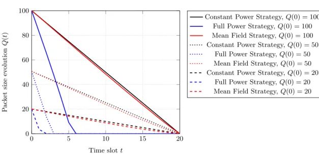
used by any user whose packet size at time slot t = 10 is Q (y-axis) and whose channel is h (x-axis). Channel model 2. . . . 122 4.15 Instantaneous power strategies p(t) for 3 strategies, 3 different
users. Channel model 2. . . 123 4.16 Packet Sizes Evolutions Q(t) for 3 strategies, 3 different users.
Channel model 2. . . 124 4.17 Cumulated power cost C(t) =Pt
u=1p(u) for 3 strategies, 3
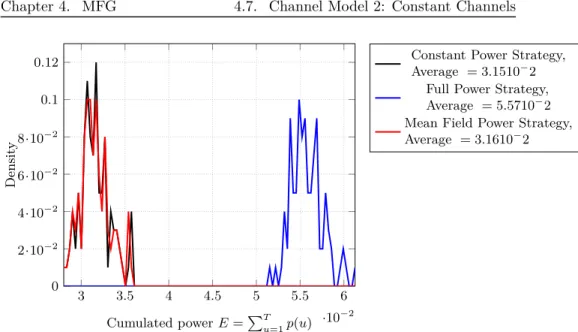
dif-ferent users. Channel model 2. . . 125 4.18 Histogram of the final cumulated power cost E =PT
t=1p(t) over
the NM C independent Monte-Carlo Realizations, for the 3
strate-gies. Channel model 2. . . 126 4.19 Channel evolution hij(t), with parameters C0 = 0.3 and f0 =
1000, resolution of 20 elements for [1, T ], T = 20. Channel model 3. . . 127
4.20 Optimal instantanous Mean Field power strategy p(h, Q) to be used by any user whose packet size at time slot t = 10 is Q (y-axis) and whose channel is h (x-(y-axis), at time slot t = 9 (Poor channel realizations, far from deadline). Channel model 3. . . 128 4.21 Optimal instantanous Mean Field power strategy p(h, Q) to be
used by any user whose packet size at time slot t = 10 is Q (y-axis) and whose channel is h (x-(y-axis), at time slot t = 12 (Good channel realizations, far from deadline). Channel model 3. . . 129 4.22 Optimal instantanous Mean Field power strategy p(h, Q) to be
used by any user whose packet size at time slot t = 10 is Q (y-axis) and whose channel is h (x-(y-axis), at time slot t = 16 (Poor channel realizations, close to deadline). Channel model 3. . . 130 4.23 Instantaneous power strategies p(t) for 3 strategies, initial packet
sizes Q(0) = 100, initial channel h(0) = 0.5. Channel model 3. . . 131 4.24 Cumulated power cost C(t) =Pt
u=1p(u) for 3 strategies, initial
packet size Q(0) = 100, initial channel h(0) = 0.5. Channel model 3. . . 132 4.25 Histogram of the final cumulated power cost E =PT
t=1p(t) over
the NM Cindependent Monte-Carlo Realizations, for the 3
strate-gies. Channel model 3. . . 133 4.26 Instantaneous power strategies p(t) for 3 strategies, initial packet
sizes Q(0) = 100, initial channel h(0) = 0.5. Channel model 4. . . 134 5.1 Generalized degrees of freedom, according to the α value. This
’W-shaped’ curve exhibits an interference classification into 5 in-terference regimes. . . 149 5.2 The 2-users Gaussian Interference Channel, considered during the
first half of this chapter. . . 150 5.3 Generalized degrees of freedom, according to the α value, for the
3 regimes interference classification. . . 153 5.4 A possible matching with one interferer from each coalition (M =
2, N = 3). Two coalitions of 3 UEs assigned to each AP have been represented. . . 161 5.5 One instance of the network deployment under investigation
-M = 2 APs and N = 20 UEs/AP. . . . 165 5.6 Histogram of the total spectral efficiencies of each scenario under
5.7 The M -users Gaussian interference channel, with M > 2. . . . . 167 5.8 An illustration of the proposed iterative Kuhn-Munkres algorithm.171 5.9 One instance of network deployment with M = 5 APs. For
sim-plicity, we consider coalitions of N = 7 interferers per AP. . . 173 5.10 Zoom on the histogram of the total spectral efficiencies of each
scenario under study, over NM C = 1000 independent
Monte-Carlo simulations. . . 174 5.11 Zoom on the histogram of the total spectral efficiencies of each
scenario under study, over NM C = 1000 independent
Monte-Carlo simulations. . . 175 6.1 The threefold optimization problem. The AP-UE assignment
comes as an additional layer to the previous optimization prob-lem, which only included matching of interferers and IC. . . 183 6.2 Illustrative example of ’Virtual Handover’: assigning the UE to
another AP, can provide a better spectral efficiency after inter-ference processing, even with a smaller SNR. . . 186 6.3 The maximum weight disjoint edges matching problem in a 2N
-complete graph. The red bold configuration is a possible disjoint matching, which matches interferers 1 and 2, 4 and 6, 3 and 5. . 193 6.4 Histogram plot of the performances of each scenario, for NM C =
1000 independent realizations (M = 2 interferers per group, N = 25 groups of interferers). . . 195 6.5 The general M -GIC considered in this section. . . . 198 6.6 Obtained spectral efficiency after interference processing Si(Ri, R−i),
for several values of Ri and fixed R−i. . . 199 6.7 Overview of the Genetic Algorithm. . . 206 6.8 Histogram plot of the performances of each scenario, for NM C =
1000 independent realizations (M = 10 interferers per group,
Introduction
1.1
Background and Motivations for Green
Wire-less Networks
1.1.1
Network Trends
With exponential increases in communication traffic, the Information and Com-munication Technology (ICT) industry currently accounts for 2% of worldwide carbon emissions, and that figure is expected to at least double over the next decade as more people seek to connect with each other and with more content in new, richer ways [1]. Even a 2% contribution to global emissions and energy consumption is significant: the network component of this represents some 250-300 million tons of carbon emissions, according to GreenTouch Green Measure [2]. Apart from the environmental concern, there is also an economical motiva-tion behind reducing the network power consumpmotiva-tion: For instance, it appeared that Vodafone’s global energy consumption for 2007-2008 was about 3000 GWh, which corresponds to emitting 1.45 million tons of CO2 and represents a mon-etary cost of several hundred million Euros [3]. More specifically, it represents a significant part of the operating expenses of a network operator: for exam-ple, in a mature European market, it even reaches 18% [3]. But while network traffic is growing exponentially and is doubling every two years, the revenues of the network operators are only growing annually at less than 10% [1]. For this reason, a critical challenge that is facing the ICT industry is how to ensure that the operating cost, that are expected to follow the exponential communication
traffic trend, can be reduced in order to keep pace with the slowly increasing revenues. Based on this context, over the past two decades, concepts like ’green communications’ have emerged and designing energy-efficient communication networks has become an important issue, in particular, to manage operating costs [4]. The ’green communication’ concept sets the aspiration of achieving a thousandfold improvement from 2010 levels in the future energy efficiency, over current designs for wireless communication networks [4, 5]. This challenge is also rendered nontrivial by the requirement to achieve this reduction without signif-icantly compromising the quality of service (QoS) experienced by the network users. In order to enhance the global energy efficiency of the network, several research directions for green wireless networks have been identified. Since most of the energy consumption of a mobile network comes from the wireless access, i.e. comes from the power cost at each Base Stations (BS) side in the net-work, it appears immediately that the greatest opportunity to reduce energy consumption is to improve the base stations deployment and energy efficiency [6]. Several research directions for Green Wireless Networks have been proposed in literature, among which:
• Radio Resource Management (RRM) energy-efficient techniques, such as power control, sleep modes, etc.
• Improvement of the network deployment efficiency
• Multi-antenna techniques, such as using large multiple antennas system, virtual multiple input multiple output (MIMO), beamforming or spatial multiplexing.
In this thesis, we focus mainly on the first two concepts, that we detail more extensively hereafter.
1.1.2
Research Directions for Green Wireless Networks
-Radio Resource Management, Cognitive -Radios and
Power Control
1.1.2.1 Radio Resource Management Techniques: Power Control and Sleep Mode
A first set of solutions suggests to enhance the energy efficiency of the network via Radio Resource Management (RRM) and power control techniques. In such
techniques, made possible by the emergence of concepts like Cognitive Radios [7], the objective consists of adapting the network transmissions settings, to the network context, in order to maximize a given utility function. In green wireless networks, the utility function to be considered is often the energy efficiency of the network or the users. Among the possible settings to be adapted, the trans-mission powers used at each base station often appears as the best candidate for two reasons. First, the operating power cost of the BS is in fact directly related to the transmission power [8], which is in turn related directly to the power consumption and the energy efficiency of the network. Second, the trans-mission powers are directly related to the interference patterns in the network: adapting the powers allows to regulate the interference in the network. This leads to power control problems, whose objective is to regulate the power, in order to provide each user an acceptable connection, while at the same time reducing the total power consumption of the network and limiting the interfer-ence [9, 10]. It is well known, in literature, that minimizing interferinterfer-ence using power control increases capacity, while reducing the power consumption at the same time [11, 9, 10]. Kandukuri and Boyd [12] also address both the mini-mization of transmitter power subject to constraints on outage probability and the minimization of outage probability subject to power constraints.
In practice, the power control approach can also aim at minimizing the power consumption of a base station, which can also be modeled with two parts. The first part describes the static power consumption, due to hardware cooling, the A/D conversion, the signal processing, etc. Depending on the load situation and the power consumption, a dynamic part adds to the static power [8]. It is observed that the static part is the main contribution to the base station power cost. As a consequence, turning the base station off, commonly referred to as sleep mode, when it is unused, might allow to save even more energy, as it almost completely negate the power cost of the base station [13, 14, 15]. In [16] for example, the authors then suggest to exploit this technique with high potential: they schedule transmissions in order to maximize the sleep time of the base station, thus greatly enhancing the energy savings.
1.1.2.2 Delay Tolerance and Future Knowledge: Proactive Delay-Tolerant Networks
At the same time, recent studies have also revealed that most of the network transmissions could be labeled as non-urgent: many mobile applications are
then ’delay-tolerant’, scheduling future transmissions can save power and thus money (often referred to as OPEX for Operational Expenditures): for example, a cell phone user might be willing to delay sending a non-urgent email mes-sage or download application updates for up to several hours if this allows to transmit over a low-cost interface [17, 18]. The system can then freely schedule its required transmission over the offered latency, in order to reduce the global power consumption required to complete this transmission. This is commonly referred to as the latency vs. energy-efficiency trade-off in literature [19] and it has led to the so-called concept of ’delay-tolerant networks’ [20, 21, 22].
In such delay-tolerant networks, the system is allowed to schedule its trans-mission and adapt its transtrans-mission settings, often the transtrans-mission powers at each BS, in order to optimize a given utility function, under a set of given constraints. Both the utility function and the constraints are usually used to model the satisfaction of the users in the network, and/or the satisfaction of the network operator. In [23, 24, 25], the author study the activation prob-lem which determines when a mobile will turn on in order to receive packets, and also address the transmission control problem, whose objective is to con-trol the total power cost. The conducted optimization allows to maximize the throughput of the system, while constraining the energy to be used. Moreover, the delay tolerance can also be used to allow the system to better handle the network congestion, as suggested in [20, 26, 27]: the network can then freely decide to transmit when the network resources are underused, thus limiting the congestion.
In addition to the delay tolerance, several recent works have also revealed that human behavior was highly and accurately predictable [28, 29]. The mobil-ity of a user in the network is often constrained by roads or streets, thus allowing for easily accurate short-term predictions on the user mobility [30, 31]. Coupling the prediction of the user mobility with radio maps, providing the expectation of the path loss perceived by a user at any geographical position, can lead to accurate predictions on the expected future link quality [32, 33, 34]. As a conse-quence, recent works have then looked forward to coupling scheduling techniques with future context predictions, in order to enhance the network performance leading to so-called proactive networks, as introduced in [35, 36, 37]. Significant diversity gains were analytically demonstrated, thus illustrating the significant potential benefit of proactive networks. In these papers [38, 39, 40] for example, the system is able to formulate predictions on the upcoming requests and user
mobility: by coupling it with a radio map giving measured reception quality at different locations, the system can then formulate predictions on the expected future transmission contexts. And based on these predictions, it then adapts its present transmission settings, in order to limit its own outage probability.
1.1.3
Single User Proactive Delay-Tolerant Transmissions:
a Toy Example for Convex Optimization
In the first half of this thesis, we investigate how the system might exploit an offered latency, when coupled with information about the upcoming transmis-sion context, that we refer to as ’future knowledge’. To do so, we first consider an illustrative toy example of a proactive delay-tolerant system. In Chapter 3 and as in [41, 42], we investigate a single user system, where one base station is enforced to complete a given data transmission before a given deadline, but is able to adapt its transmission power settings and aims at minimizing the total power consumption required to complete the transmission before the deadline. The system can freely adapt the power level to be used at the beginning of each time slot. The remaining packet size decreases according to an instantaneous rate which is a function of the SINR, i.e. a function of the transmission power used, the current channel realization during this time slot. We assume that the system has perfect knowledge of the channel realization that will occur during the whole duration of the present time slot, and can then adapt the transmission setting to be used to the current channel, as well as the remaining packet size and the number of remaining time slots until the deadline. We also consider that the system has a certain knowledge about the future transmission context, more specifically it has a certain knowledge about the future channel realiza-tions. The considered predictor is modeled as a Probability Density Function (PDF) that represents the prediction of the future channel realizations on each remaining time slot. The system can then adapt its current transmission power and instantaneous rate, based on both the present context and the expectation of the future transmission context.
In practice, defining the optimal power level to be used at the beginning of each time slot is equivalent to solving a power control problem, which consists of a mathematical optimization: the objective is to maximize or minimize a util-ity function (e.g. the energy cost, the energy efficiency,etc.) by systematically choosing the ’best’ set of parameters for this function (e.g. the transmission power, as the utility function directly relies on the transmission powers at the
base station). Most of the time, when facing power control and optimization problems, the problem turns out to be convex. We then may refer to the theory of convex optimization, for which the book of Boyd and Vandenberghe [43] is certainly one of the most cited and complete reference. In case of non-convexity, some papers either investigate how the problem can be assumed convex, or pro-pose specific algorithms to deal with these non-convex scenarios. In the general case, the optimal solution is attained by computing the Lagrangian associated with the optimization problem. The Lagrangian links the objective function to equality and inequality constraints functions by using Lagrange multipli-ers. Karush-Kuhn-Tucker(KKT) conditions [44] can then be used to derive the optimal solution to the problem. When not possible, the alternative solution consists of an iterative backward dynamic programming algorithm, that we also detail in this chapter [45].
When the system has perfect a priori knowledge of the future yet to come, i.e. knows a long time in advance the exact future channel realizations, the optimal strategy can be simply computed using a time water-filling algorithm, which is derived from the Karesh-Kuhn-Tucker conditions [44]. Water-filling based power allocation techniques have been widely presented [43, 46, 47] and investigated in the literature [48, 49, 50]. However, accessing a perfect knowledge about the future is an ideal scenario.
In this chapter, we propose to investigate several scenarios of future knowl-edge, ranging from a complete lack of knowledge to a perfect knowledge scenario and observe how the system may benefit from each scenario of future knowledge. The scenarios investigated in this chapter can be either:
• perfect knowledge: the system has perfect a priori knowledge about the exact future channel realizations. This is the best future knowledge scenario that the system can be given and leads to the optimal performance bound.
• zero knowledge: the system has no information about the future channel realizations. In this scenario, the system either transmits at a constant rate on each time slot (equal-bit scheduler), or it transmits assuming the worst possible channel realizations for each remaining time slot (which in the end leads to a min-max problem, that can be solved using the time water-filling algorithm as well).
com-pute the optimal power strategy to be used using the iterative backward dynamic programming algorithm.
• short-term perfect knowledge, with zero information about the
remaining time slots: in this scenario, we assume that the system can
perfectly predict the future channel realizations on a few upcoming time slots, but does not have any information about the remaining time slots. • short-term perfect knowledge, with statistical information about
the remaining time slots: in this scenario, we assume that the system
can perfectly predict the future channel realizations on a few upcoming time slots. The system is also given the channel statistics as future knowl-edge about the channel realizations on the remaining time slots.
The complete list of future knowledge scenarios is extensively detailed in Sec-tion 3.4. In each scenario, numerical simulaSec-tions provide good insights on how the system benefits from proactive resource allocation and each kind of future knowledge.
Through this simple illustrative example, we provide answers to the follow-ing three fundamental questions related to delay-tolerant networks and future knowledge:
• How can the system exploit some future knowledge? A possible way for the system to exploit this future knowledge relies on exploiting the power-efficiency latency trade-off. We model a delay-tolerant transmitter, and consider a power control optimization problem, where the objective is to minimize the global power consumption required for completing a fixed transmission before a given deadline. The transmitter is cognitive and can adapt its transmission power to the present transmission context, in real time. The decision process for the optimal power strategy is then affected by the present state (time remaining before deadline, packet size remaining,etc.) but is also able to take into account some piece of future knowledge about the future transmission context.
• Does future knowledge offer significant performance gains? The numerical simulations show that there is a significant gain between i) the zero knowledge scenario, which is the worst scenario of future knowledge, since the system does not know anything about the future transmission
context, and thus is lower performance bound; and ii) the perfect knowl-edge scenario, which is the best scenario of future knowlknowl-edge, since the system has perfect knowledge of the future at any time, and thus is the higher performance bound. Demonstrating that the gain was significant really mattered: if the performance gap had not been significant enough, then looking for future knowledge, and providing it to the system, so that it can exploit it via scheduling and proactive resource allocation would not have made sense. The performance gain would have been limited, and there would have been really little chance that this performance gain would have surpassed the cost of accessing and exploiting this future knowledge (commonly referred to as the ’cost of learning’). This chapter does not include details about how future knowledge might be acquired, nor does it define the cost of learning for every single future knowledge scenario. Nevertheless, a few details on this topic are discussed in Section 3.6. • What kind of future knowledge is really useful to the system?
The conducted analysis shows that the system may greatly benefit from partial future knowledge, and may almost reach the performance of the perfect knowledge scenario. More specifically, it turns out that a good statistical knowledge of the future context can offer significant perfor-mance gains. Also, it appears that a short-term knowledge (i.e. precise knowledge about the close future exclusively) can also provide significant performance gains.
1.1.4
Multi-user Proactive Delay-Tolerant Transmissions:
Multi-user Non-Cooperative Stochastic Games
In the second chapter (Chapter 4) of the first half of this thesis, we investigate the extension of the previous toy example to a multiuser scenario. We considerN ≥ 2 pairs of Base Stations and users, each BS is given the objective of
trans-mitting a given packet (whose initial size may vary from one pair to another) to its assigned user before a common deadline. Each BS can again adapt the power level to be used at the beginning of each time slot, as in the previous chapter. The problem complexifies, as we must now consider interference, which models the competition between users. At each user receiver side, the SINR term now includes an interference term that sums up how the instantaneous rate of one pair is affected by the other pairs power strategies. We have then N competitive
transmissions occurring, at the same time, and the BS have the same objective: completing a required transmission before a given deadline, at a minimal cumu-lated power cost. And each user decides at the beginning of each time slot, the optimal power strategy to be used for transmission, based on the current con-text (remaining packet size, remaining time slots, present channels realizations between all BS and users) and the expectation of the future channel realizations, which are modeled according to an Itô process [51].
In the considered multiuser competitive scenario, computing the optimal power strategy to be used by each user, at the beginning of each time slot re-lies on game theory, more specifically non-cooperative stochastic game theory, because of the Itô process. Game theory is a mathematical framework, born in the field of economics [52, 53], that investigates the strategical interactions between competing, rational decision takers known as players. Broadly speak-ing, game theory can be divided into cooperative game theory, in which players are free to form coalitions to achieve a common goal, and non-cooperative game theory, in which each player competes with each other to achieve a selfish goal [53]. In non-cooperative game theory, the most widely used solution concept is the famous notion of Nash Equilibrium (NE) [54, 53] and its refinements. A NE is an equilibrium state of the game in which no player can improve its utility by a unilateral deviation: a NE configuration satisfies all the players, as they do not feel like they could improve their situation by changing independently their current strategy, thus leading to a stable configuration.
When analyzing the NE configuration of the previously mentioned game, our conducted analysis reveals that two approaches can be considered, in the general case:
• The Nash Equilibrium configuration can be accessed by solving a set of N couple Partial Differential Equations (PDE), namely N coupled Hamilton-Jacobi-Bellman equations, as suggested in [53]. Solving a set of N coupled PDEs can rapidly become complicated, especially when the number of partial derivatives corresponds to all the possible transmission settings (all the cross channels between all BS and users, and the remaining packet sizes for each pair).
• When no stochasticity is considered, the Nash Equilibrium configuration can be approached by an iterative time water-filling algorithm [55, 56, 57, 58, 59], where each BS can adapt, its individual power strategy to the
transmission context and the other BS current power strategies. However, when a BS adapts it power strategy, the interference pattern perceived by the other users in the system is reset and the other BS might no longer be satisfied with their current power strategy, and the readjustments will again reset the interference pattern of the system. Because of this ’ping-pong effect’ between players, the iterative process is demonstrated to con-verge to a fixed point, which corresponds to the NE configuration [55]. However, the computation time required to observe such a convergence tends to explode when the number of users in the system N increases, rendering large problems untractable [60].
Both approaches appear complex because each player action has an immediate impact on the other players perceived performance. The decisions made by a player must then take into account the anticipation of the other users actions. This phenomenon dramatically increases the inherent mathematical complexity of the problem, especially when the number of users N grows large, but several solutions allow to bypass the complexity of the problem:
• Focus on scenarios where the number of users N remains small enough, so that we can solve the set of N coupled PDEs. This solution is however extremely limited in our scenario, as the set of equations becomes already extremely complex to solve, even for N = 3.
• Focus on scenarios where the evolution of the channels is simpler than a stochastic model. If the channel does not have a stochastic part (i.e. the channel evolution is perfectly estimated), the iterative time water-filling algorithm can be used to approach the NE configuration. However, we must keep in mind that the number of players in the system N must remain relatively small, so that the computation time necessary to observe the converge of the iterative algorithm to a fixed point, remains acceptable. In scenarios where the channels are constant wrt to time, as in [61] (i.e. both the deterministic and stochastic parts are equal to zero), the optimal power strategies can be simply computed by solving a set of N linear equations.
• A heuristic suboptimal power strategy can also be considered. Such a heuristic strategy is simple to compute, but is by definition suboptimal. In this chapter, we investigate two heuristics: a constant power heuristic (the power strategies are necessarily constant wrt time), and a full-power
heuristic (which transmits at maximal power and stops when the trans-mission is completed).
Several solutions exist, but none of them allows to solve the problem in the stochastic configuration, with a large number of players N . This is quite prob-lematic, especially since today’s trend is to dense large heterogeneous networks, as detailed in Section 1.1.6.1.
1.1.5
Mean Field Games
We have demonstrated in the previous section, that the inherent mathematical complexity related to multi-user non-cooperative stochastic games could render the problem untractable, especially when the number of users grows large. The cause for this complexity is the high number of interactions between the N users in the system, N being supposed large. However, when the number of users grows large, the impact of a single player action on its neighbors might becomes negligible at the large scale of the system. Also, we might observe symmetries between users: same objective functions, same sets of actions, same evolution models, etc. It is then possible to simplify the problem, by exploiting those symmetries when the number of users N grows large [62]. The Mean Field Theory, relies on these ideas and allows to approximate a multi-user stochastic game and turn a N users game into a more tractable equivalent game, called a Mean Field Game (MFG), as it was introduced by Lasry and Lions [63, 64, 65]. This equivalent Mean Field Game presents the advantage of having a 2-body complexity only, compared to the N -body complexity of the initial multi-user non-cooperative stochastic game.
Several recent papers have implemented such a Mean Field framework, in order to simplify the resolution of multi-user stochastic games. For example, in [66, 67], every user has to adapt their strategies to the quality of their environ-ment( link quality, channel, etc.), while ensuring a minimal SINR constraint. In [68], a similar and interesting analysis is provided, with an application of the MFG tools, into the topic of electrical vehicles in the smart grids. In [69, 61], the players are transmitters, who adapt their transmission powers to the qual-ity of their link with the receiver, the strategies of the other users, and their battery level, while ensuring a SINR constraint. In a similar way, we turn an untractable N users stochastic game into a MFG and study the Mean Field Equilibrium of the new-built game. The Mean Field Equilibrium leads to the
mean field optimal set of power strategies, that will be used for approximate the optimal strategies of the original N users stochastic game.
In Chapter 4, we propose to exploit the recent Mean Field Games advances, in order to transition our initial multi-user non-cooperative stochastic game into an equivalent Mean Field Game. The conducted analysis reveals how the Mean Field Equilibrium can be computed, in order to define a common power strategy to be used by any user in the initial multi-user non-cooperative stochastic game, in any configuration (time, remaining packet size, channels). The returned mean field power strategy approaches the optimal power strategy when it can be com-puted, for example in scenarios where there are no variations on the channels wrt time. We study the performance of the mean field power strategy, for sev-eral channel models (from the constant channel case to the complete stochastic problem) and we provide numerical simulations assessing the performance of the investigated optimal MFG, compared to a set of reference strategies (iterative time water-filling when possible, full-power heuristic strategy, constant power heuristic strategy).
Numerical results reveal that the Mean Field power strategy closely ap-proaches the optimal power strategy, when it can be explicitly computed (i.e. constant channel scenarios). In scenarios where the channel become time-varying with no stochasticity, the optimal power strategy can not be simply computed for large dimension scenarios. Only constant power heuristic and full-power heuristic strategies are considered, and it is observed that the Mean Field power strategy outperforms both heuristics, revealing a twofold gain, that can be decomposed with one performance gain due to the latency and one performance gain due to the future knowledge. For this reason, proactive delay-tolerant frameworks appear to offer a significant energy gain, confirming the importance of the concept in Green Wireless Networks. It must noted that the future knowledge does not provide any gain, when the channels are not time-varying, as the equal-bit scheduler could have been used to compute the optimal power strategy, without any future knowledge, which confirms what has been observed in the previous chapter. Finally, we study the impact of the stochas-tic part on the Mean Field power strategy, and reveal that the uncertainty of the future strongly affects the optimal Mean Field power strategies: the system becomes more cautious about the future and might instead prefer to transmit notably earlier in advance, thus becoming less able to exploit the offered la-tency, as it did with the zero knowledge scenario, in Chapter 3. be decomposed
with one performance gain due to the latency and one performance gain due to the future knowledge. For this reason, proactive delay-tolerant frameworks appear to offer a significant energy gain, confirming the importance of the con-cept in Green Wireless Networks. It must noted that the future knowledge does not provide any gain, when the channels are not time-varying, as the equal-bit scheduler could have been used to compute the optimal power strategy, without any future knowledge, which confirms what has been observed in the previous chapter. Finally, we study the impact of the stochastic part on the Mean Field power strategy, and reveal that the uncertainty of the future strongly affects the optimal Mean Field power strategies: the system becomes more cautious about the future and might instead prefer to transmit notably earlier in ad-vance, thus becoming less able to exploit the offered latency, as it did with the zero knowledge scenario, in Chapter 3.
1.1.6
Research Directions for Green Wireless Networks
-Enhancing the Deployment Efficiency and
Bottle-necks
1.1.6.1 Enhancing deployment efficiency: towards large heteroge-neous networks
A second set of solutions for green networking relies on improving the network deployment, by densifying it with relays, small cells, femto/pico-cells, leading to the so called dense heterogeneous networks [70, 71, 72]. This first set of solutions relies on the well-known fact that cell-size reduction is the simplest and most effective way to increase the global network capacity, by enhancing the spatial reuse [73]. Also, due to their short transmit-receive distance, small cells can greatly lower transmit powers, prolong handset battery life, and achieve a higher signal-to-interference-plus-noise ratio (SINR), thus resulting in a better spectral efficiency [72]. Improving the network deployment efficiency then leads to win-win solutions for network operators, as they enhance the global network capacity, while reducing at the same time the base station power costs.
However, it must be noted that such heterogeneous networks are more com-plex to handle for the operators, due to their large number of elements and their multi-tier topology structure, consisting of a first tier with high power large coverage macrocells and a second tier with low power small coverage pico/femto/small cells. The multiplicity of wireless communication systems
in-creases the spectrum pollution due to interference. As a consequence of the large number of Base Stations transmitting in a same geographical area, the in-band interference, which models the interactions between the different elements of the networks sharing the same spectral resources, has become an important issue to be addressed in the heterogeneous networks.
1.1.6.2 Interference, The Universal Enemy
In the heterogeneous networks, the interference is classically perceived at each receiver side as the enemy. The classical approach treats interference, due to concurrent transmissions from other elements of the network using the same spectral resources, as an additional source of noise. For reliable transmissions to occur, the interference, which is classically treated as an additive source of noise, is perceived as an enemy. For this reason, it must be ideally avoided or at least strongly limited, in order to guarantee a good SINR, and a good spectral efficiency after interference processing. In order to cope with interfer-ence, two sets of techniques can be considered: techniques that aim at avoiding interference and techniques that aim at keeping the interference limited.
When attempting to avoid interference, the most common and simple ap-proach consists of orthogonalizing transmissions, by enforcing the different el-ements of the network to transmit using different spectral resources. Several well-known resource allocation techniques have been proposed to achieve such orthogonalization, by simply separating signals in time, frequency, space or code: Time/Frequency Division Duplex (TDD/FDD), Time/Frequency Division tiple Access techniques (TDMA/FDMA), Orthogonal Frequency Division Mul-tiple Access (OFDMA) Code/Space Division MulMul-tiple Access (CDMA/SDMA) [74, 75]. However, such orthogonal resource allocation can not be met in dense networks, since the set of available resources might not be large enough to allo-cate exclusive resource blocks to each element in the network. Moreover, such orthogonal allocation techniques lead to poor spectral efficiencies and drives the system to a drastic suboptimal spectral efficiency operating point.
Due to the large number of elements in the network, and the limitation of spectral resources, the orthogonalization, even though simple, might not always be the best option. When the elements in the network share the same spectral resources, their transmission is limited by in-band interference. Nevertheless, resources can be shared and reused in a smart fashion, as long as we manage to mitigate the in-band interference. Such interference management is enabled by
partial or full orthogonalization between competing interferers, as proposed by frequency reuse or graph coloring [76, 77, 78].
A second set of techniques, which allows interference to remain limited, so that reliable and efficient transmissions can occur, relies on the previously men-tioned power control approaches. The approach consists of carefully adapting the transmission powers, so that interference remains under a target limit: the system carefully balances power budgets allocation among interfering sources, as it will be detailed in the first half of the thesis, or in multiple papers in litera-ture [79, 10, 12, 11]. However, in order to solve such optimization problems and find optimal transmission strategies for every user in the system, we have to find an equilibrium configuration. When facing this problem, we demonstrated that this may involve a high mathematical complexity, especially when the system dimensions become large [80, 81, 60], as we must take into account all the one user to one user interactions, which is modeled by the interference perceived at each receiver side.
1.1.6.3 Is Interference Friend or Foe ? Interference Classification
Previously mentioned methods always assume that interference will be processed as an additive source of noise. In that sense, the mentioned methods do not profit of the recent advances in the domain of information theory, showing that interference might not necessarily be an opponent, but may become, in fact, an ally, especially in cases where the interference becomes strong, which is com-monly identified as an interference badly compromising the transmission. In practice, Carleial [82] and, later on, Han & Kobayashi [83] have demonstrated that it was possible to exploit intrinsic properties of the interference, in order to process interference differently and obtain notably higher rates after interfer-ence processing. The observation, which allowed the trick to happen, consisted of observing that interference was not just an additive source of noise. In fact, Carleial suggested that, in scenarios of strong interference, the strong limitation of the rate was not due to theoretical limitations, but was instead due to the communications techniques employed for processing interference. He proposed an interference processing technique, which first aims at decoding the strong interference in presence of the primary signal, and then subtracts the decoded interference from the received signal, leaving it with no trace of interference. The main concept behind this idea is commonly referred to as Successive In-terference Cancellation (SIC) [82] and is considered as the optimal inIn-terference
processing technique for strong interference scenarios, as it allows to remove completely the strong interference. Based on this observation, it immediately appeared that a single interference mitigation technique, namely the noisy pro-cessing, could not perform well for all the possible scenarios of interference, ranging from weak to strong interference.
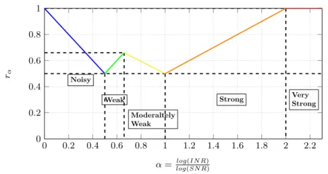
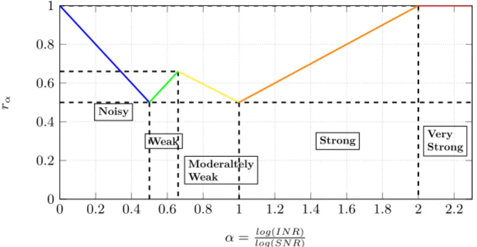
As a matter of fact, exploiting additional interference mitigation techniques, such as SIC, has been recently perceived as a promising feature for 5G net-works [84]. It also inspired the net-works of Etkin & Tse [85], who investigated the different interference mitigation techniques from a single user point of view and their spectral efficiencies after interference processing. They defined the SNR/INR configurations for which each interference mitigation technique was the most-suited technique. In a two-user Gaussian interference channel, they proved that for any pair (R1, R2) in the interference capacity region, the consid-ered schemes were able to achieve the spectral efficiencies pair (R1−1, R2−1) for any values of the channel parameters (i.e. SNR and INR). Basically, this means that the presented schemes in this paper were able to achieve spectral efficiencies within 1 bit/s/Hz of the capacity of the interference channel. Five interference regimes, i.e. interference mitigation techniques were identified, each of them being the most-suited technique in a given region of α, which was de-fined as α = log(SN R)log(IN R). In the following we recall the presented classification of the interference mitigation techniques proposed by Etkin and Tse, as the ’5-Regimes Interference Classification’. We represented the 5 ’5-Regimes and their performance, illustrated by the well-known ’W-shaped’ Figure 2.1.
This ’5-Regimes interference classification’ was later simplified by Abgrall [86, 87], who proposed a simplified version of this classification, reducing the classification to only 3 regimes. The interference may either be treated as an additive source of noise if it is perceived as weak, exploited and canceled via SIC if it is perceived as strong, or simply avoided via orthogonalization, if it is neither perceived as strong or weak. To justify the simplification, Abgrall suggested that even if some of them perform very well theoretically, they may suffer from infeasibility in practice because of excessive computational complexity or strict operating assumptions. For example, simultaneous superposition coding is up to now too complex to be used in practice. For this reason, Abgrall favored the use of techniques which can be implemented in practical systems without stringent limitations. More details about each classification and the considered classification regimes will be detailed in a short tutorial, in Section 5.2.
0 0.2 0.4 0.6 0.8 1 1.2 1.4 1.6 1.8 2 2.2 0 0.2 0.4 0.6 0.8 1 Noisy Weak Moderaltely Weak Strong Very Strong α = log(SN R)log(IN R) rα
Figure 1.1: Generalized degrees of freedom, according to the α value. This ’W-shaped’ curve exhibits an interference classification into 5 interference regimes.
In the second half of the chapter, we propose to address the dual problem to the previous power control approach, namely, we look forward to optimizing the spectral efficiency of the system, under a fixed power configuration. In this part, we propose to focus on the interference, which degrades the quality of the transmissions in the network. Similarly to recent works that have proposed to exploit interference classification (e.g. [88, 89]), we propose an interference classification based approach in Chapter 5, that enhances the system network performance, by finding the optimal way to process interference, thus exploit-ing the inherent properties of interference. To do so, we first consider a RRM problem, in a 2-users Gaussian Interference Channel. The system deals with the perception of the interference at each receiver side and aims at maximiz-ing the total spectral efficiency, assummaximiz-ing the interference is treated accordmaximiz-ing to the 3-regimes classifier defined by Abgrall. More specifically, we propose to adapt the perceived robustness of transmission at each receiver side, by adapting the spectral efficiencies and the reliability of the transmissions, to the channel context. This way, we reduce the complexity of the optimization problem, by only allowing changes on the interference perception of each user. We leave unchanged the short-term power configuration and interference patterns, since it causes an avalanche of changes in the network [60, 86]: such an approach directly tackles the ’ping pong effect’ we described earlier and the associated computational complexity observed in the iterative processes and instead allows for low-complexity optimization. The analysis of the optimization problem