Performance Bounds for Lambda Policy Iteration and Application to the Game of Tetris

Similarly to the 1-dimensional case, we shall prove the compactness of functions with equi- bounded energy by establishing at first a lower bound on the functionals E h.. Thanks to

In this study, we provide new exponential and polynomial bounds to the ratio functions mentioned above, improving im- mediate bounds derived to those established in the

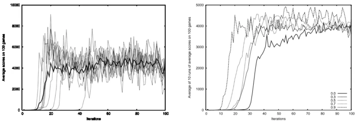
Even though the theory of optimal control states that there exists a stationary policy that is optimal, Scherrer and Lesner (2012) recently showed that the performance bound of

The documents may come from teaching and research institutions in France or abroad, or from public or private research centers.. L’archive ouverte pluridisciplinaire HAL, est

In trials of CHM, study quality and results depended on language of publication: CHM trials published in English were of higher methodological quality and showed smaller effects

Spruill, in a number of papers (see [12], [13], [14] and [15]) proposed a technique for the (interpolation and extrapolation) estimation of a function and its derivatives, when

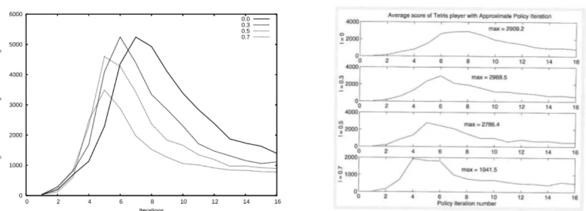
For the last introduced algorithm, CBMPI, our analysis indicated that the main parameter of MPI controls the balance of errors (between value function approximation and estimation

Shi, Bounds on the matching energy of unicyclic odd-cycle graphs, MATCH Commun.. Elumalai, On energy of graphs,