HAL Id: hal-03047875
https://hal.archives-ouvertes.fr/hal-03047875
Submitted on 10 Dec 2020
HAL is a multi-disciplinary open access
archive for the deposit and dissemination of
sci-entific research documents, whether they are
pub-lished or not. The documents may come from
teaching and research institutions in France or
abroad, or from public or private research centers.
L’archive ouverte pluridisciplinaire HAL, est
destinée au dépôt et à la diffusion de documents
scientifiques de niveau recherche, publiés ou non,
émanant des établissements d’enseignement et de
recherche français ou étrangers, des laboratoires
publics ou privés.
from tropospheric ozone using TES satellite observations
K. Bowman, D. Shindell, H. Worden, J.F. Lamarque, P. Young, D. Stevenson,
Z. Qu, M. de la Torre, D. Bergmann, P. Cameron-Smith, et al.
To cite this version:
K. Bowman, D. Shindell, H. Worden, J.F. Lamarque, P. Young, et al.. Evaluation of ACCMIP outgoing
longwave radiation from tropospheric ozone using TES satellite observations. Atmospheric Chemistry
and Physics, European Geosciences Union, 2013, 13 (8), pp.4057-4072. �10.5194/acp-13-4057-2013�.
�hal-03047875�
Atmos. Chem. Phys., 13, 4057–4072, 2013 www.atmos-chem-phys.net/13/4057/2013/ doi:10.5194/acp-13-4057-2013
© Author(s) 2013. CC Attribution 3.0 License.
EGU Journal Logos (RGB)
Advances in
Geosciences
Open Access
Natural Hazards
and Earth System
Sciences
Open AccessAnnales
Geophysicae
Open AccessNonlinear Processes
in Geophysics
Open AccessAtmospheric
Chemistry
and Physics
Open AccessAtmospheric
Chemistry
and Physics
Open Access DiscussionsAtmospheric
Measurement
Techniques
Open AccessAtmospheric
Measurement
Techniques
Open Access DiscussionsBiogeosciences
Open Access Open Access
Biogeosciences
Discussions
Climate
of the Past
Open Access Open Access
Climate
of the Past
Discussions
Earth System
Dynamics
Open Access Open Access
Earth System
Dynamics
DiscussionsGeoscientific
Instrumentation
Methods and
Data Systems
Open Access
Geoscientific
Instrumentation
Methods and
Data Systems
Open Access DiscussionsGeoscientific
Model Development
Open Access Open Access
Geoscientific
Model Development
DiscussionsHydrology and
Earth System
Sciences
Open AccessHydrology and
Earth System
Sciences
Open Access DiscussionsOcean Science
Open Access Open Access
Ocean Science
Discussions
Solid Earth
Open Access Open Access
Solid Earth
Discussions
Open Access Open Access
The Cryosphere
Natural Hazards
and Earth System
Sciences
Open Access
Discussions
Evaluation of ACCMIP outgoing longwave radiation from
tropospheric ozone using TES satellite observations
K. W. Bowman1, D. T. Shindell2, H. M. Worden3, J.F. Lamarque3, P. J. Young4, D. S. Stevenson5, Z. Qu6,
M. de la Torre1, D. Bergmann7, P. J. Cameron-Smith7, W. J. Collins8, R. Doherty5, S. B. Dalsøren9, G. Faluvegi2, G. Folberth10, L. W. Horowitz11, B. M. Josse12, Y. H. Lee2, I. A. MacKenzie5, G. Myhre9, T. Nagashima13, V. Naik15, D. A. Plummer16, S. T. Rumbold10, R. B. Skeie9, S. A. Strode17, K. Sudo14, S. Szopa18, A. Voulgarakis20, G. Zeng19, S. S. Kulawik1, A. M. Aghedo21, and J. R. Worden1
1Jet Propulsion Laboratory-California Institute of Technology, Pasadena, CA, USA
2NASA Goddard Institute for Space Studies and Columbia Earth Institute, New York, NY, USA 3National Center for Atmospheric Research,Boulder, Colorado, USA
4Lancaster Environment Centre, Lancaster University, Lancaster, UK 5School of GeoSciences, The University of Edinburgh, Edinburgh, UK 6Raytheon Intelligence & Information Systems, Pasadena, CA USA 7Lawrence Livermore National Laboratory, Livermore, CA, USA 8Department of Meteorology, University of Reading, Reading, UK
9Center for International Climate and Environmental Research, Oslo, Norway 10Met Office, Hadley Centre, Exeter, UK
11NOAA Geophysical Fluid Dynamics Laboratory, Princeton, NJ, USA
12GAME/CNRM, M´et´eo-France, CNRS – Centre National de Recherches M´et´eorologiques, Toulouse, France 13National Institute for Environmental Studies, Tsukuba, Japan
14Graduate School of Environmental Studies, Nagoya University, Nagoya, Japan 15UCAR/NOAA Geophysical Fluid Dynamics Laboratory, Princeton, NJ, USA
16Canadian Centre for Climate Modeling and Analysis, Environment Canada, Victoria, British Columbia, Canada 17NASA Goddard Space Flight Center and Universities Space Research Association, Columbia, Maryland, USA 18Laboratoire des Sciences du Climat et l’Environnement, Gif-sur-Yvette, France
19National Institute of Water and Atmospheric Research, Lauder, New Zealand 20Department of Physics, Imperial College London, London, UK
21Civil and Environmental Engineering,Rice University, Houston, TX, USA
Correspondence to: K. W. Bowman ([email protected])
Received: 31 July 2012 – Published in Atmos. Chem. Phys. Discuss.: 11 September 2012 Revised: 5 March 2013 – Accepted: 14 March 2013 – Published: 18 April 2013
Abstract. We use simultaneous observations of tropospheric
ozone and outgoing longwave radiation (OLR) sensitivity to tropospheric ozone from the Tropospheric Emission Spec-trometer (TES) to evaluate model tropospheric ozone and its effect on OLR simulated by a suite of chemistry-climate models that participated in the Atmospheric Chemistry and Climate Model Intercomparison Project (ACCMIP). The en-semble mean of ACCMIP models show a persistent but mod-est tropospheric ozone low bias (5–20 ppb) in the
South-ern Hemisphere (SH) and modest high bias (5–10 ppb) in the Northern Hemisphere (NH) relative to TES ozone for 2005–2010. These ozone biases have a significant impact on the OLR. Using TES instantaneous radiative kernels (IRK), we show that the ACCMIP ensemble mean tropospheric ozone low bias leads up to 120 mW m−2OLR high bias lo-cally but zonally compensating errors reduce the global OLR high bias to 39 ± 41 m Wm−2relative to TES data. We show that there is a correlation (R2= 0.59) between the magnitude
of the ACCMIP OLR bias and the deviation of the ACCMIP preindustrial to present day (1750–2010) ozone radiative forcing (RF) from the ensemble ozone RF mean. However, this correlation is driven primarily by models whose absolute OLR bias from tropospheric ozone exceeds 100 m Wm−2. Removing these models leads to a mean ozone radiative forc-ing of 394 ± 42 m Wm−2. The mean is about the same and the standard deviation is about 30 % lower than an ensemble ozone RF of 384 ± 60 m Wm−2 derived from 14 of the 16 ACCMIP models reported in a companion ACCMIP study. These results point towards a profitable direction of combin-ing satellite observations and chemistry-climate model sim-ulations to reduce uncertainty in ozone radiative forcing.
1 Introduction
Tropospheric ozone plays a central role in both atmospheric chemistry and climate. Due to significant increases in an-thropogenic emissions of its precursors since preindustrial times, tropospheric ozone has the third highest impact as an anthropogenic greenhouse gas in terms of radiative forcing, 350 [250–650] m Wm−2(Forster et al., 2007), but is distin-guished from other greenhouse gases by having significant spatial and temporal heterogeneity due to its relatively short lifetime. Ozone is an essential part of the oxidative capac-ity of the troposphere, both as an oxidant in its own right, but especially as a precursor of the hydroxyl radical (OH) (Wang and Jacob, 1998; Voulgarakis et al., 2013). Reaction with OH controls the chemical lifetime of many species in the atmosphere, including methane, providing a link between ozone concentrations and the global warming potential of methane (Shindell et al., 2005, 2009). In addition, changes in climate can affect the chemistry of ozone, including in-creasing the rate of OH production due to higher water va-por concentrations with warming temperatures, that will have impacts for methane and other gases, e.g., (Stevenson et al., 2006). Uncertainties in these processes impact knowledge of preindustrial ozone concentrations, the evolution of ozone, and present-day distributions. These factors contribute to the broad range of radiative forcing estimates in the IPCC.
Ozone can also indirectly affect the climate through the carbon and hydrological cycles. As it is a phytotoxin, in-creases in ozone can reduce global primary productivity and therefore the CO2 uptake by biota (plants, forests),
poten-tially leading to an indirect forcing of a similar magnitude to the direct ozone forcing (Sitch et al., 2007; Collins et al., 2010). These interactions have yet to be explored across a suite of models.
Studies since the Intergovernmental Panel on Climate Change (IPCC) Fourth Assessment Report (AR4) have found that changes in short-lived species, including tropo-spheric ozone, are expected to have a significant impact on global temperatures, especially over the Northern
Hemi-sphere (Levy et al., 2008; Shindell et al., 2008). In particular, by 2050, Short-Lived Climate Forcing (SLCF) agents could be responsible for up to 20 % of simulated global mean an-nually averaged warming and up to 40 percent of the total projected summertime warming in the central United States from 2050–2100 (Levy et al., 2008). However, the contribu-tion of short-lived species to simulated changes in global-mean surface temperature can have a strong dependence on both the SLCF magnitude and spatial distribution (Shindell and Faluvegi, 2009). These factors have been the impetus for policy formulation that mitigates both air quality and global warming, (West et al., 2006, 2007; van Vuuren et al., 2006; Wallack and Ramanathan, 2009; Ramanathan and Xu, 2010; Shindell et al., 2013) with the concomitant need for accurate measurements and model results.
The Atmospheric Chemistry and Climate Model Inter-comparison Project was initiated to complement the Climate Model Intercomparison Project, Phase 5 (CMIP5) (Taylor et al., 2011) by focusing on the coupling of chemically ac-tive atmospheric constituents with climate both historically and in the future (Lamarque et al., 2013). A suite of state-of-the-art chemistry-climate models were driven by common emissions and comparable boundary conditions over differ-ent time periods from preindustrial to presdiffer-ent-day. In ad-dition, simulations of future climate were calculated using emissions derived from Representative Concentration Path-way (RCP) scenarios (van Vuuren et al., 2011). This ap-proach can help quantify the role of SLCF in past and future climate response across a range of models, which was diffi-cult to do previously (Shindell and Lamarque, 2009). Conse-quently, ACCMIP will be a valuable resource for the IPCC AR5.
Furthermore, a constellation of satellites that can observe a number of trace gas constituents are now available with global coverage and data records of sufficient length to be useful for the evaluation of ACCMIP simulations. Expand-ing from the analysis of Aghedo et al. (2011b), we evaluate how ACCMIP tropospheric ozone bias effects OLR bias us-ing global, simultaneous observations of tropospheric ozone and sensitivity of OLR to tropospheric ozone from the Tropo-spheric Emission Spectrometer, which was launched aboard the NASA Aura spacecraft in 2004 (Beer, 2006), using data collected from 2005–2010. TES does not measure the full OLR but does measure spectral radiances in the 9.6 mi-cron ozone band. However, tropospheric ozone has by far the strongest infrared absorption in the 9.6 micron band (Clough and Iacono, 1995). Consequently, the impact of tropospheric ozone on OLR bias can be computed from the 9.6 micron ozone band alone. We apply TES Instantaneous Radiative Kernels (IRK) to the ACCMIP tropospheric ozone bias in order to relate changes in the vertical structure of tropo-spheric ozone to changes in OLR (δOLR) at the top-of-the-atmosphere (TOA). The TES IRK quantifies the sensitiv-ity of OLR to changes in the vertical distribution of tropo-spheric ozone for each satellite observation, accounting for
the effects of temperature, water vapor and effective cloud properties that are simultaneously estimated (Worden et al., 2011). These corresponding state parameters largely deter-mine atmospheric opacity and therefore control the magni-tude of the IRK. Consequently, we quantify the change in OLR due to ACCMIP tropospheric ozone bias referenced against the observed atmospheric state as opposed to a model simulated atmospheric state.
We then explore the implications of ACCMIP OLR bi-ases from tropospheric ozone on ozone radiative forcing (RF), which is defined as the net change in irradiance at the tropopause after stratospheric temperature adjustment due to changes in ozone concentrations from preindustrial to present day (Forster et al., 2007). Ozone RF is depen-dent on a number of factors, including preindustrial emis-sions, background concentrations (through lightning-derived NOx and stratospheric input), present-day concentrations, at-mospheric radiative transfer, chemical mechanisms, and the physical climate (e.g. clouds, temperature, humidity). Uncer-tainties in these processes potentially could lead to biases in present day OLR. Hence, we investigate whether ACCMIP ozone RF is correlated with ACCMIP δOLR.
2 Tropospheric emission spectrometer
Launched in July 2004, the NASA EOS Aura platform is in a polar, Sun-synchronous orbit with an equator crossing time of 13:40 and 02:29 local mean solar time for ascending and descending orbit paths, respectively. The Tropospheric Emis-sion Spectrometer (TES) is a Fourier Transform Spectrome-ter (FTS) that measures spectrally-resolved outgoing long-wave radiation of the Earth’s surface and atmosphere at fre-quencies between 650–2250 cm−1with unapodized spectral resolution of 0.06 cm−1 (Beer, 2006). This spectral resolu-tion is sufficient to resolve pressure-broadened IR absorpresolu-tion lines in the troposphere and allows TES to estimate simulta-neous vertical profiles of ozone, water vapor, carbon monox-ide, methane, deuterated water vapor as well as atmospheric temperature. Previous studies used these profiles under clear-sky scenes to estimate the greenhouse gas effect from upper tropospheric ozone to be 0.48 ± 0.14 Wm−2(Worden et al., 2008). Effective cloud pressure and optical depth, surface temperature and land emissivity are also derived from TES spectral radiances, which allows TES to perform ozone re-trievals in all-sky conditions (Eldering et al., 2008). Algo-rithms for radiometric calibration (Worden et al., 2007), re-trieval of atmospheric parameters (Bowman et al., 2006), and error characterization (Worden et al., 2004) along with cloud property retrievals (Kulawik et al., 2006) have been described previously. The TES forward model used for com-puting spectral radiances and Jacobians (Clough et al., 2006) is based on LBLRTM (line-by-line radiative transfer model), which has been used as the basis for a number of radiative transfer models in climate models (Forster et al., 2011). TES
radiances have been compared to other satellite and aircraft data (Shephard et al., 2008). There is no detectable trend in residual spectral radiances (observed minus calculated) from 2005–2009 to within 0.6 K (Connor et al., 2011). Previous validation studies of the TES ozone V002 product indicate ozone profiles are biased high in the troposphere (≈15 %) relative to ozonesondes (Nassar et al., 2008) and aircraft data (Richards et al., 2008) while total ozone columns are biased high by about 10 DU relative to OMI measurements (Oster-man et al., 2008). The optimal estimation technique used op-erationally on TES data provides formal uncertainties (Bow-man et al., 2002, 2006). These uncertainty estimates were tested by comparisons with northern latitude ozonesondes re-ported in Boxe et al. (2010), which showed that formal mea-surement and species interference errors were consistent with empirical calculations.
We use TES V004 ozone profile product for this study, which has been updated relative to the V002 prod-uct. Ozonesonde profile comparisons with the Interconti-nental Chemical Transport Experiment Ozonesonde Net-work Study (IONS), the World Ozone and Ultraviolet Data Center (WOUDC), the Global Monitoring Division of the Earth System Research Laboratory (GMD-ESRL), and the Southern Hemisphere Additional Ozonesonde archives (SHADOZ) have been performed. Approximately 5000 matches with one or more of these data sources are found using the coincidence criteria of ±3 h and a 300 km radius, spanning a latitude range and time-span from 72.5◦S to 80.3◦N from 2004 to 2008. Analysis of the comparisons are documented in the TES Valida-tion Report V4 http://eosweb.larc.nasa.gov/PRODOCS/tes/ validation/TES Validation Report v40.pdf. In the Northern Hemisphere, the TES tropospheric ozone is biased high by about 10–15 % throughout the free troposphere. In the trop-ics, the bias in the free troposphere is vertically dependent with about a 10 % high bias at about 800 hPa and decreasing to near zero at 200 hPa. The southern midlatitudes show sim-ilar features but are slightly low biased (<5 %) at 200 hPa. Comparisons of TES tropospheric ozone with ozonesondes by Young et al. (2013) show a similar sign and magnitude of bias.
3 Instantaneous radiative kernels
Following Worden et al. (2011), the logarithmic instanta-neous radiative kernel (LIRK) is defined as the sensitivity of OLR at TOA to changes in the vertical distribution of tro-pospheric ozone: ∂FTOA ∂ln q(zl) = Z ν 2π Z 0 π 2 Z 0 ∂LTOA(ν, θ, φ) ∂ln q(zl) cos θ sinθ dθ dφdν (1)
where ν is frequency, FTOAis the ozone band radiative flux
DJF DJF DJF MAM MAM MAM Pres su re (hP a) Pres su re (hP a)
JJA JJA JJA
Pres su re (hP a) Pres su re (hP a)
SON SON SON
Tropospheric O3 LWRE (W/m2)
LIRK (-‐mW/m2/ln[O
3(VMR)]) O3 (ppb)
< 10 30 50 70 90 110 130 >150 < -‐10 0 10 20 30 40 50 >60
Fig. 1: Logarithmic instantaneous radiative kernels (LIRK) in -mWm−2/ln(vmrO3), TES zonal
ozone in parts-per-billion (ppb), and longwave radiative effect (LWRE) in Wm−2 are shown
along across each column respectively. Each row represents data averaged for 2005-2009
for December-January-February (DJF), March-April-May (MAM), June-July-August (JJA), and September-October-November (SON).
24
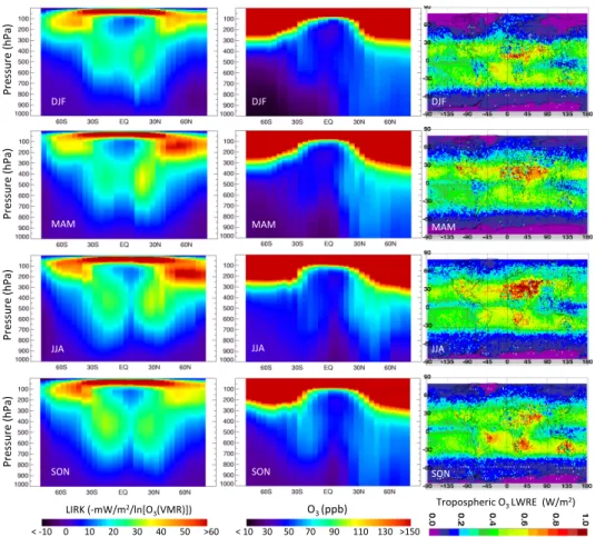
Fig. 1. Logarithmic instantaneous radiative kernels (LIRK) in mWm−2/ln(vmrO3), TES zonal ozone in parts-per-billion (ppb), and longwave radiative effect (LWRE) in Wm−2are shown along across each column respectively. Each row represents data averaged for 2005–2009 for December-January-February (DJF), March-April-May (MAM), June-July-August (JJA), and September-October-November (SON).
profile in volume mixing ratio as a function of altitude z at level l, LTOA is the spectral radiance at frequency ν, zenith
angle φ and azimuth angle θ . The partial derivatives of spec-tral radiance LTOAare provided by the TES operational
ra-diative transfer algorithm, (Clough et al., 2006), and are used within the retrieval algorithm to estimate the vertical distri-butions of trace gases, temperature, water vapor, and clouds (Worden et al., 2004; Bowman et al., 2006). Changes in other atmospheric parameters are incorporated into the LIRK, e.g., retrieved cloud top height will change the altitudes for which
FTOAis sensitive to ozone variations. From Eq. (1), increases
in tropospheric ozone lead to a reduction in OLR consistent with the ozone greenhouse gas effect.
Equation (1) is treated as an operator in a first order Taylor series expansion to calculate the ACCMIP OLR bias from tropospheric ozone as
δOLRj,ml =Hj(zl) [ln qjm(zl) −ln qjobs(zl)] (2)
where qjm(zl)and qjobs(zl)are the model and TES ozone,
re-spectively, at the jt hlocation and the lt haltitude level while
Hj(zl) =
∂FTOAj ∂ln qj(zl)
(3)
is the LIRK at location j and evaluated at altitude zl
dis-cretized at levels l. Consistent with the ozone greenhouse gas effect, the LIRK is negative for increases in tropospheric ozone so that for a positive tropospheric ozone bias between a model and TES at an altitude zl, δOLRj,ml <0. In the
sub-sequent sections, the level l will also refer to corresponding pressure levels.
The total longwave radiative effect (LWRE) is calculated by integrating Eq. (3) in altitude to the tropopause. The LWRE can be thought of as the reduction in OLR to a 100 % change in the tropospheric ozone profile (Worden et al., 2011). Note that the LWRE is a logarithmic change refer-enced to TES ozone and consequently it can not be used to calculate the change to a complete absence of ozone.
TES ozone, LIRK, and LWRE averaged for 2005–2009 are shown in Fig. 1. The LWRE was integrated to the thermal tropopause height derived from the Goddard Modeling and Assimilation Office (GMAO) GEOS-5 (Molod et al., 2012). There is a strong sensitivity in the LIRK of up to 35 m Wm−2
in the mid-troposphere extending as low as 600 hPa and arcing poleward to 200 hPa at 60◦N and 60◦S. The LIRK
increases in the upper troposphere and lower stratosphere with sensitivities well above 60 m Wm−2 per unity change in ln q.The LIRK spatial pattern is remarkably similar to cli-matological relative humidity (RH) distributions, which are at a minimum in subsidence regions especially in the South-ern Hemispheric sub-tropics. Interestingly, low RH in the SH sub-tropics have been linked to equilibrium climate sensitiv-ity (Fasullo and Trenberth, 2012). This similarsensitiv-ity suggests that the LIRK sensitivity is driven primarily by atmospheric opacity which in turn is controlled by a combination of tem-perature, water vapor, and clouds. There is a seasonal migra-tion of the LIRK maximum across the equator, which follows the change in the inter-tropical convergence zone (ITCZ) and is driven primarily by the seasonal shift in cloud distribu-tions.
The seasonal pattern of ozone in the SH is strongly in-fluenced by the presence of biomass burning and lightning leading to a maximum of 60–70 ppb in September-October-November (SON). The impact of biomass burning and light-ning in South America, sub-equatorial Africa, and Indone-sia are clearly seen. Near source regions, the LWRE exceeds 1 Wm−2 during SON. During December-January-February (DJF), ozone from biomass burning in Africa north of the (ITCZ) has similarly high LWRE. In most months, there is a persistently high LWRE (> 1 Wm−2) over the Middle East. This is driven in part by relatively clear skies and a strong thermal contrast that amplifies the ozone greenhouse gas ef-fect. However, in the summer months, there is an ozone en-hancement in the middle troposphere (400–500 hPa) induced by trapping from Saharan and Arabian anticyclones, which also corresponds to the highest magnitude LIRK values in the middle troposphere (Li et al., 2001; Liu et al., 2009).
4 Methodology
4.1 Radiative forcing
Radiative forcing (RF) is a measure of the energy imbalance of the Earth-atmosphere system and is used as a means of quantifying the potential of external agents to perturb that system. In the context of historic climate change, the pertur-bation is referenced from preindustrial (1750s) to the present-day (2000s). In order for the ozone forcing to be taken as a reasonable proxy for the expected temperature response, RF is specifically defined as the change in net irradiance at the tropopause after stratospheric temperatures have re-laxed to radiative-dynamical equilibrium but with the sur-face and atmospheric state held fixed (Forster et al., 1997, 2007). The forcing-response relationship, however, can be more complicated depending on the forcing agent and its distribution (Fels et al., 1980; Hansen et al., 1997, 2007; Shindell and Faluvegi, 2009). Methods of calculating
tropo-spheric ozone RF from models using “off-line” techniques, i.e., radiative transfer calculations performed independently of a climate model’s internal radiation calculation, follow two steps. The first step is to calculate the change in ozone concentrations by forcing a global chemistry-climate model with pre-industrial (usually taken in the 1750s) and present-day concentrations in separate “time-slices”, which is an in-terval of time, e.g., 1750–1760. The second step is to calcu-late the change in longwave and shortwave radiation due to the change in present-day ozone relative to the pre-industrial era using an “off-line” radiative transfer model (RTM) where stratospheric temperatures are allowed to equilibrate result-ing in an adjusted irradiance (Edwards and Slresult-ingo, 1996; Stevenson et al., 2006; Knutti and Hegerl, 2008; Steven-son et al., 2013). Radiative forcing is generally referenced at the tropopause, the definition of which can have a sig-nificant impact on the final calculation, e.g. flat tropopause set at 100, 150 or 200 hPa, zonally invariant and linear with latitude tropopause (Naik et al., 2005; Hansen et al., 2007), chemical tropopause using the 150 ppbv ozone level (Steven-son et al., 2006), and the WMO thermal tropopause (Aghedo et al., 2011b). Radiative forcing is simply the difference be-tween the irradiance at two different time periods, which can be expressed as:
RFm=R(qmp) − R(qmo) (4)
where R is the globally, area-weighted average net irradi-ance (shortwave (SW) plus longwave (LW)) in m Wm−2 in-cluding stratospheric readjustment, qm
p is the vertical
distri-bution (discretized as a vector) of present-day ozone simu-lated by model m, and qm
o is preindustrial ozone for the same
model. Implicit in Eq. (4) is temporal averaging over some time-slice.
4.2 Application to TES data
TES observations directly measure the 9.6 micron ozone band radiances (the primary band where ozone absorbs ther-mal infrared radiation) and have the spectral resolution to disentangle the geophysical quantities, e.g., temperature and clouds, driving ozone band radiative flux variability. These data have the potential to assess model results with respect to the longwave component of ozone radiative forcing. How-ever, differences between satellite and climate model cal-culations need to be considered. TES only measures ther-mal radiance at the top-of-the-atmosphere (TOA). Conse-quently, these measurements do not provide information on the shortwave irradiance. Chemistry-climate models calcu-late the full global and diurnal cycle of ozone whereas TES has a global repeat cycle of 16 days and can only measure twice a day through its ascending and descending nodes. However, Aghedo et al. (2011a) showed that TES sampling is sufficient to capture zonal scale variations in ozone when compared to chemistry-climate model simulations.
The mean ACCMIP bias in OLR from tropospheric ozone is calculated from Eq. (2) as
δOLRjm= 1 Nj X i∈Dj X l∈L
wiHi,l(ln[qmp]i,l−ln[qobsp ]i,l) (5)
where wi are area-weights (to account for the relative areas
of different latitude bands), Djis a set of observed locations, Nj is the number of locations in set Dj, and L is the set
of altitude levels whose maximum value is at the tropopause, which we choose to be the chemical tropopause q = 150 ppb. The domain Djcan be comprised of either grid cells or zonal
bands. In either case, we will define the OLR bias as δOLRjm
where j refers to latitudinal bands or individual grid boxes depending on the context described in the subsequent sec-tions. The global mean OLR bias from tropospheric ozone is calculated by averaging over all Dj and will be denoted as δOLRm. The ACCMIP ensemble mean OLR bias from
tro-pospheric ozone will be denoted as δOLRj for locations Dj
and the ensemble global mean is simply δOLR. Implicit in Eq. (5) is temporal averaging from 2005–2010.
5 Results
5.1 ACCMIP simulations
We use TES observations to evaluate the OLR bias from tropospheric ozone in the chemistry-climate models that participated in ACCMIP. A complete description of the chemistry-climate and chemical transport models along with their short hand designation (CESM-CAM-superfast, CICERO-OsloCTM2, CMAM, GEOSCCM, GFDL-AM3, GISS-E2-R, GISS-E2-TOMAS, HadGEM2,
LMDzOR-INCA, MIROC-CHEM, MOCAGE, NCAR-CAM3.5,
STOC-HadAM3, UM-CAM) can be found in Lamarque et al. (2013). Each were driven by a common set of emis-sions (Lamarque et al., 2010). The experimental design was based on decadal “time-slice” experiments driven by decadal mean sea surface temperatures (SST). The historic periods included 1850, 1980, and 2000 along with 2030 and 2100 time slices that follow the representative concentration pathways (RCP) (van Vuuren et al., 2011). As described by Lamarque et al. (2013) the level of complexity in the chemistry schemes varied significantly between the models. The physical climate was based on prescribed SSTs for most models with the notable exception of the GISS model, which is integrated with a fully coupled ocean-atmosphere model (Shindell et al., 2013). Following Young et al. (2013), model simulations for the 2000 decade were averaged and then interpolated to the domain of the gridded TES product archived along with the ACCMIP simulations at the British Atmospheric Data Archive (BADC), which is composed of 64 pressure levels at 2 × 2.5◦ spatial resolution. These decadal mean model simulations are then compared against TES tropospheric ozone for 2005-2010.
Fig. 2: Zonal bias between ACCMIP models and TES ozone averaged over 2005-2010. Ensemble average of ACCMIP compared to TES ozone is shown under ENS in the bottom right.
25
Fig. 2. Zonal bias between ACCMIP models and TES ozone aver-aged over 2005–2010. Ensemble average of ACCMIP compared to TES ozone is shown under ENS in the bottom right.
5.2 Application to ACCMIP models
We first compare the zonal-vertical difference between the ACCMIP and TES tropospheric ozone from 2005–2010 as shown in Fig. 2 including the ensemble (ENS) in the bottom right. There is a rich diversity in the zonal ozone distribution. In the middle to lower troposphere the agreement is gener-ally within 10–15 ppb. In the Northern Midlatitudes (NMLT), the GISS-E2-R, GISS-E2-TOMAS, and MOCAGE were larger than TES ozone estimates by more than 10 ppb. On the other hand, CICERO-OsloCTM2, HadGEM2, MIROC-CHEM, and CMAM tend to underestimate NMLT ozone rel-ative to TES ozone. In the tropical troposphere, most mod-els tend to underestimate ozone. The upper troposphere and lower stratosphere show stronger differences. The CMAM and MIROC-CHEM models have significantly higher ozone in both the NMLT and the Southern Midlatitudes (SMLT). Conversely, MOCAGE, HadGEM2, STOC-HadAM3, and UM-CAM estimate lower ozone than TES ozone in both the NMLT and SMLT. However, the TES observation operator is
CESM-CAM-superfast 100 1000 CICERO-OsloCTM2 CMAM GEOSCCM 100 1000 GFDL-AM3 GISS-E2-R GISS-E2-R-TOMAS 100 1000 HadGEM2 LMDzORINCA MIROC-CHEM 100 1000 MOCAGE NCAR-CAM 3.5 STOC-HadAM3 100 1000 -80 -50 -25 0 25 50 80 UM-CAM -80 -50 -25 0 25 50 80 ENS -80 -50 -25 0 25 50 80 mWm−2
Fig. 3: Zonal distribution of ACCMIP OLR bias from tropospheric ozone, δOLRj,ml , from 2005-2010. The vertical scale is defined from 1000-100 hPa discretized to TES pressure levels . Color scale is inverted to show that positive δOLRj,ml is a model low ozone bias relative to TES. Ensemble mean bias δOLRjlis denoted by ENS.
26
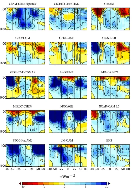
Fig. 3. Zonal distribution of ACCMIP OLR bias from tropospheric ozone, δOLRj,ml , from 2005-2010. The vertical scale is defined from 1000–100 hPa discretized to TES pressure levels. Color scale is inverted to show that positive δOLRj,ml is a model low ozone bias relative to TES. Ensemble mean bias δOLRjl is denoted by ENS.
not applied to these models as Aghedo et al. (2011b), nor is there any bias correction applied to the TES data. Based on ozonesonde comparisons discussed in Sect. 2, TES ozone is systematically high in the Northern Hemisphere, which sug-gests that the high ozone biases in GISS-E2-R and MOCAGE are exacerbated but the slight low ozone bias in the ensemble distribution is likely insignificant. TES upper tropospheric ozone in the tropics is consistent with ozonesonde measure-ments, which indicates that the ensemble model low bias is robust.
The ACCMIP OLR bias from tropospheric ozone,
δOLRj,ml , which is calculated from Eq. (2), is shown in Fig. 3 discretized at TES pressure levels. The zonal cross-section in this figure can be related to the ACCMIP ozone bias in Fig. 2
through Eq. (2). For example, in Fig. 2 a 10 ppb low bias of GISS-E2-R relative to TES ozone at 300 hPa and 15◦S leads to a δOLRj,ml of about 5 m Wm−2 at the same loca-tion as shown in Fig. 3. As quantified by the LIRK in Fig. 1, the thermal contrast between the temperature at which the ozone absorbs in the troposphere and the surface temper-ature along with the low humidity, which decreases atmo-spheric opacity, contributes to the importance of the tropics and subtropics relative to the high latitudes. Consequently, underestimates of tropical and subtropical ozone are ampli-fied in terms of δOLRj,ml relative to the extratropics. Almost half of the ACCMIP models have δOLRj,ml that exceeds 10 m Wm−2at individual pressure levels l. Radiatively sig-nificant differences are not confined to the upper troposphere.
CESM-CAM-superfast CICERO-OsloCTM2 CMAM
GEOSCCM GFDL-AM3 GISS-E2-R
GISS-E2-R-TOMAS HadGEM2 LMDzORINCA
MIROC-CHEM MOCAGE NCAR-CAM 3.5
STOC-HadAM3 UM-CAM ENS
Fig. 4: Spatial distribution of ACCMIP OLR bias from tropospheric ozone, δOLRj
m, from
2005-2010, limited to 80◦S-80◦N, and based on a chemical tropopause q = 150 ppb as diagnosed from
TES. ACCMIP ensemble, δOLRj, is denoted by ENS.
27
mWm-2
Fig. 4. Spatial distribution of ACCMIP OLR bias from tropospheric ozone, δOLRjm, from 2005–2010, limited to 80◦S–80◦N, and based on
a chemical tropopause q = 150 ppb as diagnosed from TES. ACCMIP ensemble, δOLRj, is denoted by ENS.
In several models, tropical differences in ozone at pressures greater than 600 hPa lead to δOLRj,ml >10 m Wm−2.
The ACCMIP OLR bias from tropospheric ozone is the ACCMIP tropospheric ozone bias weighted by the LIRK. Comparing the LIRK distributions in Fig. 1 to the δOLRj,ml in Fig. 3 suggest that in the tropics and SH, δOLRj,ml from models such CESM-superfast, HadGEM-2, MOCAGE, UM-CAM, NCAR-CAM 3.5, STOC-HadAM3 has a strong in-fluence from the LIRK, particularly the positive δOLRj,ml at 500 hPa around 10–15◦S and extending poleward up to 100 hPa around 50◦S. This LIRK spatial pattern is persistent across a number of models in SH as can be seen in the AC-CMIP ensemble mean δOLRjl in Fig. 3. In the NH high lati-tudes, such as with GISS-E2-R at 60◦N and 600 hPa, there is a significant bias in ozone but the attenuated OLR sensitivity makes δOLRj,ml relatively small.
A complimentary perspective is shown in Fig. 4, which shows δOLRjm calculated from Eq. (5) where δOLRj,ml at
each location j is vertically integrated up to the chemical
tropopause of q = 150 ppb diagnosed from TES ozone. Most ACCMIP models have a positive δOLRjm in the SH
trop-ics because they underestimate tropospheric ozone relative to TES tropospheric ozone. The overestimate in the Eastern Tropical Atlantic is a persistent feature in all of the ACCMIP models and is reflected in the ensemble mean. Tropospheric ozone distributions in the tropical Atlantic are driven by a number of processes but are dominated by lightning (Jacob et al., 1996; Jenkins and Ryu, 2004; Sauvage et al., 2007; Bowman et al., 2009). A second persistent feature is the overestimate centered over Southern Africa. Southern equa-torial Africa is an important source of biomass burning (Ed-wards et al., 2006; Aghedo et al., 2007). Satellite-based “top-down” estimates indicate the emissions from biomass burn-ing are significantly underestimated (Arellano et al., 2006; Jones et al., 2009). Local sources of pollution and biomass burning have been associated with upward trends in ozone, particularly in the lower troposphere (Clain et al., 2009). However, the Southern African region has a complex circu-lation pattern that includes both anticyclonic transport and
-50 0 50 100 Latitude -100 0 100 200 300 400 ACCMIP-TES (W/m 2 ) CESM-CAM-superfast CICERO-OsloCTM2 CMAM GEOSCCM GFDL-AM3 GISS-E2-R GISS-E2-TOMAS HadGEM2 LMDzORINCA MIROC-CHEM MOCAGE NCAR-CAM3.5 STOC-HadAM3 UM-CAM ENS A CCM IP -TES (mWm -2) Latitude
Fig. 5: Zonal δOLRj
mbetween ACCMIP and TES from 2005-2010, limited to 80◦S-80◦N, and is
based on a TES diagnosed chemical tropopause (q = 150 ppb). The “ENS” refers to the ACCMIP ensemble average, δOLRj. Positive values indicate model ozone is biased low relative to TES ozone
and consequently the model OLR is biased high relative to TES OLR.
28
Fig. 5. Zonal δOLRjmbetween ACCMIP and TES from 2005-2010,
limited to 80◦S–80◦N, and is based on a TES diagnosed chem-ical tropopause (q = 150 ppb). The “ENS” refers to the ACCMIP ensemble average, δOLRj. Positive values indicate model ozone is
biased low relative to TES ozone and consequently the model OLR is biased high relative to TES OLR.
recirculation as well as direct eastward and westward trans-port (Garstang et al., 1996; Sinha et al., 2004). Upwind sources of ozone precursors from biomass burning, pollu-tion, and lightning can be advected across Southern Africa and out to the remote Pacific (Chatfield and Delany, 1990; Chatfield et al., 2002). Some of the radiatively strongest dif-ferences (>200 mW/m2) in δOLRjm, e.g, GISS-E2-R and
NCAR-CAM3.5, are throughout the tropical Pacific, which may contribute to the positive SH δOLRj. The ACCMIP
ensemble shows a persistent pattern in the tropical Pacific with a local maximum near 75 m Wm−2. Comparison of the tropical distribution in Fig. 4 with the zonal-vertical distribu-tion in Fig. 3 of δOLRjm, points to the combination of low
ozone throughout the troposphere that is amplified by the strong mid-tropospheric radiative sensitivity of the southern branch of the LIRK in Fig. 1. Tropical ozone is sensitive to convective mass flux, height, and subsidence, particularly in the Eastern Pacific (Liu et al., 2010). These factors in con-junction with ozone precursor uncertainties could help ex-plain these features, though they are more prevalent during El Ni˜no periods such as in 2006 (Nassar et al., 2009; Chan-dra et al., 2009) which are not well simulated in ACCMIP due to decadally averaged SST boundary conditions.
The SH tropics and subtropics dominate radiative dif-ferences as shown by the vertically integrated zonal dis-tribution in Fig. 5. The ensemble mean δOLRj is high
by about 120 m Wm−2 between 10–20◦S. The mean bias is strongly influenced by MOCAGE, CESM-CAM, and NCAR-CAM3.5, whose δOLRjm varies from 200–
400 m Wm−2 though the latter two are driven by similar physical climate models. In the NH extratropics, the
en-CESM-CAM-superfast CICERO-OsloCTM2 CMAM GEOSCCM GFDL-AM3 GISS-E2-R GISS-E2-TOMAS HadGEM2 LMDzORINCA MIROC-CHEM MOCAGE NCAR-CAM3.5 STOC-HadAM3 UM-CAM 0 50 100 150 250 300 350 400 450 500 ∆OLR HmWm-2L ACCMIP RF HmWm -2 L
Fig. 6. ACCMIP ozone radiative forcing from preindustrial to present day as a function of δOLRm, which is the difference
be-tween ACCMIP model ozone and TES ozone weighted by the TES Instantaneous Radiative Kernel. The δOLR is integrated through the TES diagnosed chemical tropopause q = 150 ppb and averaged from 2005–2010.
semble mean δOLRj ≈0 mWm−2 with the extrema near
100 m Wm−2 at 30◦N decreasing poleward at a rate be-tween linear and exponential. Systematic overestimates in the northern high latitudes in the TES ozone data will not strongly effect the ensemble mean bias because of the lower OLR sensitivity to tropospheric ozone. On the other hand, the SH low bias is robust because of the small upper tropospheric system errors in the TES retrieval.
5.3 Implications for ACCMIP ozone radiative forcing
We explore whether present-day OLR model bias from tro-pospheric ozone is correlated with model ozone RF and whether this relationship can be used to reduce our uncer-tainty in preindustrial to present day ozone RF. The cause of ACCMIP OLR bias from tropospheric ozone is a complex combination of uncertainties related to both the physical and chemical climate. Some of these differences are related to natural background conditions, e.g., lightning NOx. Model
biases for present-day background ozone may be expected to be correlated with respective biases from pre-industrial back-ground ozone. Young et al. (2013) showed, for example, that ACCMIP models with high ozone burdens over the present-day had high burdens for the other periods of time including the preindustrial period. Uncertainties in present day emis-sions and their chemical transformation could result in sig-nificant biases in tropospheric ozone. Consequently, present day measurements have the potential to inform preindustrial to present day ozone radiative forcing.
In Table 1, the domain Dj of δOLRjm in Eq. (5) is
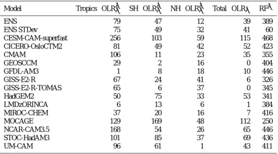
de-fined for the tropics (15◦S–15◦N), NH and SH extra-tropics. Tropical biases contributed the most to the global δOLRm
with some zonal δOLRjm>250 m Wm−2. There are 5 of
the 15 models with tropical δOLRim>100 m Wm−2. While most of the models underestimate ozone in the tropics–and hence have a positive δOLRjm, there are 2 models that have
Table 1. ACCMIP OLR bias from tropospheric ozone (δOLRjm) and ozone radiative forcing (RFm) in m Wm−2. The ozone RFmis taken
from (Stevenson et al., 2013) and is defined relative to 1750 and at a climatological thermal tropopause. The ACCMIP ensemble mean and 1-σ are shown in the last column of the first two rows. Tropics are defined from 15◦S–15◦N.
Model Tropics δOLRjm SH δOLRjm NH δOLRjm Total δOLRm RFm
ENS 79 47 12 39 389 ENS STDev 75 49 32 41 60 CESM-CAM-superfast 256 103 59 115 468 CICERO-OsloCTM2 81 49 42 52 423 CMAM 106 11 23 35 355 GEOSCCM 29 2 −16 0 404 GFDL-AM3 1 −8 −18 −10 446 GISS-E2-R 67 24 −41 6 326 GISS-E2-R-TOMAS 65 6 −37 0 345 HadGEM2 50 75 33 53 341 LMDzORINCA −6 13 −6 1 384 MIROC-CHEM −37 20 16 7 416 MOCAGE 129 169 48 112 250 NCAR-CAM3.5 168 54 26 65 446 STOC-HadAM3 101 85 37 69 436 UM-CAM 96 61 −1 43 411 Slope=0.60 @0.29, 0.91D, R2=0.59 0 20 40 60 80 100 120 0 20 40 60 80 100 120 È∆OLRmÈ HmWm-2L Dm HmWm -2L
Fig. 7. The deviation of ACCMIP ozone radiative forcing from an ensemble mean versus |δOLRm|, which is the magnitude of the
difference between model ozone and TES ozone weighted by the TES Instantaneous Radiative Kernel. The mean is calculate from an subset of models whose |δOLRm|<10 m Wm−2. The δOLR
is integrated through the TES diagnosed chemical tropopause q = 150 ppb and averaged from 2005-2010. The correspondence be-tween the colors and models is the same as in Fig. 6. The brackets for the slope represent the uncertainty at the 95 % confidence.
a negative δOLRjm. Similarly, the SH δOLRjm reaches as
much as 170 m Wm−2. The NH has a much wider response with about half of the models having a δOLRjm as high as
60 m Wm−2. There are 5 models whose total δOLRmare less
than 10 m Wm−2whereas most are greater than 30 m Wm−2. The ensemble mean and standard deviation for δOLRm is δOLR = 39 ± 41 m Wm−2, which reflects this variability.
In order to explore the implications of these biases on ozone radiative forcing, the global δOLRm is
com-pared to ACCMIP ozone RF in Fig. 6. The ACCMIP
ozone RF is based on the climatological thermal tropopause and the ozone RF has been extended from 1850 to 1750 by adding 40 m Wm−2 (Skeie et al., 2011; Steven-son et al., 2013). There is a wide range of ozone RF estimates from 210-428 m Wm−2 with a mean of 384 ± 60 m Wm−2. To investigate whether there is a re-lationship between model ozone RF and the magnitude of δOLRm we first choose a subset of models whose |δOLRm|<10 m Wm−2
(GEOSCCM,GISS-E2R,GISS-E2-R-TOMAS,LMDzORINCA,MIROC-CHEM). The ozone RF mean and standard deviation of this subset is 375 ± 38.4 m Wm−2. We then calculate the ozone RF abso-lute deviation of all the ACCMIP models with respect to the subset mean as
4m= R¯s−Rm
(6)
where ¯Rsis the subset ACCMIP ensemble mean ozone RF. The ACCMIP deviation is shown as a function of |δOLRm|
in Fig. 7. The color scheme in Fig. 7 is the same as in Fig. 6. The slope of the linear fit shown in Fig. 7 is 0.60 with a 95 % confidence interval of [0.29, 0.91] and R2=
0.59. This correlation is largely driven by two models whose
|δOLRm|>100 m Wm−2. If these models are not included
then R2=0.18 and the null hypothesis, i.e., there is no sig-nificant relationship between ACCMIP OLR bias and ozone RF, can only be rejected at the 80 % confidence level. It’s interesting to note that these two models – CESM-CAM and MOCAGE – have the highest (538) and lowest (309), respec-tively, ozone radiative forcing. The ozone RF is driven in part by a change of only 4.8 Dobson Units (DU) in ozone for MOCAGE but a 10 DU ozone change for CESM-CAM from
preindustrial to present-day (Stevenson et al., 2013; Young et al., 2013).
The difference in correlation between the ACCMIP en-semble subgroups provides a reasonable basis for enen-semble selection. As a limitation for ensemble selection, TES obser-vations can not be used to distinguish between models for which there is no correlation between model OLR bias from tropospheric ozone and model ozone RF. Therefore, models are selected for which |δOLRm|<100 m Wm−2 and
there-fore 4m<86 m Wm−2. The ACCMIP radiative forcing
un-der these conditions is 394 ±42 m Wm−2. The mean is about the same and the standard deviation has been reduced by 28 % relative to 389± 60 m Wm−2, which is the ACCMIP ensemble mean ozone RF in Table 1. While this estimate has reduced variability relative to the full ACCMIP ensem-ble ozone radiative forcing, it does not fully account for other sources of uncertainty, e.g., differences in radiative transfer models (Forster et al., 2011).
6 Conclusions
We have presented an evaluation of ACCMIP OLR from tro-pospheric ozone using TES ozone and LIRK data. We fur-ther explored the implication of this evaluation on ozone RF estimates. We find a significant correlation R2=0.59 between |δOLRm|and the absolute deviation from the
AC-CMIP ensemble ozone RF, 4m. However, this correlation
drops to R2=0.18 if we only include models for which
|δOLR| < 100 m Wm−2. Using this change in correlation as a basis for ensemble selection, we estimate the ACCMIP RF to be 394±42 m Wm−2(1 standard deviation), which is close to the ACCMIP full ensemble mean RF of Stevenson et al. (2013) but with about 30 % less standard deviation. We note that our calculation used only 14 of the 16 models used by Stevenson et al. (2013). This result is in contrast to the lack of correlation across the full ACCMIP ensemble between present day tropospheric ozone bias and the change in ozone burden from preindustrial to present day reported by Young et al. (2013). However, our estimate does not account for bias associated with preindustrial emissions nor with others sources of uncertainty such as differences in the physical cli-mate or radiative transfer algorithms. The results further sug-gest that any causal relationship between present day model OLR bias and model ozone RF could be model specific and not necessarily reflective of any general relationship between present day OLR and ozone RF.
We investigated the spatial patterns driving present-day bias in ACCMIP OLR from tropospheric ozone. These pat-terns were driven in the ACCMIP models by variations in the SH tropics and sub-tropics where the ensemble mean
δOLRj reached 100 m Wm−2 in some regions. Persistent
patterns of δOLRjmwere centered over the tropical Atlantic
and over Southern Africa. While the importance of upper tro-pospheric ozone to ozone RF is known (Lacis et al., 1990;
Gauss et al., 2003), significant δOLRj,ml (> 10 m Wm−2) could be attributed to ACCMIP ozone bias at pressures ex-ceeding 600 hPa. While the modest low bias in δOLRjm in
the NH can be attributed in part to a systematic TES retrieval overestimate, the ACCMIP SH low bias in δOLRjmis robust
in light of the smaller TES tropical retrieval systematic er-rors.
Our results demonstrate a motivation for developing more sophisticated approaches that incorporate explicit statistical modeling of present day OLR bias from tropospheric ozone and ozone RF. Such approaches would permit a more rigor-ous means of weighting model ozone RF based upon their relationship to observations (Tebaldi et al., 2005; Berliner and Kim, 2008). There is considerable interest in using both data and an ensemble of climate models to understand his-toric change and probabilistically weight future projections (Knutti et al., 2002; Collins, 2007; Tebaldi and Knutti, 2007). There has been little to no application of these methodologies to chemistry-climate projections or the attribution of historic climate change to chemically active agents as has been done in detection and attribution studies for temperature (Hegerl et al., 1996; Santer et al., 2007; Huber and Knutti, 2012). There is also the potential of using advanced data assimi-lation techniques to attribute observed OLR to natural and anthropogenic emissions at finer spatial resolution (Bowman and Henze, 2012). The combination of these approaches with a process-based analysis (Eyring et al., 2005, 2006; Waugh and Eyring, 2008) can help test radiatively important pro-cesses against observations in a manner that can reduce our uncertainty in ozone RF and increase the reliability of future projections.
Acknowledgements. We thank the anonymous reviewers for their thoughtful comments and suggestions. The manuscript is greatly improved as a consequence.
This research was carried out at the Jet Propulsion Laboratory, Cal-ifornia Institute of Technology, under a contract with NASA. The TES monthly ozone and IRK dataset was developed using tech-niques from the obs4MIP activity (http://obs4mips.llnl.gov:8080/ wiki/)
The National Center for Atmospheric Research (NCAR) is spon-sored by the National Science Foundation.
KB and HW acknowledges the support of the NASA Aura ROSES program. KB also acknowledges some useful codes from Adetutu Aghedo and Rachel Hodos in the initial processing of TES data to netcdf files.
ACCMIP is organized under the auspices of Atmospheric Chem-istry and Climate (AC&C), a project of International Global At-mospheric Chemistry (IGAC) and Stratospheric Processes And their Role in Climate (SPARC) under the International Geosphere-Biosphere Project (IGBP) and World Climate Research Program (WCRP).
The CESM project is supported by the National Science Foundation and the Office of Science (BER) of the US Department of Energy.
The National Center for Atmospheric Research is operated by the University Corporation for Atmospheric Research under sponsor-ship of the National Science Foundation.
GZ acknowledges NIWA HPCF facility and funding from New Zealand Ministry of Science and Innovation.
The work of DB and PC was funded by the US Dept. of En-ergy (BER), performed under the auspices of LLNL under Contract DE-AC52-07NA27344, and used the supercomputing resources of NERSC under contract No. DE-AC02-05CH11231.
Ghan was supported by the US Department of Energy Office of Sci-ence Decadal and Regional Climate Prediction using Earth System Models (EaSM) program. The Pacific Northwest National Labora-tory (PNNL) is operated for the DOE by Battelle Memorial Institute under contract DE-AC06-76RLO 1830.
W. J. Collins, G. A. Folberth, F. O’Connor and S. T. Rumbold were supported by the Joint DECC and Defra Integrated Climate Pro-gramme (GA01101).
VN and LWH acknowledge efforts of GFDL’s Global Atmospheric Model Development Team in the development of the GFDL-AM3 and Modeling Services Group for assistance with data processing The GEOSCCM work was supported by the NASA Modeling, Analysis and Prediction program, with computing resources pro-vided by NASA’s High-End Computing Program through the NASA Advanced Supercomputing Division.
The MIROC-CHEM calculations were performed on the NIES su-percomputer system (NEC SX-8R), and supported by the Environ-ment Research and Technology DevelopEnviron-ment Fund (S-7)of the Min-istry of the Environment, Japan.
The STOC-HadAM3 work was supported by cross UK research council grant NE/I008063/1 and used facilities provided by the UK’s national high-performance computing service, HECToR, through Computational Modelling Services (CMS), part of the NERC National Centre for Atmospheric Science (NCAS). The LMDz-OR-INCA simulations were done using computing ressources provided by the CCRT/GENCI computer center of the CEA.
The CICERO-OsloCTM2 simulations were done within the projects SLAC (Short Lived Atmospheric Components) and EarthClim funded by the Norwegian Research Council.
The MOCAGE simulations were supported by M´et´eo-France and CNRS. Supercomputing time was provided by M´et´eo-France/DSI supercomputing center.
DS and Y. H. Lee acknowledges support from the NASA MAP and ACMAP programs.
DP would like to thank the Canadian Foundation for Climate and Atmospheric Sciences for their long-running support of CMAM development.
Edited by: M. Dameris
References
Aghedo, A. M., Schultz, M. G., and Rast, S.: The influence of African air pollution on regional and global tropospheric ozone, Atmos. Chem. Phys., 7, 1193–1212, doi:10.5194/acp-7-1193-2007, 2007.
Aghedo, A. M., Bowman, K. W., Shindell, D. T., and Faluvegi, G.: The impact of orbital sampling, monthly averaging and vertical resolution on climate chemistry model evaluation with satellite observations, Atmos. Chem. Phys., 11, 6493–6514, doi:10.5194/acp-11-6493-2011, 2011a.
Aghedo, A. M., Bowman, K. W., Worden, H. M., Kulawik, S. S., Shindell, D. T., Lamarque, J. F., Faluvegi, G., Parring-ton, M., Jones, D. B. A., and Rast, S.: The vertical distri-bution of ozone instantaneous radiative forcing from satellite and chemistry climate models, J. Geophys. Res., 116, D01305, doi:10.1029/2010JD014243, 2011b.
Arellano, A. F., Kasibhatla, P. S., Giglio, L., van der Werf, G. R., Randerson, J. T., and Collatz, G. J.: Time-dependent inversion es-timates of global biomass-burning CO emissions using Measure-ment of Pollution in the Troposphere (MOPITT) measureMeasure-ments, J. Geophys. Res., 111, D09303, doi:10.1029/2005JD006613, 2006.
Beer, R.: TES on the Aura Mission: Scientific Objectives, Mea-surements, and Analysis Overview, IEEE Trans. Geosci. Remote Sens., 44, 1102–1105, 2006.
Berliner, L. M. and Kim, Y.: Bayesian Design and Analysis for Superensemble-Based Climate Forecasting, J. Climate, 21, 1891–1910, 2008.
Bowman, K. and Henze, D. K.: Attribution of direct ozone radiative forcing to spatially resolved emissions, Geophys. Res. Lett., 39, L22704, doi:10.1029/2012GL053274, 2012.
Bowman, K., Worden, J., Steck, T., Worden, H., Clough, S., and Rodgers, C.: Capturing time and vertical variability of tropo-spheric ozone: A study using TES nadir retrievals, J. Geophys. Res., 107, 4723, doi:10.1029/2002JD002150, 2002.
Bowman, K. W., Rodgers, C. D., Kulawik, S. S., Worden, J., Sarkissian, E., Osterman, G., Steck, T., Lou, M., Elder-ing, A., Shephard, M., Worden, H., Lampel, M., Clough, S., Brown, P., Rinsland, C., Gunson, M., and Beer, R.: Tropo-spheric Emission Spectrometer: Retrieval Method and Error Analysis, IEEE Trans. Geosci. Remote Sens., 44, 1297–1307, doi:10.1109/TGRS.2006.871234, 2006.
Bowman, K. W., Jones, D. B. A., Logan, J. A., Worden, H., Boersma, F., Chang, R., Kulawik, S., Osterman, G., Hamer, P., and Worden, J.: The zonal structure of tropical O3and CO as
observed by the Tropospheric Emission Spectrometer in Novem-ber 2004 Part 2: Impact of surface emissions on O3and its
pre-cursors, Atmos. Chem. Phys., 9, 3563–3582, doi:10.5194/acp-9-3563-2009, 2009.
Boxe, C. S., Worden, J. R., Bowman, K. W., Kulawik, S. S., Neu, J. L., Ford, W. C., Osterman, G. B., Herman, R. L., Eldering, A., Tarasick, D. W., Thompson, A. M., Doughty, D. C., Hoff-mann, M. R., and Oltmans, S. J.: Validation of northern latitude Tropospheric Emission Spectrometer stare ozone profiles with ARC-IONS sondes during ARCTAS: sensitivity, bias and error analysis, Atmos. Chem. Phys., 10, 9901–9914, doi:10.5194/acp-10-9901-2010, 2010.
Chandra, S., Ziemke, J. R., Duncan, B. N., Diehl, T. L., Livesey, N. J., and Froidevaux, L.: Effects of the 2006 El Ni˜no on
tro-pospheric ozone and carbon monoxide: implications for dynam-ics and biomass burning, Atmos. Chem. Phys., 9, 4239–4249, doi:10.5194/acp-9-4239-2009, 2009.
Chatfield, R. B. and Delany, A.: Convection links biomass burning to increased tropical ozone: However, models will tend to over-predict O3, J. Geophys. Res.-Atmos., 95, 18473–18488, 1990.
Chatfield, R. B., Guo, Z., Sachse, G. W., Blake, D. R., and Blake, N. J.: The subtropical global plume in the Pacific Exploratory Mission-Tropics A (PEM-Tropics A), PEM-Tropics B, and the Global Atmospheric Sampling Program (GASP): How tropical emissions affect the remote Pacific, J. Geophys. Res., 107, 4278, doi:10.1029/2001JD000497, 2002.
Clain, G., Baray, J. L., Delmas, R., Diab, R., Leclair de Bellevue, J., Keckhut, P., Posny, F., Metzger, J. M., and Cammas, J. P.: Tro-pospheric ozone climatology at two Southern Hemisphere trop-ical/subtropical sites, (Reunion Island and Irene, South Africa) from ozonesondes, LIDAR, and in situ aircraft measurements, Atmos. Chem. Phys., 9, 1723–1734, doi:10.5194/acp-9-1723-2009, 2009.
Clough, S. and Iacono, M.: Line-by-line Calculation of atmospheric fluxes and cooling rates.2. application to carbon-dioxide, ozone, methane, nitrous-oxide and the halocarbons, J. Geophys. Res.-Atmos., 100, 16519–16535, 1995.
Clough, S., Shepard, M., Worden, J. R., Brown, P. D., Worden, H. M., Lou, M., Rodgers, C., Rinsland, C., Goldman, A., Brown, L., Eldering, A., Kulawik, S. S., Cady-Pereira, K., Osterman, G., and Beer, R.: Forward Model and Jacobians for Tropospheric Emission Spectrometer Retrievals, IEEE Trans. Geosci. Remote Sens., 44, 1308–1323, 2006.
Collins, M.: Ensembles and probabilities: a new era in the predic-tion of climate change, Phil. Trans. R. Soc. A, 365, 1957–1970, doi:10.1098/rsta.2007.2068, 2007.
Collins, W. J., Sitch, S., and Boucher, O.: How vegetation impacts affect climate metrics for ozone precursors, J. Geophys. Res., 115, doi:10.1029/2010JD014187, 2010.
Connor, T. C., Shephard, M. W., Payne, V. H., Cady-Pereira, K. E., Kulawik, S. S., Luo, M., Osterman, G., and Lampel, M.: Long-term stability of TES satellite radiance measurements, At-mos. Meas. Tech., 4, 1481–1490, doi:10.5194/amt-4-1481-2011, 2011.
Edwards, D. P., Emmons, L. K., Gille, J. C., Chu, A., Atti´e, J.-L., Giglio, L., Wood, S. W., Haywood, J., Deeter, M. N., Massie, S. T., Ziskin, D. C., and Drummond, J. R.: Satellite-observed pol-lution from Southern Hemisphere biomass burning, J. Geophys. Res.-Atmos., D14312, doi:10.1029/2005JD006655, 2006. Edwards, J. M. and Slingo, A.: Studies with a flexible new
radiation code. I: Choosing a configuration for a large-scale model, Q. J. Roy. Meteorol. Soc., 122, 689–719, doi:10.1002/qj.49712253107, 1996.
Eldering, A., Kulawik, S. S., Worden, J., Bowman, K., and Os-terman, G.: Implementation of cloud retrievals for TES atmo-spheric retrievals: 2. Characterization of cloud top pressure and effective optical depth retrievals, J. Geophys. Res., 113, D16S37, doi:10.1029/2007JD008858, 2008.
Eyring, V., Harris, N., Rex, M., Sheperd, T., Fahey, D., Amanatidis, G., Austin, J., Chipperfield, M., Dameris, M., De, P., Forster, F., Gettelman, A., Graf, H., Nagashima, T., Newman, P., Pawson, S., Prather, M. J., Pyle, J. A., Salawitch, J., Santer, B., and Waugh, D. W.: A Strategy for Process-Oriented Validation of Coupled
Chemistry–Climate Models, B. Am. Meteorol. Soc., 86, 1117– 1133, doi:10.1175/BAMS-86-8-1117, 2005.
Eyring, V., Butchart, N., Waugh, D. W., Akiyoshi, H., Austin, J., Bekki, S., Bodeker, G. E., Boville, B. A., Br¨uhl, C., Chipper-field, M. P., Cordero, E., Dameris, M., Deushi, M., Fioletov, V. E., Frith, S. M., Garcia, R. R., Gettelman, A., Giorgetta, M. A., Grewe, V., Jourdain, L., Kinnison, D. E., Mancini, E., Manzini, E., Marchand, M., Marsh, D. R., Nagashima, T., Newman, P. A., Nielsen, J. E., Pawson, S., Pitari, G., Plummer, D. A., Rozanov, E., Schraner, M., Shepherd, T. G., Shibata, K., Stolarski, R. S., Struthers, H., Tian, W., and Yoshiki, M.: Assessment of tem-perature, trace species, and ozone in chemistry-climate model simulations of the recent past, J. Geophys. Res., 111, D22308, doi:10.1029/2006JD007327, 2006.
Fasullo, J. T. and Trenberth, K. E.: A Less Cloudy Future: The Role of Subtropical Subsidence in Climate Sensitivity, Science, 338, 792–794, 2012.
Fels, S. B., Mahlman, J. D., Schwarzkopf, M. D., and Sinclair, R. W.: Stratospheric Sensitivity to Perturbations in Ozone and Carbon Dioxide: Radiative and Dynamical Response, Journal of the Atmospheric Sciences, 37, 2265–2297, doi:10.1175/1520-0469(1980)037<2265:SSTPIO>2.0.CO;2, 1980.
Forster, P., Ramaswamy, V., Artaxo, P., Berntsen, T., Betts, R., Fa-hey, D., Haywood, J., Lean, J., Lowe, D., Myhre, G., Nganga, J., Prinn, R., Raga, G., Schulz, M., and Dorland, R. V.: Cli-mate Change 2007: The Physical Science Basis. Contribution of Working Group I to the Fourth Assessment Report of the Inter-governmental Panel on Climate Change, chap. Changes in Atmo-spheric Constituents and in Radiative Forcing, 131–217, Cam-bridge University Press, 2007.
Forster, P. M., Fomichev, V. I., Rozanov, E., Cagnazzo, C., Jonsson, A. I., Langematz, U., Fomin, B., Iacono, M. J., Mayer, B., Mlawer, E., Myhre, G., Portmann, R. W., Akiyoshi, H., Falaleeva, V., Gillett, N., Karpechko, A., Li, J., Lemen-nais, P., Morgenstern, O., Oberl¨ander, S., Sigmond, M., and Shibata, K.: Evaluation of radiation scheme performance within chemistry climate models, J. Geophys. Res., 116, doi:10.1029/2010JD015361, , 2011.
Forster, P. M. F., Freckleton, R. S., and Shine, K. P.: On aspects of the concept of radiative forcing, Clim. Dynam., 13, 547–560, doi:10.1007/s003820050182, 1997.
Garstang, M., Tyson, P. D., Swap, R., Edwards, M., Kallberg, P., and Lindesay, J. A.: Horizontal and vertical transport of air over southern Africa, J. Geophys. Res.-Atmos., 101, 23721–23736, 1996.
Gauss, M., Myhre, G., Pitari, G., Prather, M. J., Isaksen, I. S. A., Berntsen, T. K., Brasseur, G. P., Dentener, F. J., Derwent, R. G., Hauglustaine, D. A., Horowitz, L. W., Jacob, D. J., Johnson, M., Law, K. S., Mickley, L. J., Muller, J.-F., Plantevin, P.-H., Pyle, J. A., Rogers, H. L., Stevenson, D. S., Sundet, J. K., van Weele, M., and Wild, O.: Radiative forcing in the 21st century due to ozone changes in the troposphere and the lower stratosphere, J. Geophys. Res., 108, 4292, doi:10.1029/2002JD002624, 2003. Hansen, J., Sato, M., and Ruedy, R.: Radiative Forcing and climate
response, J. Geophys. Res., 102, 6831–6864, 1997.
Hansen, J., Sato, M., Kharecha, P., Russell, G., Lea, D. W., and Siddal, M.: Climate change and trace gases, Phil. Trans. R. Soc. A, 365, 1925–1954, doi:10.1098/rsta.2007.2052, 2007.
Hegerl, G. C., von Storch, H., Hasselmann, K., Santer, B. D., Cubasch, U., and Jones, P. D.: Detecting Greenhouse-Gas-Induced Climate Change with an Optimal Fingerprint Method, J. Climate, 9, 2281–2306, 1996.
Huber, M. and Knutti, R.: Anthropogenic and natural warming in-ferred from changes in Earth’s energy balance, Nature Geosci, 5, 31–36, doi:10.1038/ngeo1327, 2012.
Jacob, D., Heikes, B. G., Fan, S.-M., Logan, J. A., Mauzerall, D. L., Bradshaw, J. D., Singh, H. B., Gregory, G. L., Talbot, R. W., Blake, D. R., and Sachse, G. W.: Origin of ozone and NOxin the
tropical troposphere: A photochemical analysis of aircraft obser-vations over the South Atlantic basin, J. Geophys. Res.-Atmos., 101, 24235–24250, doi:10.1029/96JD00336, 1996.
Jenkins, G. S. and Ryu, J.-H.: Linking horizontal and vertical trans-ports of biomass fire emissionsto the tropical Atlantic ozone paradox during the Northern Hemisphere winter season: clima-tology, Atmos. Chem. Phys., 4, 449–469, doi:10.5194/acp-4-449-2004, 2004.
Jones, D. B. A., Bowman, K. W., Logan, J. A., Heald, C. L., Liu, J., Luo, M., Worden, J., and Drummond, J.: The zonal struc-ture of tropical O3 and CO as observed by the Tropospheric
Emission Spectrometer in November 2004 –Part 1: Inverse mod-eling of CO emissions, Atmos. Chem. Phys., 9, 3547–3562, doi:10.5194/acp-9-3547-2009, 2009.
Knutti, R. and Hegerl, G. C.: The equilibrium sensitivity of the Earth’s temperature to radiation changes, Nature Geosci., 1, 735– 743, 2008.
Knutti, R., Stocker, T. F., Joos, F., and Plattner, G.-K.: Constraints on radiative forcing and future climate change from observations and climate model ensembles, Nature, 416, 719–722, 2002. Kulawik, S. S., Worden, J., Eldering, A., Bowman, K., Gunson, M.,
Osterman, G. B., Zhang, L., Clough, S. A., Shephard, M. W., and Beer, R.: Implementation of cloud retrievals for Tropospheric Emission Spectrometer (TES) atmospheric retrievals: part 1. De-scription and characterization of errors on trace gas retrievals, J. Geophys. Res., 111, D24204, doi:10.1029/2005JD006733, 2006. Lacis, A. A., Wuebbles, D. J., and Logan, J. A.: Radiative Forcing of Climate by Changes in the Vertical Distribution of Ozone, J. Geophys. Res., 95, 9971–9981, doi:10.1029/JD095iD07p09971, 1990.
Lamarque, J.-F., Bond, T. C., Eyring, V., Granier, C., Heil, A., Klimont, Z., Lee, D., Liousse, C., Mieville, A., Owen, B., Schultz, M. G., Shindell, D., Smith, S. J., Stehfest, E., Van Aar-denne, J., Cooper, O. R., Kainuma, M., Mahowald, N., Mc-Connell, J. R., Naik, V., Riahi, K., and van Vuuren, D. P.: His-torical (1850–2000) gridded anthropogenic and biomass burning emissions of reactive gases and aerosols: methodology and ap-plication, Atmos. Chem. Phys., 10, 7017–7039, doi:10.5194/acp-10-7017-2010, 2010.
Lamarque, J. F., Shindell, D. T., Josse, B., Young, P. J., Cionni, I., Eyring, V., Bergmann, D., Cameron-Smith, P., Collins, W. J., Do-herty, R., Dalsoren, S., Faluvegi, G., Folberth, G., Ghan, S. J., Horowitz, L. W., Lee, Y. H., MacKenzie, I. A., Nagashima, T., Naik, V., Plummer, D., Righi, M., Rumbold, S. T., Schulz, M., Skeie, R. B., Stevenson, D. S., Strode, S., Sudo, K., Szopa, S., Voulgarakis, A., and Zeng, G.: The Atmospheric Chemistry and Climate Model Intercomparison Project (ACCMIP): overview and description of models, simulations and climate diagnostics, Geosci. Model Dev., 6, 179–206, doi:10.5194/gmd-6-179-2013,
2013.
Levy, II., H., Schwarzkopf, M. D., Horowitz, L., Ramaswamy, V., and Findell, K. L.: Strong sensitivity of late 21st century climate to projected changes in short-lived air pollutants, J. Geophys. Res., 113, D06102, doi:10.1029/2007JD009176, 2008.
Li, Q., Jacob, D. J., Logan, J. A., Bey, I., Yantosca, R. M., Liu, H., Martin, R. V., Fiore, A. M., Field, B. D., Dun-can, B. N., and Thouret, V.: A tropospheric ozone maximum over the Middle East, Geophys. Res. Lett., 28, 3235–3238, doi:10.1029/2001GL013134, 2001.
Liu, J., Logan, J., Jones, D. B. A., Livesey, N. J., Megretskaia, I., Carouge, C., and Nedelec, P.: Analysis of CO in the tropi-cal troposphere using Aura satellite data and the GEOS-Chem model: insights into transport characteristics of the GEOS me-teorological products, Atmos. Chem. Phys., 10, 12207–12232, doi:10.5194/acp-10-12207-2010, 2010.
Liu, J. J., Jones, D. B. A., Worden, J. R., Noone, D., Parrington, M., and Kar, J.: Analysis of the summertime buildup of tropospheric ozone abundances over the Middle East and North Africa as ob-served by the Tropospheric Emission Spectrometer instrument, J. Geophys. Res., 114, D05304, doi:10.1029/2008JD010993, 2009. Molod, A., Takacs, L., Suarez, M., Bacmeister, J., Song, I., and Eichmann, A.: The GEOS-5 Atmospheric General Circulation Model: Mean Climate and Development from MERRA to For-tuna, Tech. Rep. 28, Goddard Space Flight Center, 2012. Naik, V., Mauzerall, D., Horowitz, L., Schwarzkopf, M. D.,
Ramaswamy, V., and Oppenheimer, M.: Net radiative forc-ing due to changes in regional emissions of tropospheric ozone precursors, J. Geophys. Res.-Atmos., 110, D24306, doi:10.1029/2005JD005908, 2005.
Nassar, R., Logan, J., Worden, H., Megretskaia, I. A., Bowman, K., Osterman, G., Thompson, A. M., Tarasick, D. W., Austin, S., Claude, H., Dubey, M. K., Hocking, W. K., Johnson, B. J., Joseph, E., Merrill, J., Morris, G. A., Newchurch, M., Olt-mans, S. J., Posny, F., and Schmidlin, F.: Validation of Tropo-spheric Emission Spectrometer (TES) Nadir Ozone Profiles Us-ing Ozonesonde Measurements, J. Geophys. Res, 113, D15S17, doi:10.1029/2007JD008819, 2008.
Nassar, R., Logan, J. A., Megretskaia, I. A., Murray, L. T., Zhang, L., and Jones, D. B. A.: Analysis of tropical tropospheric ozone, carbon monoxide, and water vapor during the 2006 El Ni˜no using TES observations and the GEOS-Chem model, J. Geophys. Res., 114, D17304, doi:10.1029/2009JD011760, 2009.
Osterman, G., Kulawik, S., Worden, H., Richards, N., Fisher, B., Eldering, A., Shephard, M., Froidevaux, L., Labow, G., Luo, M., Herman, R., and Bowman, K.: Validation of Tropospheric Emission Spectrometer (TES) Measurements of the Total, Strato-spheric and TropoStrato-spheric Column Abundance of Ozone, J. Geo-phys. Res., 113, D15S16, doi:10.1029/2007JD008801, 2008. Ramanathan, V. and Xu, Y.: The Copenhagen Accord for
limit-ing global warmlimit-ing: Criteria, constraints, and available avenues, Proc. Natl. Acad. Sci., 107, 8055–8062, 2010.
Richards, N. A. D., Osterman, G. B., Browell, E. V., Hair, J. W., Av-ery, M., and Li, Q.: Validation of Tropospheric Emission Spec-trometer ozone profiles with aircraft observations during the In-tercontinental Chemical Transport Experiment-B, J. Geophys. Res., 113, D16S29, doi:10.1029/2007JD008815, 2008. Santer, B. D., Mears, C., Wentzc, F. J., Taylora, K. E., Glecklera,