Linking an economic model for European agriculture with a mechanistic model to estimate nitrogen losses from cropland soil in Europe

(1)

HAL Id: hal-00297903

https://hal.archives-ouvertes.fr/hal-00297903

Submitted on 5 Jul 2007

HAL is a multi-disciplinary open access

archive for the deposit and dissemination of sci-entific research documents, whether they are pub-lished or not. The documents may come from teaching and research institutions in France or abroad, or from public or private research centers.

L’archive ouverte pluridisciplinaire HAL, est destinée au dépôt et à la diffusion de documents scientifiques de niveau recherche, publiés ou non, émanant des établissements d’enseignement et de recherche français ou étrangers, des laboratoires publics ou privés.

Linking an economic model for European agriculture

with a mechanistic model to estimate nitrogen losses

from cropland soil in Europe

A. Leip, G. Marchi, R. Koeble, M. Kempen, W. Britz, C. Li

To cite this version:

A. Leip, G. Marchi, R. Koeble, M. Kempen, W. Britz, et al.. Linking an economic model for Euro-pean agriculture with a mechanistic model to estimate nitrogen losses from cropland soil in Europe. Biogeosciences Discussions, European Geosciences Union, 2007, 4 (4), pp.2215-2278. �hal-00297903�

(2)

BGD

4, 2215–2278, 2007 DNDC-EUROPE A. Leip et al. Title Page Abstract Introduction Conclusions References Tables Figures ◭ ◮ ◭ ◮ Back Close Full Screen / Esc

Printer-friendly Version Interactive Discussion

EGU

Biogeosciences Discuss., 4, 2215–2278, 2007 www.biogeosciences-discuss.net/4/2215/2007/ © Author(s) 2007. This work is licensed

under a Creative Commons License.

Biogeosciences Discussions

Biogeosciences Discussions is the access reviewed discussion forum of Biogeosciences

Linking an economic model for European

agriculture with a mechanistic model to

estimate nitrogen losses from cropland

soil in Europe

A. Leip1, G. Marchi1, R. Koeble1,*, M. Kempen2, W. Britz1,2, and C. Li3

1

European Commission – Joint Research Centre, Institute for Environment and Sustainability, Italy

2

University of Bonn, Institute for Food and Resource Economics, Bonn, Germany

3

Institute for the Study of Earth, Oceans, and Space, University of New Hampshire, Durham, NH 03824, USA

*

now at: Institute of Energy Economics and the Rational Use of Energy, Department of Technology Assessment and Environment, Stuttgart, Germany

Received: 23 May 2007 – Accepted: 26 June 2007 – Published: 5 July 2007 Correspondence to: A. Leip (adrian.leip@jrc.it)

(3)

BGD

EGU

Abstract

For the comprehensive assessment of the policy impact on greenhouse gas emissions from agricultural soils both socio-economic aspects and the environmental heterogene-ity of the landscape are important factors that must be considered. We developed a modelling framework that links the large-scale economic model for agriculture CAPRI 5

with the bio-geochemistry model DNDC to simulate greenhouse gas fluxes, carbon stock changes and the nitrogen budget of agricultural soils in Europe. The framework allows the ex-ante simulation of agricultural or agri-environmental policy impacts on wide range of environmental problems such as climate change (greenhouse gas emis-sions), air pollution and groundwater pollution. Those environmental impacts can be 10

analysed in the context of economic and social indicators as calculated by the eco-nomic model. The methodology consists in four steps (i) the definition of appropriate calculation units that can be considered as homogeneous in terms of economic be-haviour and environmental response; (ii) downscaling of regional agricultural statistics and farm management information from a CAPRI simulation run into the spatial cal-15

culation units; (iii) setting up of environmental model scenarios and model runs; and finally (iv) aggregating results for interpretation. We show first results of the nitrogen budget in cropland for the area of fourteen countries of the European Union. These results, in terms of estimated nitrogen fluxes, must still be considered as illustrative as needs for improvements in input data (e.g. the soil map) and management data 20

(yield estimates) have been identified and will be the focus of future work. Neverthe-less, we highlight inter-dependencies between farmer’s choices of land uses and the environmental impact of different cultivation systems.

1 Introduction

Both international obligations as well as European legislation ask for the assessment 25

(4)

BGD

EGU

estimations of the current source strengths and for assessing possible mitigation path-ways. Prominent examples, are the nitrate directive (Council Directive 91/676/EEC) – setting a maximum allowable concentration of 50 mg NO₃ L−1 _{water intended for} hu-man consumption – the National Emission Ceilings Directive 2001/91/EC (NECD) that requires an approximate 12% emission reduction of ammonia emissions from 1990 5

levels for the EU-15 and the reduction of greenhouse gas (GHG) emissions under the Kyoto Protocol (United Nations Framework Convention on Climate Change). Recom-mended procedure for the estimation of greenhouse gas emissions from agriculture have been developed by the Intergovernmental Panel on Climate Change (IPCC) and are described in detailed guidelines (IPCC, 1997, 2000, 2006). Procedures to derive 10

for example greenhouse gas emissions from agricultural soils are associated with a huge uncertainty range, can not differentiate regional conditions, and are not able to accommodate the effect of proposed mitigation measures. Therefore, the develop-ment of reliable independent and flexible assessdevelop-ment tools is needed to (i) assess the response of the environmental system to socio-economically driven pressures, while 15

reflecting the various feed-backs and interaction between natural drivers, (ii) to con-sider regional differences in the response in order to (iii) finally find regionally stratified emission factors or emission functions. Process-based models are tools that can be used, for example, in the frame of GHG inventories in the near future (Leip, 2005). They are adequate to analyze the impact of changing farming practices, as they are 20

able to cope with the complex interplay of environment and anthropogenic activities. The main obstacle to use process-based modelling tools for policy impact assess-ment in agriculture from the regional to continental scale so far was the difficulty to match agricultural activities with the environmental circumstances they are taking place (Liu et al., 2006; Mulligan, 2006), as the accuracy of simulated fluxes with process-25

based models such as DNDC (Denitrification Decomposition) Model (Li et al., 1992) is largely dependent on the quality of input data. DNDC showed to be especially sensitive to the soil organic matter (SOM) content of the soils and to nitrogen fertilizer application rates. If no a priori information is available, the range of calculated fluxes is determined

(5)

BGD

EGU

by the range of SOM occurring in the region, for which statistical information is avail-able. Uncertainties by a factor of 10 or more are common (Mulligan, 2006).

The smallest unit at which agricultural statistics for EU Member States are available are the so-called NUTS regions level two or three, which correspond to administrative areas of 160 km2 to 440 km2 (NUTS2) or 32 km2 to 165 km2 (NUTS3). Areas of this 5

size span over a wide range of natural conditions: soil type, climate, and also mor-phology of the landscape. As the response of process based models to climate and soil parameters or agricultural management is non-linear, their application to regional averages of those input data leads to aggregation bias. Additionally, using regional av-erages hides possibly large differences at local scale, which is especially disturbing in 10

case of legislation setting local thresholds. Additionally, main drivers of environmental pressures are not covered by regional statistics, as e.g. fertilizer application rates.

However, a comprehensive assessment needs to cover both livestock and crops to ensure consistent scenarios, considering for example feedbacks between animal numbers and cropland via fodder production or between stocking densities and manure 15

application rates. These feedbacks are inherent in the large scale economic models such as CAPRI, which capture the complex interplay between the market and policy environment and the economic behaviour of the different agents (farmers, consumers, processors) from global to regional scale. Adding also the environment’s response to anthropogenic pressures in a detailed manner in these models is technically not 20

feasible.

Examples for policy-relevant process studies for agriculture at the continental scale exist for carbon sequestration (e.g., Smith et al., 2005b), nitrogen oxide emissions from forest soils (e.g., Kesik et al., 2005a), investigating different management practices (e.g., Grant et al., 2004); examples for studies regarding livestock systems can be 25

found for dairy farming (Weiske et al., 2006) or grassland systems (Soussana et al., 2004). There are only few examples where an overall assessment is achieved through linking economic with process-based models (e.g., Neufeldt et al., 2006), but at a much lower scale.

(6)

BGD

EGU

This paper will focus on the methodology developed to link the large-scale region-alised economic model CAPRI and DNDC as a biophysical model into a new policy impact simulation tool. Some preliminary results are presented. The tool allows the ex-ante simulation of agricultural or agri-environmental policy impacts on a wide range of environmental problems such as climate change (GHG emissions), air pollution and 5

groundwater pollution. Those environmental impacts can be analysed in the context of economic and social indicators as calculated by the economic model. The analysis of the trade-off between and in-between the different pillars of sustainability of such policies is such inherently built into the tool presented. The quality of such a tool de-pends both on the understanding and appropriateness of the parameterization of the 10

relationship between driving forces and environmental impact, but also on the use of appropriate initialization conditions. We will therefore critically examine the quality of important data sets.

2 Methods

2.1 Models 15

2.1.1 DNDC

Simulation of the partitioning of nitrogen losses is done with the mechanistic nutrient DNDC (DeNitrification DeComposition) model. DNDC has been developed in 1992 and since then improved continuously (Li, 2000; Li et al., 1992, 2006, 2004). DNDC is a biogeochemistry model for agro-ecosystems that can be applied both at the plot-scale 20

and at the regional scale. It consists of two components, the first calculating the state of the soil-plant system such as soil chemical and physical status, vegetation growth and organic carbon mineralization, based on environmental and anthropogenic drivers (daily weather, soil properties, farm management). The second component uses the information on the soil environment to calculate the major processes involved in the ex-25

(7)

BGD

EGU

change of greenhouse gases with the atmosphere, i.e., nitrification, denitrification, and fermentation. The model thus is able to track production, consumption and emission of carbon and nitrogen oxides, ammonia, and methane. The model has been tested against numerous field data sets of nitrous oxide (N₂O) emissions and soil carbon dy-namics (Li et al., 2005).

5

DNDC has been widely used also for regional modelling studies, amongst other in the USA (e.g., Tonitto et al., 2007), China (Li et al., 2006; Xu-Ri et al., 2003), India (Pathak et al., 2005), and Europe (e.g., Brown et al., 2002; Butterbach-Bahl et al., 2004; Neufeldt et al., 2006; Sleutel et al., 2006). Our simulations are done using DNDC V.89, however introducing several modifications allowing a more flexible simulation of a large 10

number of pixel-cluster, as described in Sect. 2.6.1. These modifications enabled us to simulate an un-limited number of agricultural spatial modelling units with individual farm and crop parameterization and with the option to individually select up to 10 different crops to be simulated in a specific calculation unit.

2.1.2 CAPRI 15

The application of the DNDC model presented here is closely linked with the pan-European database and the agricultural economic model CAPRI (Common Agricul-tural Policy Regional Impact assessment) setting a framework based on official na-tional and internana-tional statistics, the global agricultural market and trade systems, and the agricultural policy environment and responses of agents (farmers, consumers, pro-20

cessors) to changes in policies and markets. The main purpose of the CAPRI is the Pan-European ex-ante policy impact assessment from regional to global scale of dif-ferent policies targeting European agriculture, e.g. premiums paid to farmers, border protection by tariffs or agri-environmental legislation. CAPRI is operationally installed at the European Commission, and had been applied in a wide range of studies and 25

research projects, e.g. in a current study by DG-Environment on ammonia abatement measures. In the exercise described here, solely parts of the data set for the current base period are used, an average of the years 2001–2003. A detailed description of

(8)

BGD

EGU

the CAPRI modelling system is given in Britz (2005). The modelling framework aims also at depicting the flow of nutrients trough the production systems. Improvements on some elements were achieved in the present study, as described below. Additionally, a spatial layer was added.

2.1.3 CAPRI DNDC-EUROPE model link 5

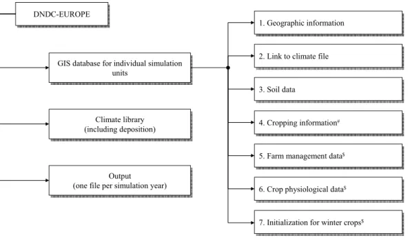
An overview of the link between the two models is given in Fig. 1.

We combine a socio-economic database, defined at the level of administrative re-gions and designed to drive economic model CAPRI, and an environmental database in a geographical information system (GIS) environment, which is mainly used to drive the process-based model DNDC. This database contains also the agricultural land 10

use and livestock density maps, which are derived using econometric methodologies as described in Sect. 2.3. Environmental and land use/management information is used together with the estimates of production levels and farm input (see Sect. 2.4.2) at the scale of the spatial calculation units, which are obtained within the CAPRI mod-elling framework, to define the scenario and set-up the aggregation level and final input 15

database to run the DNDC model (Sects. 2.6). The set of environmental indicators con-tains both data on soil fluxes calculated with the process-based model and emissions from livestock production systems.

2.2 The spatial calculation unit

We chose four delimiters to define a spatial calculation unit, which in the following is 20

also denoted as “Homogeneous Spatial Mapping Unit” (HSMU), i.e. soil, slope, land cover and administrative boundaries. The HSMU is regarded as similar both in terms of agronomic practices and the natural environment, embracing conditions that lead to similar emissions of greenhouse gases or other pollutants.

The HSMUs are built from four major data sources, which were available for the area 25

(9)

BGD

EGU

2004) with about 900 Soil Mapping Units, the CORINE Landcover map (European Topic Centre on Terrestrial Environment, 2000), and a Digital Elevation Model (CCM DEM 250, 2004). Prior to further processing all maps were re-sampled to a 1 km raster map (ETRS89 Lambert Azimuthal Equal Area 52N 10E, Annoni, 2005) geographically consistent with the European Reference Grid and Coordinate Reference System pro-5

posed under INSPIRE (Infrastructure for Spatial Information in the European Commu-nity, Commission of the European Communities, 2004).

One HSMU is defined as the intersection of a soil mapping unit, one of 44 CORINE land cover classes, administrative boundaries at the NUTS 3 level (EC, 2003; Statistical Office of the European Communities (EUROSTAT), 2003), and the slope according 10

to the classification 0 degree, 1 degree, 2–3 degrees, 4–7 degrees and 8 or more degrees. As the HSMU of at least two single pixel of one square kilometre are not necessarily contiguous, we can speak from the HSMU as of “pixel cluster”.

2.3 Estimating agricultural production

2.3.1 Crop levels 15

Statistical information about agricultural production is obtained at the regional NUTS 2 or 3 level from the CAPRI database. This database contains official data obtained from the European statistical offices (available athttp://epp.eurostat.ec.europa.eu) and are checked on their completeness and inherent consistency, and complemented with management data to make them useable for modelling purposes (Britz et al., 2002). In 20

the case of data gaps or controversial data, the problems are fixed with a well defined algorithm staying as close as possible to the original data source.

Data on crop areas are downscaled to the level of the HSMU using a two-step sta-tistical approach combining prior estimates based on observed behaviour with a rec-onciliation procedure achieving consistency between the scales.

25

The first step develops statistical regression models for estimating crop shares (ex-pressed as percentage crop area to total area of the pixel-cluster), simulating the

(10)

prob-BGD

EGU

ability that at a certain point a crop is grown as function of regressed parameters and local landscape characteristics (climate, soil properties, land cover etc.). Those pa-rameters are determined based on the “Locally Weighted Binomial Logit Estimation” technique (e.g. Anselin et al., 2004), estimated with a maximum likelihood estima-tor maximizing the probability that the observations that were obtained from the Land 5

Use/Cover Area Frame Statistical Survey (LUCAS, European Commission, 2003a) are realized. To account for the possibility that other factors than natural conditions influ-ence the choice of farmers to grow a specific crop, the weight of LUCAS observations is discounted with the distance from the respective HSMUs.

The second step determines the first and second moments of a priori estimates of 10

the land use shares for each HSMU and for each of the 29 crops for which statistical information is available. Consistency with the regional statistics is then obtained with the Bayesian highest posterior density estimator (HPD, Heckelei et al., 2005), which allows in a transparent and elegant way to combine different pieces of information, using a covariance matrix calculated according to Green (2000). The results are the 15

most probable cropping and further land use shares at HSMU level which exhaust the area of each HSMU and are in line with given regional crop and land use data or projections.

The area under analysis covers all 27 Member States of the European Union (EU27). As explained above, land cover is one of the delineation factors for the HSMUs which al-20

lowed exclusions of such HSMUs where we assumed that no agricultural cover should be present. However, a rather wide range of land cover classes comprising 11 agricul-tural or mixed agriculagricul-tural CORINE land cover classes and 7 non-agriculagricul-tural classes was maintained. As the definition of a CORINE mapping unit requires a minimum of 25 ha of homogeneous land cover, spatial units might include fractions of other 25

CORINE classes, e.g. we typically find some grassland in forest areas and vice versa. In regions with predominant forest land cover significant percentages of the grassland reported in agricultural statistics might be “hidden” in forest CORINE classes while in regions with prevailing “pasture” according to CORINE this share might be negligible.

(11)

BGD

EGU

The overall procedure tries to eliminate these negligible fractions of land use from the HSMU by manipulating the prior expectations. The statistical procedure is described in more detail in Kempen et al. (2007)1.

2.3.2 Estimating animal stocking densities

Manure availability is linked to livestock density, and we further assume a close link be-5

tween local manure availability and local application rates. In opposite to crops, there is no common Pan-European data base available which comprise at a high spatial res-olution data on animal activity levels, necessary for the estimation of local parameter sets of regression functions for animal stocking densities. Instead, the data on herd sizes from the Farm Structure Survey at NUTS III level (about 1000 regions for EU25) 10

are regressed on data which are available or can be estimated at the level of single HSMUs: crop shares, crop yields, climate, slope, elevation, and economic indicators for group of crops as revenues or gross margins per ha. We will explain below how HSMU specific yields and economic performance indicators are derived. All explana-tory variables are offered in linear and quadratic form as well as square roots to an 15

estimator which uses backward elimination, i.e., continues to exclude variables as long as the adjusted R2is increasing or as long as there are variables which are not equal to zero below the 2.5% significance level. Generally, the estimation is done for single Member States, however, in cases where not enough FSS regions are available for a Member States, countries are grouped during the estimation. The regression is applied 20

to the 14 animal activities covered in the CAPRI data base as well as for livestock unit weighted aggregates for ruminants, non-ruminants and all types of animals. The vast majority of the regressions yield adjusted R2 above 80%. As expected, a low share of explained variance was found in a number of cases for area independent livestock systems (pigs, poultry).

25

1

Kempen, M., Heckelei, T., Britz, W., Leip, A., and Koeble, R.: A Statistical Approach for Spatial Disaggregation of Crop Production in the EU, in preparation, 2007.

(12)

BGD

EGU

Given the fact that the variance of the explanatory variables at HSMU level is far greater then in the FSS region sample per Member States, estimating at single HSMU level would be prone to yield outliers with a high variance regression error. Therefore, expected means for each variable and HSMU are obtained by using a distance and size weighted average of the explanatory variables of the surrounding HSMUs. Equally, the 5

variance of the regression error per HSMU is determined from those HSMU specific averages of the explanatory variables. The resulting expected mean and variance are used as the a priori distribution of a Highest Posterior Density (HPD) estimator, approximating the t-distributed regression results with a normal distribution, so that after taking the logs of the likelihood function a quadratic function to maximise was 10

obtained. The HDP determines those stocking densities at the level of HSMU which simultaneously recover the given herd sizes at the level of FSS region, ensure that the livestock densities per animal type aggregate up to stocking densities for ruminants, non-ruminants, and all types of animals and that the joint posterior density according to the distribution of the regression results is maximized.

15

2.4 Estimating agricultural management

The DNDC model requires the following agricultural management parameters: appli-cation rates and timing of mineral and organic fertilizer, tillage timing and technique, irrigation, sowing and harvesting dates, with more data such as additional information on crop phenology being optional.

20

2.4.1 Potential yield

DNDC simulates the crop growth using a logistic function (S-curve) which tries to obtain maximum obtainable nitrogen uptake and biomass carbon, which is pre-defined, at a daily time step. Partitioning total biomass into the plant’s compartments (root, shoot, grain) at harvesting time is also given as default data in the crop library files (Li et 25

(13)

BGD

EGU

the pre-defined total plant carbon will be realized at harvesting time. If any stress of temperature, water or nitrogen occurs during the simulated crop growing season, a deduction of the biomass will be quantified by DNDC. We used statistical production data at the regional level, yields and area, down-scaled to the scale of HSMUs using information of potential yields for each soil polygon obtained from model simulations 5

with the crop model WOFOST (van Diepen et al., 1989), as input values for the potential yield in DNDC.

The yields at HSMU level were used in the conjunction of input demand factors as applied to build the regional CAPRI data base to derive input coefficients per crop at the level of single HSMUs. Along with NUTS II prices for outputs and inputs, and 10

data on agricultural subsidies, the resulting data set allows the calculation of economic performance indicators for crops at the level of HSMUs, which were used as possible explanatory variables for stocking densities.

2.4.2 Mineral and organic fertilizer application rates

Estimation of nitrogen application rate per crop at the level of HSMUs is based on a 15

spatial dis-aggregation of estimated application rates at regional (NUTS II) level from the CAPRI regional data base. As there are no Pan-European statistics on regional application rates available, the estimation process in CAPRI at NUTS II level is briefly described. The challenge consists in defining application rates which are consistent with given boundary data – national mineral fertiliser use and manure nitrogen excreted 20

from animals –, cover crop needs and lead to plausible distribution of nitrogen losses over crops and regions. The estimation is based on the Highest Posterior Density Esti-mator. Manure nitrogen in a region is defined as the difference between nitrogen intake via feed – either concentrates or regionally produced fodder – and nitrogen removals by selling animal products according to a farm-gate balance approach. Assuming no 25

trade of nutrients across NUTS II boundaries, the available organic nitrogen must be exhausted by the estimated organic application rates. The same holds at the national level for total mineral nitrogen use in agriculture. Estimates at Member State level on

(14)

BGD

EGU

mineral application rate for selected crops or groups of crops are available from the In-ternational Fertilizer Manufacturers Organization (FAO/IFA/IFDC/IPI/PPI, 2002) which provides as well statistics on total mineral fertilizer use in agriculture. The HDP estima-tor is set up as to minimize simultaneously the differences between the estimated and given national application rates and to stay close to typical shares of crop needs cov-5

ered by organic nitrogen and assumed regional surpluses, ensuring via constraints that crop needs are covered and the available mineral and organic nitrogen is distributed. Upper bounds on organic application rates reflecting the nitrate directive are introduced for NUTS II regions comprising nitrate vulnerable zones.

The spatial distribution of the resulting regional application rates to single HSMUs is 10

less demanding as in opposite to the regional distribution, interactions between crops or crop groups are not re-calculated. Based on the estimated crop yields, nitrogen removals per crop are defined and manure nitrogen application rates are estimated per crop and HSMU as described in the following. We estimate first an average of the NUTS II application rate surrounding the HSMU using the inverse distance in kilometre 15

multiplied with the size of NUTS II region in square kilometre as weights. The same weights are used to define the average organic nitrogen available per hectare. The manure application rate per crop in the HSMU is obtained by the multiplication of three terms, i.e. (i) the average organic application rate as defined above; (ii) the relation between the crop specific nitrogen removal at HSMU level and the removal at NUTS II 20

level; and (iii) a term depending on the relation between the organic nitrogen availability per hectare at HSMU level, which is obtained from the animals stocking density in the HSMU, the average manure availability as described above, and the size of the HSMU. The resulting estimated organic application rates per crop and HSMU are scaled with a uniform factor to match the given regional application rates. Summarizing, organic 25

rates at HSMU will exceed average NUTS II rates if yields at HSMU are higher – which lead to higher nitrogen crop removal – or if stocking densities are higher driving up organic nitrogen availability.

(15)

BGD

EGU

the relative surplus estimated at regional level minus the estimated organic applica-tion rate net of ammonia losses and atmospheric deposiapplica-tion. Those estimates are increased in case that assumed minimum application rates are not reached. As with organic rates, a uniform scaling factor lines the HSMU specific estimates up with the regional ones.

5

2.4.3 Crop sowing and harvesting dates

Crop sowing and harvesting dates are obtained from Bouraoui and Aloe (2007).

2.4.4 Number and timing of fertilizer and tillage

Number and timing of fertilizer and tillage applications is taken from the DNDC farm library (Li et al., 2004) taking for good the dates relative to sowing or harvesting and 10

applying these time lags to the actually simulated sowing or harvesting dates, respec-tively.

2.4.5 Irrigation

The DNDC model treats irrigation such that a calculated water deficit is re-plenished to a pre-defined percentage. Irrigated cultures do not suffer any water deficit, while non-15

irrigated cultivation will feel water-stress when water demand by the plants exceeds the water supply. Percentage of irrigated area was calculated on the basis of the map of irrigated areas (Siebert et al., 2005), and was taken as fixed for all crops being cultivated within an HSMU.

2.4.6 Other management data 20

All other information needed to describe farm management and crop growth, such as tillage technique, maximum rooting depth and so on are taken from the DNDC default library and used as a constant for each crop for the whole of the simulated area.

(16)

BGD

EGU

2.5 Environmental input data

2.5.1 Nitrogen deposition

Data on nitrogen concentration in precipitation was obtained from the Co-operative Programme for the Monitoring and Evaluation of the Long-Range Transmission of Air Pollutants in Europe (EMEP, 2001). EMEP reports the data as precipitation weighted 5

arithmetic mean values in mg N L−1 _{as ammonium and nitrate measured at one of the} permanent EMEP stations. We used the European coverage processed by Mulligan (2006).

2.5.2 Weather data

Daily weather data for the year 2000 were obtained from the JRC (MARS). The data 10

originate from more than 1500 weather stations across Europe, which were spatially interpolated onto a 50 km×50 km grid by selecting the best combination of surrounding meteorological stations for each grid (Orlandi and Van der Goot, 2003).

2.5.3 Soil data

A series of 1 km×1 km soil rasters has been processed using pedo-transfer rules on 15

the basis of the European Soil Database2(Hiederer et al., 2003).

The DNDC model requires initial content of total soil organic carbon data (SOC) in kg C kg−1 _{of soil including litter residue, microbes, humads and passive humus} in the topsoil layer, clay content (%), bulk density (g cm−3_{) and pH. The database} contains under others rasters of topsoil organic carbon, texture, packing density, and 20

base saturation. The latter two had been processed by Mulligan (2006) to obtain dry bulk density and pH, respectively, using linear relationships.

2

(17)

BGD

EGU

Soil organic carbon content has been derived using an extended CORINE land cover dataset, a digital elevation model (DEM) and mean annual temperature data (Jones et al., 2005). As DNDC has been parameterized for mineral soils, we restricted the simulations to spatial units with a topsoil organic content of less than 200 t ha−1(Smith et al., 2005a).

5

2.6 Model set-up

2.6.1 Adaptation of the model

Using the default version it was not possible to accommodate the degree of flexibility that was required in our study. Necessary adaptations regarded data handling; param-eterization of the processes was according to (Li et al., 2004). First, it was necessary 10

to allow for each modelling unit an individual number and selection of crops that are simulated; second, farm data such as fertilizer application rates are calculated indi-vidually for each simulation unit. In the default version of DNDC, the farm library is constant at province level. Third, potential yield is determined for each modelling unit; in the default version of DNDC the crop libraries are constant at national level. Last, 15

for easier post-processing of the data, output files were grouped into single tables for each simulation year.

2.6.2 Set up of the simulation

The above-defined HSMU can be regarded as the smallest unit on which simulations can be carried out. This, however, is not always practical, as the high number of units 20

is combined with a number of scenarios or if a multi-year simulation is carried out. Therefore, an intermediate step re-aggregates the HSMUs for each scenario that is simulated by the model, into model simulation units (MSUs) on the basis of both agro-nomic and environmental criteria. In this way, the design of the scenario calculations can be best matched with the objectives of the study.

(18)

BGD

EGU

In our study, the objective of the simulation was to cover as much variability as pos-sible in order to enable to assess the impact of the environment (represented in the model by daily weather data and soil parameters) and cultivation patterns. Therefore, for each region defined in the economic model (NUTS II), all crops that cover at least 5% of the agricultural area are included in the model. These crops were simulated 5

on MSUs that had a crop share of more than 35% of the agricultural area within an agricultural unit (defined by a minimum of 40% of the area used for agriculture) or the crop share was at least 85% of the maximum share of the crop occurring in the re-gion. Before eliminating single units, however, all units were clustered according to their similarity in the environmental conditions. To this purpose, a tolerance is defined 10

for each parameter that gives the maximum spread allowed within a single cluster. For example topsoil organic matter content was clustered if the values differed less than ±10%. The thresholds and tolerances used in this study are listed in Table 1. These moderate tolerances for soil conditions lead to an average number of more than 68 (up to 266) different soil conditions that were distinguished in each region, with add 15

to 11 438 environmental situations for EU-15, out of which 6391 MSU were simulated with a total of 11 063 crop-MSU combinations. Each of these simulations runs over 99 years to smooth out unrealistic estimates for topsoil organic carbon in the original map. We had complete information for 14 European countries, members of the European Union by 2004: Austria, Belgium, Finland, France, Germany, Greece, Luxembourg 20

(simulated as part of Belgium), Italy, Netherlands, Portugal, Spain, Sweden, United Kingdom. Statistical and weather information were centred on the year 2000. HSMU data for Ireland and the countries that joined the European Union in 2004 or 2007 have also been processed but are not yet included in the current simulation run. We simulated the following crops: cereals (soft and durum wheat, barley, oats, rye, maize, 25

and rice), oil seeds (rape and sunflower), leguminous crops (soybean, pulses), sugar beets, potatoes, vegetables and fodder production on arable land.

We performed several scenario calculations to investigate the model’s response to fertilizer input. Therefore, each simulation using the most probable management data

(19)

BGD

EGU

estimated as described in Sect. 2.4.2 was repeated without any input of mineral fertil-izer or manure nitrogen. Additionally, each scenario was calculated under irrigated and non-irrigated conditions. The most probable situation is then calculated on the basis of the irrigation map described in Sect. 2.4.5 as a weighted average under irrigated and non-irrigated conditions. Simulation results were aggregated to the scale of the regions 5

or countries as area-weighted averages.

3 Results

3.1 Homogeneous Spatial Mapping Units

The HSMUs cover a wide range of sizes from a minimum area of 1 km2but some reach very large areas (up to 9723 km2) in regions with a homogeneous landscape in terms of 10

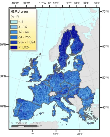
land cover and soil. The mean area of a homogeneous spatial mapping unit, indicates the range of environmental diversity with regard to land cover, administrative, data, soil and slope, and ranges from 7 km2for Slovenia to 94 km2for Finland with an European average around 21 km2(see Table 2 and Fig. 3). In total, a number of 206 000 HSMUs cover almost 4.3 million km2 in Europe. Small discrepancies in the surface area of 15

countries stem from rounding errors during the re-sampling procedure and are higher in areas with a high geographical fragmentation (i.e., small islands, complex coastlines or borders). For EU27 we obtained in total about 138 000 HSMUs in which agricultural activities (arable land and grassland) occur, occupying about 77% of the European landscape.

20

3.2 Land Use and livestock density maps

Figure 4 shows a summary of the land use and livestock density maps as total agri-cultural area (UAAR) and total livestock units (LU/ha) in Europe. The figures are su-perimposed to a hill-shade and show the relationship of topography and UAA. In these

(20)

BGD

EGU

spatial units the average area used for agriculture amounts to 47%, ranging from 8% in Finland and Sweden to more than 70% in the United Kingdom and Ireland. Differences are found between the “old” Member States (EU15), being a member of the European Union already before 1 May 2004 and the “new” Member States that became member of the EU at or after this date (EU12). For EU15, the 75% of the area belongs to a 5

spatial unit with some agricultural use and only a little bit more than half of the area has agricultural use of more than 5%. EU12 countries have less intensive agricultural systems, and most of the surface is covered by HSMUs with some agricultural use (89%) and only 20% of the surface area has less or equal than 5% of agricultural land use. Other examples of agricultural land use maps obtained are shown in Fig. 5 for 10

barley and permanent grassland for the year 2000.

The livestock density maps highlight the huge variance in stocking densities found in Europe linked to differences in farming systems and natural conditions. Highest stock-ing densities are found in parts of The Netherlands, Belgium, some German counties close to The Netherlands and Belgium, Bretagne and the Po flat in Italy. In all those 15

cases, mixed farming systems are found both featuring ruminants and non-ruminants, and fattening processes based on concentrates. The lowest stocking densities are linked to regions were specialized crop farms are the main production system, often found where over time large-scale arable farming under favorite conditions developed. A classical example is the French plain north of Paris. Where heritage laws or other 20

factors favored the development of smaller farms, a low land-to-man ratio rendered it useful to generate added value to crop products by fattening processes. Here, stocking densities are often in average ranges, and where part-time farming is prevalent, have declined over time.

Despite the strong link between permanent grass land and ruminants, the link be-25

tween stocking densities and grass land shares is not obvious as stocking densities in grass land regions depends to a large extent on grass land productivity. In mountain-ous areas, low grass land yields typically lead to semi-natural grass lands with rather low stocking densities. The same holds for regions with very low average temperature,

(21)

BGD

EGU

and in some cases, for regions with low rainfall under rainfed farming conditions. How-ever, as statistics or land use cover maps may not account semi-natural grass land as Utilizable Agricultural Area, the stocking density map may show a combination of higher stocking densities and lower shares of agricultural area in some regions, where in reality, lower stocking densities are linked with semi-natural grass land.

5

Local hot spots are possible almost everywhere with area independent farming sys-tem e.g. laying hens or fattening of pig or poultry. Albeit environmental legislation requires in most countries a certain land base for manure disposal, it is often sufficient for farmers to have a contract with other landowners allowing them to spread manure on fields not primarily managed by them. That renders is somewhat difficult to link di-10

rectly farming structure and manure management practise. Accordingly, as discussed above, organic application rates are linked to manure availability in larger areas.

3.2.1 Validation of the land use maps

Error assessment analyses of the agricultural land use maps have been performed both at the regional scale, using district-to regional scale from an agricultural census of the 15

year 2000 covering the EU15 member states and at the local scale, using commune-level statistics of the Lombardia region in Italy and the Netherlands.

The economic model CAPRI uses statistical information for agricultural land use for NUTS II regions. Therefore the initial distribution of the different crops to the individual HSMUs was performed based on NUTS II agricultural statistics.

20

These results were compared with the data from the agricultural census of the Eu-ropean Union, the Farm Structure survey (FSS2000, EuEu-ropean Commission, 2003b). For some European regions, land use statistics from the FSS2000 is available at a lower administrative level, NUTS III. Within the area where both data sets were avail-able (see Fig. 6) the NUTSII regions are subdivided in minimum 2 and maximum 10 25

NUTSIII regions. This information is used as out-of-sample observation to assess the errors of the results of the dis-aggregation algorithm.

(22)

BGD

EGU

III level and compared with the FSS2000 statistics as out of sample data. For each single crop the difference between the crop area given by FSS2000 and the area of the dis-aggregation result was calculated. All positive area differences were summed up for all crops and expressed as percentage of the total NUTS II agricultural area. In this way we obtain the share of misclassified agricultural area in a NUTS II region which is 5

shown Fig. 6 for all regions where FSS2000 data on NUTS III level was available. In addition the pie charts give the contribution of each crop to the total error.

The misclassified agricultural area within NUTS II regions ranges between 2% and 35. With the developed dis-aggregation procedure very good results (2–15% misclas-sified area) have been obtained for the UK, Ireland, France and Southern Spain. The 10

errors are slightly higher in Northern/Central Spain and Portugal. For Southeastern Italy, Greece and some regions in Sweden and Finland errors of about 25–35% oc-cur. The higher errors in Sweden and Finland can be explained by the very small agricultural area which has to be located in quite large HSMUs. Higher errors can be the result of the dis-aggregation procedure which might be not appropriate for some 15

regions but can be also a consequence of inaccuracies and inconsistencies in the in-put data for the dis-aggregation (CORINE land use/cover, LUCAS survey, agricultural statistics etc). We obtain an area weighted mean error of ∼12.2% for Europe (area considered; see Fig. 6).

Very rarely single crops are considered in a model exercise or in other applications. 20

Usually the crops are grouped according to their physical similarity or the demand for analog agricultural practices. If we consider only crop groups (cereals, fallow land, rice and oilseeds, industrial crops, permanent crops and grassland and fodder), some of the distribution errors level out as within these groups requirements of the plants to the site conditions are sometimes very similar and cannot easily be distinguished 25

by the model. For the countries included in the calculation, the dis-aggregation error decreases from 12% for individual crops to 8% for crop groups. The error of very coarse crop classes (arable crops, permanent crops and grassland and fodder) is still lower (6.2%) and 3.4% of the total UAA was attributed to wrong NUTS III regions.

(23)

BGD

EGU

However, applying no dis-aggregation, and simply distributing the NUTS II crop shares homogeneously over the corresponding NUTS III regions, would result in twice as much mis-classified area, i.e. 24%. Looking more in detail at the NUTS II level the “no dis-aggregation” case yields large errors of 40 to 50% for a number of cases mainly in France, Spain, and Italy. Only in a few cases we find that the dis-aggregation of the 5

data yield a larger error than the even distribution over the NUTS III regions. The re-gion Pohjois in Finland, for example, is the only rere-gion where the dis-aggregation result yields an error above 30% of the agricultural area, which is with 35.6% slightly worse than the even distribution (32.6%). The only large discrepancy is found in (Mellestra Norrland) where the crop shares in the two NUTS II regions is very close to the mean 10

distribution (error 4.7%) and the dis-aggregation produced an error of 18%.

Error assessments of the agricultural land use maps have also been performed at the local scale, using commune-level statistics for the year 2003 of the Lombardia region in Italy (ERSAF, 2005) and the Netherlands. The latter, however, will not be presented here.

15

For the Lombardy region, we compared the rice and maize distribution in 190 com-munes with the results of the aggregation. For illustration, Fig. 7 shows the dis-aggregation result (1 km by 1 km grid resolution) and the maize fields based on ERSAF (2005) data for a set of communes. The maize pattern (light brown areas) indicating a maize share of 30–60% from the dis-aggregation result corresponds with the main 20

maize field distribution based on ERSAF. But looking at the scatter plot (Fig. 8a) com-paring ERSAF and dis-aggreation data for maize in all 190 communes it can be seen that generally the dis-aggregation blurs the distribution that is more distinct in reality. For the interpretation of this comparison, however, one has to keep in mind that the areas of the single communes are close to the mean HSMU area in this region, some-25

times even larger. Our approach does not allow distributing crop area below the HSMU level and therefore some discrepancies are unavoidable. Thus, we reach herewith the maximum level of detail that can be considered. Furthermore, maize is a crop that has no single corresponding CORINE land cover class in which it occurs but is distributed

(24)

BGD

EGU

over range of classes. The contrary holds for rice as a separate class rice fields is given in CORINE, thus the dis-aggregation result for rice (Fig. 8b), corresponds closely to the communal data.

3.2.2 Validation of the livestock density map

The data set resulting from the distribution algorithm of the animal activities was vali-5

dated using out-of-sample data available for France at the level of 36 000 communes from the Farm Structure Survey. The individual herd sizes shown per commune were aggregated to livestock units. The results obtained for the about 24 000 pixel clusters for France were averaged per commune, and the absolute error in the stocking densi-ties calculated. A result of e.g. 0.5 indicates that the area weighted average livestock 10

density of the HSMUs polygons intersecting the polygon of the commune is 0.5 live-stock units per ha higher then the data reported in the French Farm Structure survey. The resulting map is shown in Fig. 9a. The errors are classified in 5% quantiles, so that according to the legend, in 90% of the communes, the error in estimating the stocking estimating is between −0.46 or +0.43 livestock units per. In 80% of the communes, the 15

errors is between −0.28 and +0.31 livestock units per ha.

Those errors were compared with estimates per communes using the NUTS III av-erage livestock density, with errors shown in Fig. 9b. Those livestock densities are the boundary data to which the results of the HSMUs in that NUTS III region had been consolidated. It can be seen that the statistical estimator for the livestock densities 20

yields results which are somewhat similar to using NUTS III averages. However, when comparing the quantiles of the error distribution, it is obvious that the error distribution of estimator is more peaked as can be also seen from the distribution diagrams shown in the figures, i.e. the number of communes with a small differences between the ob-served and the estimated stocking densities is higher for the estimates compared to 25

using average NUTS III livestock densities. Further on, the map with the errors from using the NUTS III livestock densities shows a sharper clustering of errors in space. That observation is important as organic fertilizer applications for a specific HSMU

(25)

BGD

EGU

are generated inter alia depending from a distance and size weighted average of sur-rounding HSMUs. When errors are clustered in space, averaging over HSMUs will not reduce errors, whereas with a high variance of errors in space, especially if HSMUs with under- and overestimated stocking densities are near to each other, averaging will reduce the overall error.

5

3.3 Results input data

3.3.1 Nitrogen application

On average 106 kg N of mineral fertilizer are applied per hectare to the agricultural land in Europe, and 61 kg N contained in manure. Hence, the share of manure nitrogen in the total nitrogen application is 37% which is similar to the share reported in the 10

national greenhouse gas inventory of the European Communities of 33% (EEA, 2006). There are obviously large differences between the different countries, according to the intensity of livestock production as well as between the crops. Table 3 shows the average national nitrogen application rates for mineral fertilizer and manure by crop. Belgium, Denmark and The Netherlands are able to cover most of the nitrogen needs 15

by using manure; France, Portugal and the United Kingdom must purchase most of the applied nitrogen from mineral sources.

The low average manure application rates in countries for France, Portugal and United Kingdom can be explained by several factors. First of all, compared to Bel-gium, Denmark and the Netherlands, the average livestock densities are considerable 20

lower. Secondly, stocking densities are dominated by ruminants which are linked to grass land. And thirdly, especially in France and the UK the main arable cropping regions are dominated by specialized farms without animals.

(26)

BGD

EGU

3.3.2 Export of nitrogen with harvested material

The uptake of nitrogen by the plants is the largest single pathway of nitrogen added or recycled during a year. With an average of 233 kg N ha−1 y−1 for all countries and crops simulated it balances approximately the total input of nitrogen by fertilizer application, nitrogen fixation and nitrogen deposition (217 kg N ha−1_y−1_{; see Table 4).} 5

The ratio of nitrogen uptake to nitrogen delivery is highest for cereals such as rye and barley where twice as much nitrogen is contained in the plant than was added to the system. Sunflower and paddy rice, on the other hand, were taking up only a half of the offered nitrogen. Obviously, a large part of the nitrogen that accumulates in the biomass will remain in the system, as only a – crop-dependent – fraction will be 10

removed at harvest. Also, recycling of nitrogen in the soil (mineralization of organic matter and crop residues) contributes differently to the pool of available nitrogen.

For all crops considered the amount of nitrogen in the harvested material amounts to 40% to 70% of the total plant nitrogen. For the above-ground biomass which is not harvested, it was assumed that 90% of the crop residuals were left on the field (Li et 15

al., 1994). These numbers suggest a simulated nitrogen surplus between 15% for oats and more than 80% for sunflower. Nitrogen surplus pathways will be discussed in more detail in Sect. 3.4.

As described above, nitrogen application rates are calculated as a function of the estimated (aboveground) nitrogen uptake. This information is translated into potential 20

total plant carbon to be achieved without environmental stress. Generally, the reduction in assimilated plant carbon respective to the optimal situation is relatively stable for the different crops. Looking at all simulations, we achieved only a plant biomass of 66% of the potential value. Most cereals (soft wheat, durum wheat, rye and barley) range at approximately 70%–80% of the optimal yield, with maize and durum wheat 25

scoring lowest. These crops achieved only half of the potential biomass, similar to potatoes and sugar beet. Paddy rice and soya were closest to their potential biomass carbon (approximately 90%). In most of the cases, the model was able to achieve

(27)

BGD

EGU

the pre-defined distribution of carbon over the plant compartments (root, shoot and grain), which shows that the phenology given to the model (sowing and harvest dates) corresponds to the parameterization of plant development. Problems were observed only for crops growing in Finland, where the maturation of the plants was simulated too slowly resulting in larger fractions of carbon to be allocated in root and shoot. For 5

example, only 17% of the carbon was contained in the grain of soft wheat at harvest, which is about half the target value, while carbon in roots and shoot was much higher.

3.3.3 Topsoil organic carbon content

Net mineralization of organic matter in soils and assimilation of mineral nitrogen into organic matter are processes that occur mainly in systems that are in a phase of tran-10

sition between two different land management systems. In the model world, land use transitions can be studied applying appropriate initial conditions of the soil parameters. We simulated a loss of soil organic matter of 25% or 23 t C ha−1_{during 100 years using} the same weather and management data. Losses were highest in the first simulation years with an average loss of 0.5 t C ha−1 _y−1 _{during the first decade slowing down} 15

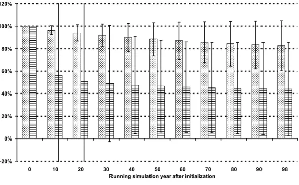
to 0.1 t C ha−1 _y−1 _{during the last decade. The latter value is close to estimates of} current carbon losses from European croplands (Vleeshouwers and Verhagen, 2002). The dynamics of carbon losses are following a first-order decay with a time constant of 0.3% y−1_{. The dynamics of soil organic carbon during the simulation period is shown} in Fig. 10 (dotted symbols) for the average relative decrease of soil organic carbon 20

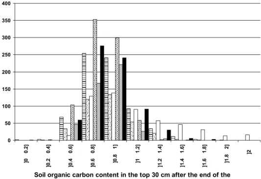
content over all spatial simulation units. After 99 simulation years, soil organic carbon stocks reached 82%±22% of the initial values corresponding to a decrease of the av-erage soil organic carbon stocks in the top 30 cm of the soil from 93±45 t C ha−1 _to 70±30 t C ha−1_{. Note that the decrease of the average carbon stocks is steeper (down} to 75%), which is due to a few (10%) spatial units with high soil organic carbon content 25

that lost 40% or more of their initial carbon. On the other side, 15% of the simulation showed an increase of soil organic carbon. The distribution is thus slightly skewed, which is also shown in Fig. 11 presenting the distribution of relative changes for

(28)

se-BGD

EGU

lected crops. Significant increases in soil organic carbon of more than 50% occurred of the initial value only for maize in ca. 15% of cases. For all crops, the highest number of cases was observed in the classes between 0 and 10% or between 10 and 20% reduction of organic carbon during the 100-year simulation runs.

The dashed symbols in Fig. 10 show the impact of the declining soil organic matter 5

content on the simulated N₂O fluxes relative to the initial situation over all simulated spatial modeling units. The average N₂O flux declines faster than the average rela-tive N₂O flux in the single spatial modeling units, as we have seen also for the carbon stocks; while initial N₂O fluxes were 17 kg N-N₂O ha−1 _y−1_{, they reduced after 100} simulation year to 2.8 kg N-N₂O ha−1 _y−1_{corresponding to only 16% of the initial N}

2O 10

flux simulated. Variability is very high throughout the years, even though decreasing with time. The average relative decrease shown in Fig. 10 over the units is only down to 44%. This suggests that some un-realistically high topsoil organic carbon estimates lead to extremely high N₂O fluxes in the first simulation years (even fluxes of 100 kg N-N₂O and more were simulated under initial conditions), which declined quickly di-15

minishing their weight in the mean N₂O flux. The standard deviation of the average decrease of the relative N₂O flux is 200% in the tenth simulation year reflecting the same fact that large reductions in a few modeling units and smaller reduction in a higher number of modeling units occurred. N₂O fluxes and standard deviation of mean N₂O fluxes are relatively stable after 50 simulation years with an average decrease of 20

0.05% y−1_{which reduces to 0.04% y}−1 _{during the last simulated decade.} 3.4 Simulation results

All results presented in this section are related to the last simulation year, i.e. after 99 years of simulating the same management and climate situation.

Being a comprehensive biogeo-chemical model of nutrient turnover in agricultural 25

soils, DNDC calculates all elements in the nitrogen balance in soils. Being a method-ological paper, we restrict here to present the simulated nitrogen budget at national

(29)

BGD

EGU

scale. Table 4 shows a summary of the quantified, i.e. reported elements in the N budget aggregated to the country scale. Outputs of nitrogen by nitrogen losses and export of plant material either of plant products or crop residues is opposed to the input of nitrogen via nitrogen application, deposition, fixation, and release of nitrogen trough net mineralization of soil organic matter. Net mineralization of organic matter leads in 5

some countries to a loss of nitrogen, if soil organic matter has been simulated to build up in that country. The two sides of the balance are large fluxes of nitrogen and cover a large range between 77 kg N ha−1 _y−1_{(Greece) to 430 kg N ha}−1_y−1_{(Belgium). The} export of nitrogen with the crop has been calculated as the residual from the difference of nitrogen in- and outputs to close the nitrogen budget at the soil surface. There might 10

be errors due to unaccounted sources or sinks of nitrogen in the simulations, such as allocation of biologically fixed nitrogen in soil compartments or leaching of organic mat-ter. However, these are considered to be minimal, as was found in simulations where crop development was suppressed. Here the nitrogen balance was close to zero within the bound of the rounding errors. Also, C/N ratios of the exported plant biomass was 15

in most cases identical or slightly higher (due to the higher C/N ratio in plant shoot biomass) to the pre-defined C/N ratios in grain. Presumably therefore, the error in-troduced by using a constant C/N ratio for mineralized soil organic matter was small. DNDC knows different pools of organic matter with defined C/N ratios. The C/N ratio of litter varies from very labile (C/N=5) over labile (C/N=50) to resistant litter (C/N=200). 20

Other compartments comprise microbial biomass, humads and humus, which are all characterized by a C/N ratio of 12.

The nitrogen surplus generally is an important indicator for defining the environmen-tal impact of agriculture on one hand and the effectiveness of environmenenvironmen-tal policies on the other hand. Calculating nitrogen surplus as the ratio of nitrogen not taken up 25

by plants (both in harvested material or in removed crop residues) to the total nitrogen input during the simulation year, it ranges between 26% (United Kingdom) and 55% (Italy). The value calculated for all countries considered is 38% nitrogen surplus.

(30)

BGD

EGU

4 Discussion

4.1 Spatial simulation units

Regional or (sub)continental modeling studies often run their model on a regular grid of varying size depending on the area covered by, the format of available data sets, and the scope of, the simulations. Roelandt et al. (2006) for example aimed at predicting 5

future N₂O emissions from Belgium relying on climate scenarios that were available for a 10′ _{longitude and latitude grid; also Kesik et al. (2005b) linked the simulation} of nitrogen oxides emissions from European forest soils to the available climate data set and run the model on a 50 km×50 km raster. Vuichard et al. (2007) estimated the greenhouse gas balance of European grasslands, due to computing limitations they 10

restrict the simulations to a 1◦ _{by 1}◦ _{degree grid. These approaches are efficient in} fast responses for possible developments or delivering a first estimate of large-scale emissions. For detailed analysis, however, they lack the link to realistic land use data (Roelandt et al., 2006) and are too coarse for capturing local heterogeneities (Vuichard et al., 2007). For a better representation of land use, many authors run their models 15

within the administrative boundaries, for which regional statistics are available. Exam-ples of this approach include simulation studies on about 2500 Chinese counties to estimate soil organic carbon storage (Tang et al., 2006) or greenhouse gas emissions from rice cultivation (Li et al., 2006) using the DNDC model. To assess regional hetero-geneity, the most sensitive factor (MSF) is used giving a reasonable range of emission 20

values with a high probability to cover the true value. This “administrative approach” is also used if the study aims to give support to, or for comparison with, national green-house gas estimates performed with the IPCC emission-factor approach (e.g., Brown et al., 2002; Del Grosso et al., 2005; Mulligan, 2006). Mulligan points out, however, that most of the uncertainty in the emission estimates stem from the large range of 25

environmental conditions encountered within the single modeling units.

To overcome these problems, other studies decided to use the geometry of the avail-able information on soil properties for the delineation of the modeling units used. For

(31)

BGD

EGU

large-scale application as in Grant et al. (2004) to assess the impact of agricultural management on N₂O and CO₂ emissions in Canada, representative soil type – soil texture combinations were defined covering the seven major soil regions in Canada.

Changes in soil organic carbon stocks or fluxes of greenhouse gases were estimated on a basis of landscape units being an intersection of a land-use map and a soil map 5

for Belgium (Lettens et al., 2005) or a region in Germany (Bareth et al., 2001). An additional intersection with a climate map was done in a study on N₂O emissions from agriculture in Scotland (Lilly et al., 2003). These very detailed analyses, however, were so far restricted to relatively small countries or regions due to limitations of computing resources.

10

Schmid et al. (2006) describe a very detailed approach to simulate soil processes in Europe with the biophysical model EPIC. By intersecting landscape variables that are considered stable over time (elevation, slope, soil texture, depth of soil, and volume of stones in the subsoil) they obtained a layer of more than 1000 homogeneous response units. Each of these units was divided, on the average, into 10 individual simulation 15

units by overlaying various maps such as climate, land cover, land use/management and administrative boundaries. Individual simulation units are then regarded as a rep-resentative field site and estimated field impact from simulated management practices are uniformly extrapolated to the entire unit.

The approach described in the present study has many similarities to the HRU/ISU 20

approach described by Schmid and co-workers, as in both cases the philosophy is to develop a framework integrating both environmental and socio-economic impacts on soil processes. The main differences, however, are

– Selected soil characteristics are used to delineate the homogeneous response units by Schmid et al. (2006), while each geometrical unit of the soil database 25

(the so-called soil mapping units) is maintained in the delineation of the homo-geneous spatial mapping units defined here. Each soil mapping unit is a unique combination of one or several soil types. Preliminary land use simulations sug-gested that soil type is an integrative characteristic with relevance for both the