Algorithmic and Implementation Aspects of
On-line Calibration of Dynamic Traffic Assignment
MASSACHUSETTS INSTl
by
_ OFTECHNOLOYEnyang Huang
JUL 15
2010
B.E. Software Engineering
L BRARI ES
School of Computer Science and Engineering
The University of New South Wales
-
Sydney
-
Australia
(2007)
Submitted to the Department of Civil and Environmental Engineering
in partial fulfillment of the requirements for the degree of
ARCHIVES
Master of Science in Civil and Environmental Engineering
at the
MASSACHUSETTS INSTITUTE OF TECHNOLOGY
June 2010
@
Massachusetts Institute of Technology 2010. All rights reserved.
A uthor .... . ... ... ...
Department of Civil and Environmental Engineering
March 31, 2010
Certified by... ... . ... ... ..
Moshe E. Ben-Akiva
Edmund K. Turner Professor of Civil and Environmental Engineering
Thesis
pervisor
A ccepted by ...
- .e .... ...
Daniele Veneziano
Chairman, Departmental Committee for Graduate Students
Algorithmic and Implementation Aspects of On-line
Calibration of Dynamic Traffic Assignment
by
Enyang Huang
Submitted to the Department of Civil and Environmental Engineering on March 31, 2010, in partial fulfillment of the
requirements for the degree of
Master of Science in Civil and Environmental Engineering
Abstract
This thesis compares alternative and proposes new candidate algorithms for the on-line calibration of Dynamic Traffic Assignment (DTA).
The thesis presents two formulations to on-line calibration: 1) The classical state-space formulation and 2) The direct optimization formulation. Extended Kalman Filter (EKF) is presented and validated under the state-space formulation. Pattern Search (PS), Conjugate Gradient Method (CG) and Gradient Descent (GD) are pre-sented and validated under the direct optimization formulation. The feasibility of the approach is demonstrated by showing superior accuracy performance over alternative DTA model with limited calibration capabilities.
Although numerically promising, the computational complexity of these base-line algorithms remain high and their application to large networks is still questionable. To address the issue of scalability, this thesis proposes novel extensions of the afore-mentioned GD and EKF algorithms. On the side of algorithmic advancement, the Partitioned Simultaneous Perturbation (PSP) method is proposed to overcome the computational burden associated with the Jacobian approximation within GD and EKF algorithms. PSP-GD and PSP-EKF prove to be capable of producing predic-tion results that are comparable to that of the GD and EKF, despite achieving speed performance that are orders of magnitude faster. On the side of algorithmic imple-mentation, the computational burden of EKF and GD are distributed onto multiple processors. The feasibility and effectiveness of the Para-GD and Para-EKF algorithms are demonstrated and it is concluded that that distributed computing significantly increases the overall calibration speed.
Thesis Supervisor: Moshe E. Ben-Akiva
Acknowledgments
Thank you to Professor Moshe Ben-Akiva. It has been a great privilege to be able to work with you at MIT. Your knowledge and insights on behavior-oriented traffic simulation have constantly inspired me in my research.
Thank you to Professor Constantinos Antoniou for your encouragement and pa-tience. This thesis is as much a product of your guidance and advice as it is my
effort.
Thank you to Dr. Ramachandran Balakrishna and Dr. Yang Wen for laying the foundation for DTA model calibration. Your ideas and work in this area have greatly inspired me. Thanks for your guidance.
Thank you to the MIT Schoettler Fellowship and the MIT-Portugal program for providing financial support for my graduate studies at MIT.
To my academic advisor, Professor Joseph Sussman, and to my program chair Professor Nigel Wilson, thank you for guiding my academic progress at MIT. To Dr. George Kocur, thanks for your advice and mentoring. To Kris Kipp and Jeanette Marchocki, thank you for your help and advice. To my friends and colleagues in Portugal, Jorge Lopes, Carlos Azevedo, Professor Francisco Camara Pereira and many others, it has been a great pleasure working with you. Our collaboration has achieved great things.
To my lab mates at the Intelligent Transportation Systems laboratory at MIT, Dr. Charisma Choudhury, Dr. Maya Abou-Zeid, Cristian Angelo Guevara, Lang Yang, Ying Zhu, Samiul Hasan, Zheng Wei, Sujith Rapolu, Anwar Ghauche, Hongliang Ma, Li Qu, Nale Zhao, Swapnil Shankar Rajiwade, Martin Milkovits as well as my friends from other laboratories, thank you for accompanying me in this journey. May our friendships last forever.
I would also like to mention a few people who have made my MIT experience possible. Dr. Bernhard Hengst, Dr. William Uther and Dr. Toby Walsh, thank you. Finally, unbounded thanks to Tina Xue from Harvard University for perfecting this thesis. Any remaining errors are my own.
Contents
1 Introduction 17
1.1 Thesis Motivation and Problem Statement . . . . 18
1.2 Sensory Technology State-Of-The-Art . . . . 20
1.3 Dynamic Traffic Assignment Framework . . . . 23
1.4 Literature Review . . . . 27
1.4.1 Calibration for off-line applications . . . . 27
1.4.2 Calibration for on-line applications . . . . 29
1.5 Thesis Contributions . . . . 31
1.6 Thesis Outline . . . . 32
2 Online Calibration Framework 33 2.1 Overview of Framework.. . . . . . . . 34
2.1.1 In-direct Measurement.. . . . . . . . 34
2.1.2 Direct Measurement . . . . 36
2.1.3 System Inputs and Outputs . . . . 36
2.2 Problem Formulation... . . . . . . . . . . . . 38
2.2.1 N otation . . . . 38
2.2.2 Measurement Equations . . . . 38
2.2.3 State-Space Formulation... . . . . . . . . . 39
2.2.4 Direct Optimization Formulation . . . . 41
2.3 Characteristics . . . . 42
2.3.1 Sensor Type . . . .. . . . . . 42
2.3.3 Stochasticity . . . . 43
2.3.4 High Cost Function Evaluation . . . . 44
2.4 Sum m ary . . . .. 44
3 Solution Algorithms 47 3.1 Introduction . . . . 48
3.2 Algorithm Selection Criteria . . . . 48
3.3 State-Space Formulation . . . . 50
3.3.1 Extended Kalman Filter Algorithm . . . . 50
3.4 Direct Optimization Formulation . . . . 52
3.4.1 Categorization on Minimization Algorithm . . . . 52
3.4.2 Hooke-Jeeves Pattern Search Algorithm . . . . 55
3.4.3 Conjugate Gradient Algorithm . . . . 57
3.4.4 Gradient Descent Algorithm . . . . 59
3.5 Sum m ary . . . . 63
4 Scalable Framework Design 65 4.1 O verview . . . . 66
4.2 Scalable Algorithm on Single Processor. . . . . .. 66
4.2.1 The Idea of Simultaneous Perturbation . . . . 67
4.2.2 The PSP-EKF Algorithm . . . . 68
4.2.3 The PSP-GD Algorithm . . . . 70
4.3 Scalable Algorithm on Multiple Processors . . . . 72
4.3.1 Background . . . . 72
4.3.2 Architecture... . . . . . . . . . 74
4.3.3 Definition... . . . .. 75
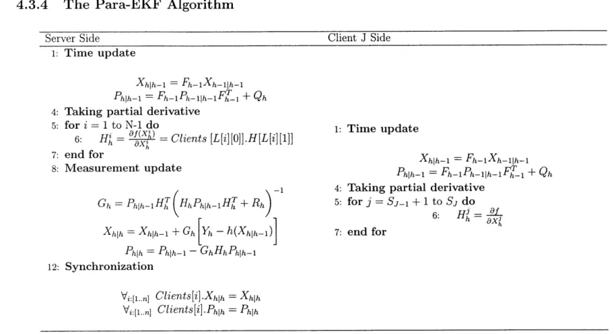
4.3.4 The Para-EKF Algorithm . . . . 76
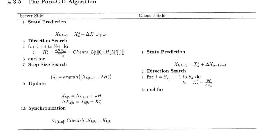
4.3.5 The Para-GD Algorithm.. . . . . . . . 77
4.4 Sum m ary . . . . 78 8
5 Case Study 79
5.1 Objectives . . . . 80
5.2 Experiment Setup.. . . . . . . 80
5.2.1 Network and Sensors . . . . 80
5.2.2 DynaMIT-R . . . . 82
5.2.3 Parameters and variables . . . . 82
5.2.4 Experiment Design . . . . 83
5.3 R esults . . . . 84
5.3.1 Offline Calibration . . . . 84
5.3.2 Base-line Algorithms Online Validation . . . . 86
5.3.3 Scalable Design Validation: PSP-GD and PSP-EKF . . . . 92
5.3.4 Scalable Design Validation: Para-GD and Para-EKF . . . . . 97
5.4 Summary . . . . 101
6 Conclusion 103 6.1 Summary and Findings. . . . . 104
6.2 Thesis Contribution. . . . . 105
List of Figures
1-1 The overall structure of the real-time Dynamic Traffic Assignment sys-tem . . . . 23 1-2 A detailed demand and supply interaction and information
dissemina-tion schema in DynaMIT -a state-of-the-art DTA System . . . . 26 2-1 The view of the real-time calibration framework from the input/output
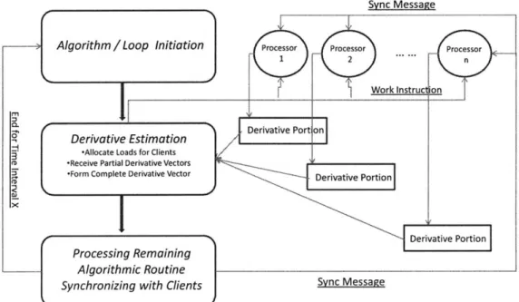
perspective. . . . . 37 4-1 The generic server-client implementation architecture of the Para-EKF
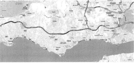
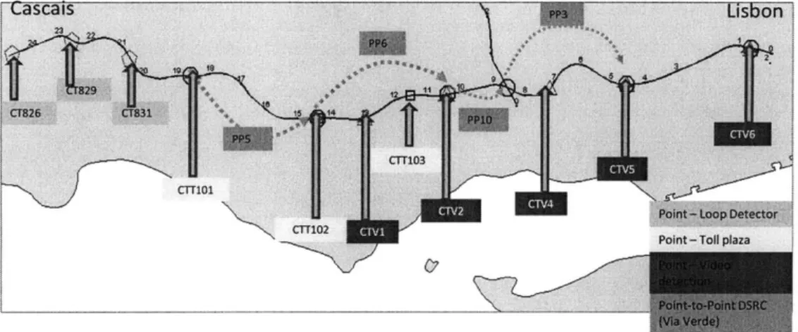
and Para-GD algorithms... . . . . . . . . . . . 74 5-1 The study network - Brisa A5. . . . . 81 5-2 The sensor deployments on the Brisa A5 study network . . . . 82 5-3 A 45 degree plot of estimated sensor counts against observed sensor
counts during off-line calibration. . . . . . . . . 85 5-4 A 45 degree plot of estimated sensor speeds against observed sensor
speeds during off-line calibration . . . . 85 5-5 Comparison of traffic count observations between Dec-10-2009 and
Jan-11-2010 ... .. ... 87 5-6 Comparison of traffic speed observations between Dec-10-2009 and
Jan-11-2010 ... .. ... 88 5-7 Comparison of traffic count RMSN among base-line algorithms . . . . 90 5-8 Comparison of segment speed RMSN among base-line algorithms . . 90
5-9 Comparison of traffic count RMSN among GD, PSP-GD, EKF and PSP-EKF algorithms . . . . 94 5-10 Comparison of segment speed RMSN among GD, PSP-GD, EKF and
PSP-EKF algorithms ... . 94 5-11 Comparison of algorithms' scalability using the average number of
func-tion evaluafunc-tions per state variable per estimafunc-tion interval . . . . 95 5-12 Comparison of algorithms' trade off of scalability against accuracy . . 96 5-13 The speed performance comparison between EKF and GD in their
List of Tables
1.1 Classification of indicative traffic data collection technologies by scope. 21 1.2 Main types of data collected using different sensor type . . . . 22 3.1 Classification of the four base-line candidate algorithms (EKF, GD, CG
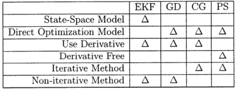
and PS) from framework design, use of derivative and iterative/direct 54 4.1 Distributed Extended Kalman Filter Algorithm - Para-EKF . . . . . 76 4.2 Distributed Gradient Descent Algorithm -Para-GD . . . . 77 5.1 RMSN for the online validation of counts for the four candidate
algo-rithms as well as improvement over the base algorithm . . . . 89 5.2 RMSN for the online validation for speeds for the four candidate
algo-rithms as well as their improvment over the base algorithm . . . . 90 5.3 Algorithm running speed comparison for CG, PS, EKF and GD. . . . 91 5.4 Count RMSN Performance of PSP-GD and PSP-EKF algorithm with
extended state unknowns . . . . 93 5.5 Speed RMSN Performance of PSP-GD and PSP-EKF algorithm with
extended state unknowns . . . . 93 5.6 Computational statistics for distributed implementations of EKF and
GD algorithms. Processor configurations of 2, 3 and 5 are compared. Each is repeated for 5 random seeds . . . . 99
List of Algorithms
The Extended Kalman Filter Algorithm . . . . The Exploration Move Algorithm . . . . The Hooke-Jeeves Pattern Search Algorithm . . . . Non-Linear Conjugate Gradient Algorithm with Polak-Ribiere The Gradient Descent Algorithm . . . . The Bracketing Search Algorithm . . . . The Brent's Parabolic Interpolation Algorithm . . . .
. . . . 51 . . . . 56 . . . . 57 . . . . 58 . . . . 60 . . . . 61 . . . . 62
Chapter 1
Introduction
Contents
1.1 1.2 1.3 1.4 1.5 1.6Thesis Motivation and Problem Statement ... 18
Sensory Technology State-Of-The-Art ... 20
Dynamic Traffic Assignment Framework ... 23
Literature Review ... ... 27
1.4.1 Calibration for off-line applications ... 27
1.4.2 Calibration for on-line applications ... 29
Thesis Contributions . . . . 31
1.1
Thesis Motivation and Problem Statement
Traffic congestion is an important topic in today's society. Not only does it impact the environment, road safety and urban development, it significantly affects the economy. [FHWA, 2001] reported that approximately 30% of daily trips in major US cities occurred within a congested environment in 1997. The economic impact totals $72 billion, which is approximately a 300% increase over 1982. In 2005, travel on U.S. highways amounted to nearly three trillion miles, which is 27.4 billion miles more than in 2004 and almost 25% more than in 1995 [FHWA, 2005].While travel demand expands steadily, road network capacity has remained largely unchanged. Between 1980 and 1999, the total length of highways was only increased by 1.5 percent. The total vehicle-miles travel during the same period increased by 76 percent [FHWA, 2007]. Although the building of new road infrastructure and service networks proves to be an effective way of mitigating congestion, the cost is too high. To that end, much of the present research in transportation science has focused on the better management of existing road capacities.
Intelligent Transportation Systems (ITS) through surveillance systems, commu-nications, and computing technologies, have the potential of facilitating effective management of transportation systems. Centralized among the many research di-rections under ITS is the development of high-fidelity Dynamic Traffic Assignment (DTA) models [Ben-Akiva et al., 1991][Ben-Akiva. et al., 2002]. These simulation-based DTA models are capable of replicating traffic network conditions and provid-ing accurate forecasts as well as travel guidance. They benefit travelers through the avoidance of traffic congestion and the better planning of travel routes and departure time.
One of the key enabling factors for the deployment of such DTA system is the availability of an array of sensors that provides timely, accurate and reliable traffic information. Recent advancements of sensor technologies and their applications in surveillance systems have not only pioneered new methods of collecting and commu-nicating network information, but also revolutionized the way traffic information is
utilized within modern DTA systems for enhanced accuracy and effectiveness. With advancements in technologies, information collected from network sensors can now be gathered in a timely manner for the calibration of DTA systems at their opera-tional time, resulting in significantly improved modeling accuracy and reliability. This process of using available sensory information to adjust DTA models in real-time is known as DTA model on-line calibration.
The topic of DTA on-line calibration using real-time surveillance information has been widely discussed in literature. While accuracy and robustness are important as-pects of DTA on-line calibration, the issue of scalability has received limited attention. For very large networks, the running time of these algorithms is a key determining factor for the successful deployment of these systems. This is because the on-line calibration of DTA systems has much more stringent operational constraints - the calibration procedure has to be completed within limited time intervals. As such, solution approaches that are not scalable for large networks tend to carry little value. While searching for fast candidate algorithms that are applicable for large networks is a top priority, accuracy and robustness cannot be neglected. However, in most cases, as speed improves, accuracy and performance deteriorate. The key is to strike a balance amongst the different objectives, developing accurate, robust and efficient candidate algorithms for the on-line calibration of DTA models.
This thesis explores algorithmic and implementation aspects of the established DTA on-line calibration framework from [Antoniou, 20041. The algorithmic aspect of the on-line calibration entails the exploration of advancements in candidate al-gorithms - all else being equal, how one algorithm outperforms another in terms of accuracy and speed. The answer is not always clear-cut if only one or two methods are addressed. Often an examination of a spectrum of candidates is needed. Apart from algorithmic advancement, this thesis will also address efficient algorithm imple-mentations. Good algorithmic implementations are just as important as the necessity for algorithmic accuracy and effectiveness. For example, a sequential algorithm may have its parallel equivalent implemented, should hardware resources permit. Although identical algorithms are operated, the parallel version of the algorithm may
poten-tially provide faster solutions. The two aspects are essenpoten-tially complementary with each other, and when combined, have the potential to improve the performance of the existing DTA on-line calibration framework.
Before presenting the formulation, two important functional blocks within the DTA on-line calibration framework are first introduced. They are 1) Sensory Data and 2) DTA System.
1.2
Sensory Technology State-Of-The-Art
The important role of sensor technologies in on-line DTA calibration cannot be over-stated. Given the objective of developing fast and effective approaches of on-line calibration algorithms, an abstraction of traffic sensor network that is based on their spatial characteristics and the attributes of the traffic data collected is necessary. In this section, a comprehensive overview of sensor technologies for traffic engineering is provided.
There are currently several technologies for traffic data collection. Each of these technologies has different technical characteristics and principles of operation, includ-ing types of data collected, accuracy of measurements, levels of maturity, feasibil-ity and cost, and network coverage. [Antoniou et al., 2008] categorized sensor types based on functionality as point, point-to-point, and area wide:
Point sensors: This is the most basic type and the most widely used type of sensor used in traffic engineering. Examples of point sensors are inductive loop detectors and loop detector arrays [Oh et al., 2002]. With recent sensor technology advancements, new point sensors such as radar [Nooralahiyan et al., 1998], infrared and point video sensors [Pack et al., 2003] are being developed and deployed.
Point-to-point sensors: Point-to-point sensors can recognize vehicles at multi-ple points in a network. Some point-to-point sensors provide commulti-plete traversal of the travel path while others recognize vehicles at lesser locations. This type of sensor usually provides point-to-point travel time, count, aiding in route choice analysis and OD estimations. Typical sensors in this category are: Automated
Vehicle Identification (AVI) systems [Antoniou et al., 2004], Global Positioning Sys-tem (GPS) [Quiroga et al., 2002], Cell-Phone tracking [Laborczi et al., 2002], License Plate recognition using Dedicated Short Range Communication (DSRC).
Area-wide technologies: These advanced technologies are still under heavy re-search. One example of area-wide traffic sensor is the unmanned helicopter. This helicopter is autonomous and is able to fly from its base to the investigated area. The helicopter can transmit back traffic information in the format of photogrammet-ric, video, sound recording, hazard detection etc. to the Traffic Management Center (TMC) [Srinivasan et al., 2004].
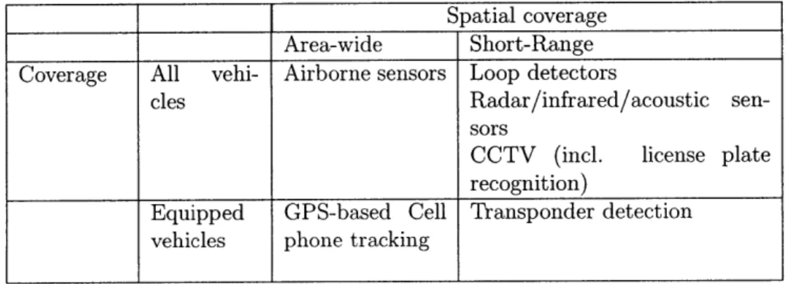
Table 1.1 classifies the various traffic data collection technologies by their spatial and vehicle coverage. Based on their coverage of the network, data collection systems can be organized by whether they can track vehicles throughout the entire network (e.g. GPS systems or cell phone tracking systems) or whether they are limited in identifying vehicles in particular locations of the network (e.g. tag identification sensors, or license plate recognition systems).
Spatial coverage Area-wide Short-Range Coverage All vehi- Airborne sensors Loop detectors
cles Radar/infrared/acoustic
sen-sors
CCTV (incl. license plate recognition)
Equipped GPS-based Cell Transponder detection vehicles phone tracking
Table 1.1: Classification of indicative traffic data collection technologies by scope. Source: [Antoniou et al., 2008]
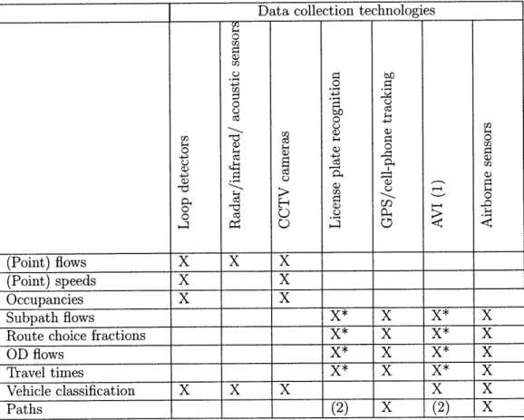
Table 1.2 summarizes the data collection capabilities of each sensor technology. A crucial conclusion, based on these two tables, is that no data collection technol-ogy is clearly superior, instead, their functionalities, in terms of data collected are complementary.
Data collection technologies 0 b0 (Pin) pedsX 0 -OD flws X* X X* 64 0 Paths () X02 o1 Cl) - > ) (Pont flow x x
Rot frciost chic x)
(Oint flows X* X* ______
Travel times X* X X* X
Vehicle classification X X X X X
Paths ____ (2) X (2) X
Table 1.2: Main types of data collected by each sensor type. * Data limited by
network design. (1) This technology could be used to collect practically any type of information collected by the vehicle (including speed profiles, origin, destination, and path). In this table, only the information that can be collected by "dumb" transponders, that simply report a unique vehicle signature, is reported. (2) Possible if a dense network of detectors was available. Source: [Antoniou et al., 2008
1.3
Dynamic Traffic Assignment Framework
Dynamic Traffic Assignment (DTA) [Ben-Akiva. et al., 2002] systems combine so-phisticated driver behavior modeling and traffic network simulation into a unified model. The system comes in two versions: 1) an off-line version of the system is used to evaluate various traffic management strategies such as lane management, incident management, capacity management as well as evacuation and rescue plans; 2) an on-line version of the system is usually used as a short-horizon prediction tool. The applications of the on-line DTA system include but are not limited to: real-time in-cident management, traffic control, emergency vehicle routing and traffic congestion forecasts etc.
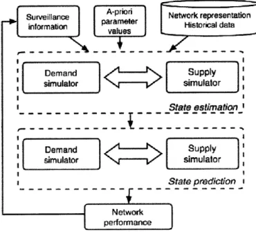
For the purposes of this thesis, the real-time DTA system is of particular interest. The general structure of the model is given in figure 1-1.
Surveillance A-priori Network representation information prameter Historical data
I Ivalues Demand Supply simulator simulator State estimation
Demand
Supply
simulator simulator State prediction Network performanceFigure 1-1: The overall structure of the real-time Dynamic Traffic Assignment sys-tem. It performs state estimation and state prediction. This involves a number of interactions of demand and supply simulation. Source [Antoniou, 2004]
val-ues of the unknown parameters in the DTA model, as well as historical data, such as time dependent OD flow matrices and the network representation. At the core of the system is an iterative process of state estimation and prediction. The purpose of state estimation is to ensure that the internal model's state is consistent with reality. Once state estimation is complete, state prediction is performed. Within state pre-diction, future network conditions are anticipated through Monte-Carlo simulations of drivers' behavior and traffic network. The outputs of the overall system are con-sistent forecasts of network conditions, including link density, flow, speed, as well as travelers' characteristics including their travel time, route choice and departure time. The anticipated information is used to generate guidance and will be incorporated into the next round of calculations [Bottom, 20001.
As can be seen, the most important component of the DTA system is the state estimation and prediction module. This module has two sub-components: 1) Demand simulation and 2) Supply simulation. A detailed description of the interactions of the demand and supply simulator can be found in [Ben-Akiva. et al., 20021.
The traditional approach to demand simulation is to perform real-time Origin-Destination demand estimation and prediction [Ashok and Ben-Akiva, 1993]. OD estimation combines historical and real-time information to obtain the best time-dependent OD matrices. OD prediction uses the current estimation of demand pat-terns and calculates short-term evolution of future demands [Antoniou, 1997].
The supply model is usually a scopic traffic simulator. The choice of meso-scopic simulator is based on the trade-off between simulation detail and model running speed. Meso-scopic simulators allow relatively high resolution of network traffic mod-eling at low cost of computational burden. They consist of the following six major components. 1) Network representation; which represents both static (nodes, links etc.) and dynamic (free flow speed, max and min densities etc.) entities on the net-work. 2) Link output and acceptance capacity model; which simulates movement of vehicles on the boundary between two connecting links/roads. 3) Spill-back model; which models vehicle dynamics during congestion as well as the build up of queues. 4) Speed/density model; which models aggregated vehicle forward speed using road
segment's density information 5) Vehicle movement model; which considers the for-ward movement of vehicles on a link as well as their lateral selections of lanes. 6) Deterministic Queuing model; which models builds up and dissemination of queues, as well as vehicles' delay at intersections.
Figure 1.3 on the next page is a detailed schema of the demand and supply inter-action and information dissemination for DynaMIT, a state-of-the-art DTA system.
Hybrid Demand & Behavioral Simulation LeHistormcal Historical OD population prediced 00disaggregation matrices of drivers ---Updated population of Sre-trip
On-line drivers Behavioral
aggregation (departure time, modes, model route)
Updated OD Latest information
matrices (Network condition,
Driving guidance)
Behavior correction Surveillance (OD estimation (Traffic counts,
And pedicion)Link speed, etc)
Estimated and O-ieActual list of
predicted OD diageaindrivers
matrices
Drivers with En-route
updated 'behavioral
abehaviors model
Meso-Scopic Simulation
Link output
Network and Spill-backs
representation Acceptance capacity model
(Static, Dynamic) model
Vehicle Deterministic
Speed model Movement Queuing
model model
.Monte-Carlo Simulation
Expected Performance
Network characteristicsStaeyBnh rk
(Density, congestion, load)
Notification & Guidance dissemination
(Trael ode)management tme, plan
0 0 0 ct 71 0
ct
0 ze 0d Q c-i -eO1.4
Literature Review
The calibration problem in the domain of DTAs has been widely discussed in the literature of computational transportation science. From the operational point of view, existing literatures on DTA calibration can be grouped into two categories: off-line operation and on-line operation.
This section presents an overview of the calibration methodologies applied to the DTA framework. The first section presents the literature related to DTA off-line cal-ibration with sensory information. The second section focuses on the methodologies for the on-line calibration approaches.
1.4.1
Calibration for off-line applications
[Balakrishna, 2002 studies the problem of off-line calibration using DTA models. In the study, multiple types of sensory data are used to calibrate the DTA model to produce accurate OD estimation and prediction. The objective is to minimize the simulated and observed quantities from the sensor data:
ming3_,,PIIMsi"'
- MobsI1)
where 3 represents the behavior choice parameters, y represents the supply simu-lation parameters and X, are the OD flows departing from time interval p. Mob' are
the sensor observations and M8'm are their corresponding simulated counter-parts. The objective function minimizes the discrepancy between simulated and observed sensory information from various types of sensors. These sensor types include: traffic flows, link speed and densities.
Xh
=
argmirnI Ni (Xh, x N2 (y " , Yh) (The OD estimation is conducted using equation 1.2. Function N1 measures the
discrepancy, in Euclidean distance, between the estimated Xh and their a priori values
xa.
N2measures the discrepancy between the observed vehicle count from loopdetec-tor sensors yA and their simulated counterpart yhm. The calculation of this quantity is: h -m =p (1.3) p=h-p'
where p' is the degree of autoregressive process and ap is an assignment matrix that maps OD flows at time interval h to links on the physical network. A rigorous treatment of assignment matrix can be found in [Ashok and Ben-Akiva, 1993].
The approach is later extended to calibrate both the OD flows as well as travelers' driving behavior parameters [Balakrishna, 2002]. In the study, sensor data are fused within a DTA model to calibrate time dependent OD flow matrices, the variance-covariance error matrix for measurement error, autoregressive parameters as well as driving behavior parameters. An iterative approach that jointly calibrates these parameters is proposed.
[Toledo et al., 2003] conducted off-line calibrations of OD flows and travel behav-ior parameters using microscopic simulations. In the study, aggregated sensor sources are used as inputs. GLS-based OD estimation is conducted to produce explicit con-straints, and bi-level heuristic solution algorithms are used to conduct the overall estimation of OD and behavior parameters.
[van
der Zijpp, 1987] combined volume counts with trajectory information ob-tained from automated license-plate surveys for the estimation of OD flows. A mea-surement equation for the trajectory counts is specified and split probabilities areestimated from combined link volume counts and trajectory counts.
[Balakrishna, 2006] proposed an innovative framework that jointly calibrates both demand simulation (OD flows, behavior parameters) and supply simulation (speed-density relationship, link capacities etc.) DynaMIT, a state-of-the-art DTA system is used to jointly calibrate these parameters in a case study. The study shows promis-ing results in the estimatpromis-ing of unknown parameters from both demand and supply simulation components.
weights, three components:
argmin,3 Ni(M, M) + N2(X, Xa) + N3(, 3a) (1.4)
Where M is the observed sensor observation vector,
M
is their simulated counter-part from DynaMIT with M =f(x,
3). x are the estimated OD flows and Xa is their a priori values.13
is the vector of DTA model parameters including behaviors and supply parameters and#a
is the corresponding vector of their a priori values.N1, N2, NA3 are distance functions with adjustable weights.
The Simultaneous Perturbation and Stochastic Approximation (SPSA) [Spall, 1992] [Spall, 1994b] [Spall, 1994a] [Spall, 1998b] [Spall, 1998a] [Spall, 1999] method is found to be the most promising algorithm.
[Vaze et al., 2009] applied the SPSA method to address the off-line DTA cali-bration problem. In their study, sensor data involving vehicle count and Advanced Vehicle Identification (AVI) information are fused within the DTA framework. The formulation is similar to that of [Balakrishna, 2006]. DynaMIT is used as their can-didate simulation software. The study found that calibration using AVI significantly increased the accuracy of the network traffic prediction.
1.4.2
Calibration for on-line applications
[Ashok and Ben-Akiva, 1993] [Ashok and Ben-Akiva, 2000] formulated the real-time OD estimation and prediction problem as a state-space model and solved it using a Kalman Filtering algorithm. The authors' use of deviations of OD flows from their his-torical values provides an elegant framework for incorporating structural OD informa-tion (generated during off-line calibrainforma-tion) into the on-line process [Antoniou, 1997]. [Ben-Akiva. et al., 2002] implemented this approach in the DynaMIT DTA system.
[Bierlaire and Crittin, 2004] outlined an efficient solution algorithm for the OD estimation problem. The method used is a generalization of the secant method, which uses several past iterations to produce linear approximation of the original non-linear form. The method is very efficient in that it is matrix free and derivative free.
[Antoniou et al., 2004] presented a methodology for the incorporation of AVI infor-mation into the OD estiinfor-mation and prediction framework, which was later extended by [Antoniou et al., 2006] to allow for the consideration of any types of available surveillance data.
[Zhou and Mahamassani, 2006] developed a non-linear ordinary least-squares cal-ibration model to combine and fuse AVI counts, link counts and historical demand information and solved this as an optimization problem.
[Antoniou, 2004] developed an approach that formulates the on-line calibration problem as a state-space model, comprised of transition and measurement equations. A priori values provide direct measurements of the unknown parameters (such as origin-destination flows, segment capacities and traffic dynamics model parameters), while surveillance information (for example, link counts, speeds and densities) is incorporated through indirect measurement equations. The state vector is defined in terms of deviations from the calibration parameters and inputs from available estimates.
[Antoniou et al., 2005] formulated the problem of on-line calibration of the speed-density relationship as a flexible state-space model and presented applicable solution approaches. Three of the solution approaches [Extended Kalman Filter (EKF), Iter-ated EKF, and Unscented Kalman Filter (UKF)] are implemented and applications of the methodology, using freeway sensor data from two networks in Europe and the U.S., are presented. The EKF provides the most straightforward solution to this problem, and achieves considerable improvements in estimation and prediction accu-racy. The benefits obtained from the more computationally expensive Iterated EKF algorithm were shown. Applicable solution algorithms are presented and compared in [Antoniou et al., 2007a].
The most computational burdensome part of the EKF method is the calculation of Jacobian Matrix at each simulation interval. [Antoniou, 2004] further tested the Limiting Kalman Filtering algorithm in the context of on-line model calibration and sensor data fusion. The algorithm is able to achieve comparable performance as that of the EKF during relatively stable network conditions. The idea is to compute an
array of Kalman Gain matrix off-line, and select the most appropriate one. This approach saves a significant amount of computational time.
[Wang and Papageorgiou, 2005] presented a general approach to the real-time es-timation of the complete traffic condition in freeway stretches. They used a stochastic macroscopic traffic flow model together a state-space formulation, which they solved using an Extended Kalman Filter. The formulation allows for the dynamic tracking of time-varying model parameters by including them as state variables to be estimated. Random walk is used as transition equations for the model parameters. A detailed case study of this methodology is presented in [Wang et al., 2007]. The approach is further validated in [Wang et al., 2008], where the joint estimation of supply parame-ters and traffic flow variables is shown to lead to significant advantages: 1) Avoidance of prior model calibration, 2) adaptation of traffic conditions and 3) enabling of inci-dent alarms.
1.5
Thesis Contributions
This thesis makes several concrete contributions to the state-of-the-art, specifically, 1. The feasibility and effectiveness of the on-line calibration framework in a
real-world application using both state-space and direct optimization formulations are demonstrated.
" The framework is tested and successfully verified on a medium network with state variables exceeding 600. Previous on-line calibration studies used state size around 100.
" Multiple sensory technologies are used in the tests, including Via-Verde and automatic Toll Gate Counter technologies. This demonstrates the flexibility of the framework that it does not impose any constraints on the types of sensors that it can handle.
2. A scalable framework design with a single processor: the EKF and PSP-GD algorithms are presented. The algorithms achieve high degree of accuracy
while maintaining low computational complexity.
3. A scalable framework design with multiple processors: Complete C++ imple-mentation of the distributed version of the EKF (Para-EKF) and GD (Para-GD) algorithms within DynaMIT-R. A detailed computational performance analysis is presented along with the Brisa case study.
1.6
Thesis Outline
In the next chapter, we outline the formulations of the on-line calibration problem. The third chapter presents the algorithm selection criteria and illustrates four can-didate algorithms - PS, CG, EKF and GD. Their characteristics and suitability for real-time DTA calibration are also discussed. Chapter four presents practical con-siderations aimed at framework scalability. Efficient variants of the EKF and GD algorithms are presented. In addition, distributed computing techniques are used in implementing the Para-EKF and Para-GD algorithms. Chapter five is a real-world case study that demonstrates the feasibility of the framework. The base-line algorithms and their scalable extensions are compared and analyzed for accuracy, robustness as well as efficiency. Chapter six concludes this thesis and presents brief future perspectives.
Chapter 2
Online Calibration Framework
Overview of Framework. ... 34
2.1.1 In-direct Measurement . . . . 2.1.2 Direct Measurement . . . .
2.1.3 System Inputs and Outputs . . . .
2.2 Problem Formulation . . . . 2.2.1 Notation . . . . . . . ..
2.2.2 Measurement Equations. . . . .. 2.2.3 State-Space Formulation . . . ... 2.2.4 Direct Optimization Formulation . . . .
2.3 Characteristics . . . .
2.3.1 Sensor Type . . . .
2.3.2 Highly Non-linear. . . . . . . .. 2.3.3 Stochasticity... . . . . . . ..
2.3.4 High Cost Function Evaluation . . . . . 2.4 Summary . . . . . . . . 34 . . . . 36 . . . . 36 . . . . 38 . . . . 38 . . . . 38 . . . . 39 . . . . 41 . . . . 42 . . . . 42 . . . . 43 . . . . 43 . . . . 44 . . . . 44
Contents
2.12.1
Overview of Framework
We start by presenting an overview of the general concepts of the on-line calibration framework. The goal is to gather some insights on the intuitions of the methodologies behind the framework. The concept of direct and in-direct measurement is introduced and the inputs and outputs of the on-line calibration framework are summarized.
2.1.1
In-direct Measurement
Sensory information is an important ingredient of the on-line calibration framework
- they inform the model about the observed network conditions. The information provided could include link speed, link density, OD travel time etc. Without loss of generality, the sensory data could come from off-line sources as well as on-line sources. In addition, they need not be from the same types of sensors.
On the other hand, simulation-based DTA models are designed to vividly repro-duce network traffic conditions with high-fidelity. These DTA models are capable of producing their simulated sensory value, such as simulated loop detector counts, simulated link travel time, simulated segment speed, etc. Let Mh" be the sensory observation and Mfhm be the simulated sensory value, the in-direct measurement equation is:
Mos = Msi"' + eos(.1hb h h (2.1)
The DTA models often comprise of a large number of parameters and inputs for adjustment. Depending on the values of these inputs and parameters, they produce predicted network conditions that vary in accuracy. Calibration is used to describe the process of adjusting the model's parameters so that it best reflects reality. In other words, the sensor data described above are used to correct simulated sensory values computed by the DTA simulators. The corrections take place when there are
inconsistencies between the observed sensor values and their simulated counter-parts. Examples of such observed inconsistencies are:
. observed sensor link speed and simulated link speed
* observed sensor point to point travel time and simulated point-to-point travel time
* observed sensor vehicle counts and simulated vehicle counts at specific locations in a network
Such inconsistencies are resulted from a number of errors in the model. Two of the most common types of errors are: 1) Errors between the true model parameters and the existing model parameters, such as true link free flow speeds and the model's existing link free flow speeds. 2) Errors between true model input value and the actual value used, such as the true OD demand level and the actual demand level applied to the model.
In minimizing these errors, we are effectively adjusting the model parameters and OD demand levels so that the simulated sensory information of DTA models can be more consistent with observed real sensory data. Specifically, for each time interval h at operational time, we have:
minrhMhm - Mob"|| (2.2)
where
7r
represents model parameters and the OD flows being calibrated. Mho"b are the sensor observations and Mhm are their corresponding simulated counter-part. The objective function minimizes the discrepancy between simulated and observed sensory information from various types of sensors. These sensor types include: traffic flows, link speed and densities.To construct the correction procedure, DTA models first need to be modified such that each sensor source has its simulated counter-part. This is done by first examining the sensors that are already deployed within a network, and then adding implementations of virtual sensors that are functionally identical to the deployed sensors. For example, if there is a sensor on a network that reports point vehicle counts, a virtual sensor at the corresponding location in the DTA model that reports
point vehicle counts, should be implemented.
2.1.2
Direct Measurement
In addition to in-direct measurement equations that bridge model parameters with observed sensory values, one can easily construct the so-called direct measurement equations, which describe references of the model parameters themselves. For exam-ple, let lr be the model parameters and OD flows at time interval h, all the following
may serve as its direct measurement, which we denote as rg [Ashok, 1996],
7ra = ir" H(2.3) = frh-1 (2.4) h-1 =
S
Feit
(2.5)
p=h-q h-1 =7th+ F(r
7r
(26)
p=h-qThe first and second forms of the a priori are the simplest. They represent the historical and the estimated values from the last time interval, respectively. The third form implies that the model parameters follow an autoregressive process of order q. With M model parameters, FhP is an M by M matrix of effects of irp on 7rh. The fourth
form models the temporal relationship among the deviations in the model parameters by an autoregressive process of order q. The matrix F/ is an M by M matrix of effects
of 7r, -7r, on 7rh - 7rh. It captures correlation over time among deviations which arise
from unobserved factors that are correlated over time. Examples of these factors may include weather conditions, special events, construction or incidents.
2.1.3
System Inputs and Outputs
To summarize, the DTA online calibration framework requires several input
compo-nents. First it needs sensory data. This includes data from different sensors that are
Historical
data
A priori On-line Surveillance parameter calibration data
values
On-line calibrated parameters
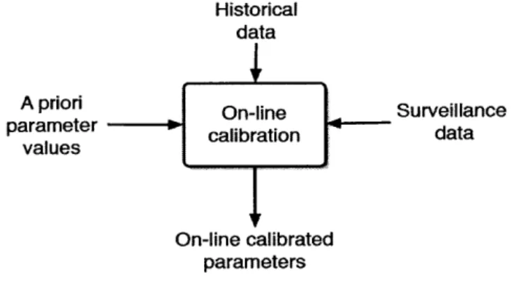
Figure 2-1: The view of the real-time calibration framework from the input/output perspective. Source: [Antoniou, 2004]
DTA model. The model needs to have the corresponding physical sensors imple-mented and be able to generate simulated sensor data. Third, the framework requires a set of a priori parameter values and a priori OD-flow matrices. Finally, the frame-work requires all other necessary information that is needed to operate the model, such as network representations.
The direct outputs of the system are the optimized model parameters (speed-density relationship, route choice, behavior choice etc.) and model inputs (OD de-mand matrices)
1.
These parameters and inputs are highly consistent with sensory observations and thus are used to generate anticipated network forecasts through us-ing the model. In this way, the framework combines low-level sensor data and fuse them into a pool of consistent information for the network. The schema of the on-line calibration framework from the perspective of inputs and outputs is shown at figure 2-1. The framework takes a priori parameter values, historical data on OD flows, and real-time surveillance information and mingles them together using DTA to produce a set of consistent, realistic model parameters. The updated model parameters are then used to generate complete network traffic conditions through simulation.'Existing on-line calibration studies usually include a subset of the model parameters and input variables.
Next, we will specify the core of on-line calibration - how it transforms the inputs and produces outputs. This may be accomplished via a number of approaches. For the purposes of this thesis, two different formulation strategies are presented. We present the classic state-space formulation as well as a direct optimization formulation.
2.2
Problem Formulation
In this section, the on-line calibration problem is formulated mathematically. The state-space formulation is identical to that of [Antoniou, 20041.
2.2.1
Notation
By dividing time period T into time interval 1, 2, 3, ..., N of size t, the network is
represented as a directed graph with a set of links and nodes. Each link is composed of a set of segments. The network contains nL links, nG segments and nOD OD pairs. Furthermore, each segment can be equipped multiple types of sensors. For example, nCount segments are equipped with count sensors and nSeed segments are equipped with speed sensors.
Let 7rh denote the vector of OD flows and model parameters subject to on-line calibration at time interval h. (lrh = {Xh, Yh, Xh is the OD flows at time h and Xh
is the model parameters at time h). Let S denote a DTA simulator and Mh"8 denote a vector of observed traffic conditions for time interval h (For example, travel time, segment flow counts). Let M"' denote a vector of corresponding simulated traffic conditions from S.
2.2.2
Measurement Equations
Two types of information is used: 1) A priori values of the unknown parameter vector are used for the direct measurement and 2) Sensory observations of the network conditions are used for the indirect measurement.
Direct Measurement
The a priori values provide direct measurements of the unknown parameters. The off-line estimates 7,a are commonly used as the a priori estimates.
7rh 7rh + E (.7
Indirect Measurement
The indirect measurement is established through the measurement equation:
Mh m S(rh, 7h-1, ... ,7rh_) = S(Hh) (2.8)
Note that this formulation is flexible and poses no constraint on the types of sensory measurements it can handle. The formulation is general and it assumes that modeled trips can last for longer than one time interval and up to a maximum of p time interval length (Since model parameters for all p intervals may affect the simulated traffic condition). Uh denotes the augmented parameter vector such that
Hh = 7h, rh-1, ..., 7rh_. The relationship between the observed network condition and
their simulated counter-part is:
Mho" = Mhim + ,obs (2.9)
where 6hs can be decomposed into three components: 1) ef 2) e' 3) ie and ebs
Ef
+
6,+
C'. ef captures the structural errors resulting from the inexactness of thesimulation model. d captures the numerical simulation errors, and E' captures the measurement errors. Since it is usually impossible to separate the three components, they are treated together.
2.2.3
State-Space Formulation
The classical approach to model dynamic systems is to use the state-space formu-lation. The state-space model consists of a transition equation and measurement
equations. The first step in defining the state-space formulation is the definition of state. For the on-line calibration of DTA systems, a state consists of model parameters and OD flows. Explicitly, let 7rh denote the state for time interval h, so that:
7Th = [Xh, 7h] (2.10)
The transition equation captures the evolution of the state vector over time. The
general formulation is that: lrh+1 = T(7rh, 7rh-1, -, rh-p) + e+uto, where r is a function
that describes the dependence of 7
h+1 in its previous p states. eat~o is a vector of random errors. In this context, an autoregressive function for T is used. The transition equation is:
h 7
h+1 = Fh+rq + eato (2.11)
q=h-p
The measurement equations are in two parts. The direct measurement equations capture the error between the state vector and its a priori values. That is:
7r" = h ± eh (2.12)
The indirect measurement equation links the state vector with the sensory obser-vations, explicitly, so that:
Mbs = S(7h) + ebs (2.13)
The state-space model is now complete. [Ashok and Ben-Akiva, 1993] proposed to write the state-space model in its deviation form from its historical. The rec-ommendation stems from two main reasons. Firstly, the deviation form implicitly incorporates the wealth of information contained from the offline calibrated param-eters and OD flows. Secondly, the deviation form allows the normality assumption to hold for the error terms in the model. Without using the deviation form the state variables, such as the OD flows, will have a skewed distribution. Normality assump-tion is useful in the applicaassump-tion of Kalman Filtering techniques. For the reasons,
[Ashok
and Ben-Akiva, 1993] and[Antoniou,
2004) write: Arh = 7r - 7rH, and our final state-space model in the deviation form is:A7r =
Air +
eh(2.14)
AM = S(7r/ + Alrh) - M// + e" (2.15)
h
Arh+1 = Fh+l1Ar q e*u* (2.16)
q=h-p
2.2.4
Direct Optimization Formulation
A state-space equivalent formulation is the so-called direct optimization formulation. [Ashok, 1996] discussed the connection between the state-space and the Generalized Least Square (GLS) direct minimization formulations in general, and, Kalman Filter and least square estimation as their respective solutions in specific. It was argued that the application of the results obtained by the classical GLS to discrete stochastic linear processes leads to precisely the Kalman Filter. Therefore an alternative way of formulating the on-line calibration framework is to adopt the GLS direct optimization. In the direct optimization formulation, we jointly minimize the three errors from the
three state-space equations: e', eo"b and eUtu". Because the historicals cancel out
when we subtract each equations for the error terms, the direct optimization can be formulated as:
= argmin[N1(ea) + N2(e0s") + N3(ea"to)] (2.17)
h-1
- argmin[N1(rh - rr) + N2(Mir" - Mhb") + N3(7rh - F +1
wq)] (2.18)
q=h-p-1
If we assume that ea, eobs and e'uto are normally distributed and uncorrelated, and, Ni signifies squared distance, the above can be translated into the following
generalized least square (GLS) formulation: 7r = argmin[(7rh - 7r)'V-1 (7rh - 7h -(M" - M m ) (2.19) h-1 h-1 (rh -
S
F q 1 'Z 1(xh - Fq) q=h-p-1 q=h-p-1Where, V, W and Z are the variance-covariance matrix of ea, eobs and e at re-spectively.
2.3
Characteristics
Before presenting the choice of solution algorithms, this section provides a glance of the key characteristics of the on-line calibration approach 1) The sensory types that it handles, 2) The speed complexity of single evaluations of the loss function, 3) Stochasticity, 4) High non-linearity within the DTA model.
2.3.1
Sensor Type
The formulation of on-line calibration in the state estimation is general and flexi-ble. It does not impose any restrictions on the types of sensors that it can handle. This is one of the primary advantages of simulation-based DTA systems. Equation 2.8 calculates the simulated counter-parts of the corresponding sensor values in the simulated network. The formulation has no requirements on the specifications of the surveillance systems. To construct the correction procedure, DTA models first need to be modified such that each sensor source has its simulated counter-part. This is done by first examining the sensors that are already deployed within a network, and then adding implementations of virtual sensors that are functionally identical to these deployed sensors within the DTA model. These virtual sensors are capable of reporting identical quantities in the simulated network. For example, if there is a sensor on a network that logs point vehicle counts, one shall add an implementation
of a virtual sensor at the corresponding location in the DTA model that reports point vehicle counts.
2.3.2
Highly Non-linear
The second characteristic of the approach is the highly non-linear relationship between the state variables and surveillance information. This can be demonstrated through the speed-density relationship model. The model calculates link speed (A common form of surveillance data) from simulated link density. The following equation is used:
V': = vmax (k
-kmin
) 3)" (2.20)Where the parameters subject to real-time calibration are 1) vmax: the maximal
link speed, 2) kmin: the minimal link density, 3) kjam: the maximal link density at
jam condition, 4) a and /: the segment-specific coefficients.
The inherent non-linearity within the DTA model that the loss function contains complicates the solving of the problem. [Balakrishna, 2006] summarized the compli-cations: 1) The loss function might have several local minimal rather than a unique minima, and searching for the global minima is often very difficult 2) Studying the true shape of the loss function becomes impractical, because of the relationships be-tween observations and the large number of model parameters. 3) The interactions of various models further complicate the feasibility of applications of analytical rep-resentations.
2.3.3
Stochasticity
The DTA system is also stochastic. The system simulates a large set of vehicles and drivers' behaviors. Thus a certain level of stochasticity is necessary to reflect real world decision making. For example, the pre-trip behavior model applies probabilis-tic modeling of driver's choice of departure time and routes. The supply simulator processes vehicles in the network in a certain randomized order at each simulation interval. This helps to replicate real-world network dynamics.
The stochasticity in the underlying DTA model produces noise in the simulated traffic conditions. This might impact the quality of the function and derivative evalu-ations. Empirical analysis has shown small degrees of its affect on simulation perfor-mance. The two most successful calibration algorithms in literature, SPSA for off-line calibration and EKF for on-line calibration, both calculate numerical derivatives in the stochastic setting [Balakrishna, 2006][Antoniou, 2004].
2.3.4
High
Cost
Function Evaluation
Finally, the computational complexity of the DTA simulation model is high - a single evaluation of the loss function entails exactly one running cycle of the DTA simulator for the designated time interval. The running time of the DTA simulation model mainly depends on the driver populations in the model and the network complexity. [Wen, 2009] reported that the overall complexity of the DynaMIT supply simulator for a time interval is O(Q x t), where
Q
is the average number of vehicles in the network and t is the length of the time interval. As the cost of single function evaluation is high, algorithms that perform less evaluations of the loss function are preferred.2.4
Summary
In this section, the DTA model on-line calibration framework is introduced and dis-cussed in detail. The general approach is laid. That is, with the use of a simulation-based DTA system, the framework seeks to minimize 1) The difference between the model parameters and their a priori values and 2) The difference between observed sensory data vector and its simulated counter-part. The inputs of the framework are various surveillance data, a priori time-dependent OD demand as well as a priori model parameters. The outputs of the framework are consistent demand and sup-ply parameter estimates, which the DTA model translates to high-level knowledge of network conditions and traveler benchmarks. The a priori of the OD and model parameters are used to provide direct measurements of the estimates, while the sensor data received in real-time provides in-direct measurements through the DTA model.
The transition equation on the variable state is specified using an autoregressive pro-cess.
The overall approach is mathematically formulated. The state-space formulation models the problem as a dynamic system that evolves over time. It consists of a transition equation, a direct measurement equation and an in-direct measurement equation. Another approach is to formulate the problem as a direct optimization problem. The loss function is composed of the sum of three components corresponding to the three equations in the state-space model: 1) discrepancy between observed and simulated sensor values, 2) discrepancy between model inputs and parameters and their a prior values, 3) discrepancy between model inputs and parameters and their projected estimates from the autoregrssive process. The variables in the scope are time dependent OD levels and appropriate set of model parameters. All elements are constrained within their feasible regions.
With high-fidelity DTA models, the framework is flexible enough to handle various types of surveillance systems. However, complex DTA models are inherently non-linear, making it difficult to come up with a precise image of the loss function. In addition, the solution to the minimization is not unique, since there might be many local minimal. Finally, the level of simulation details dictates longer model running time, making evaluations of the loss function costly.