Precision of Taylor dispersion

(1)

S-1

Supporting Information

Precision of Taylor Dispersion

Patricia Taladriz-Blanco

a

, Barbara Rothen-Rutishauser

a

, Alke Petri-Fink,

a,b

and Sandor Balog

a

*

a_{Adolphe Merkle Institute, University of Fribourg, Chemin des Verdiers 4, 1700 Fribourg, Switzerland} b_{Chemistry Department, University of Fribourg, Chemin du Musée 9, 1700 Fribourg, Switzerland}

ABSTRACT:

*Corresponding author: Sandor Balog (sandor.balog@unifr.ch)

Contents

1. The signal-to-noise ratio of taylorgrams ... 2

2. The uncertainty of determining the width and center of a taylorgram ... 2

3. Taylor dispersion experiments of BSA ... 3

4. Model parameters ... 5

5. The viscosity of water as a function of temperature ... 7

6. Capillary flow temperature by light absorption and heat dissipation ... 7

7. Sampling distributions of normally distributed random variables ... 7

8. Two-window combination of determining the hydrodynamic radius ... 9

(2)

S-2

The signal-to-noise ratio of taylorgrams

It was shown before that the signal-to-noise ratio (𝑆𝑁) of 𝐴, defined as the ratio of the mean and standard deviation of 𝑃(𝐴), is 𝑆𝑁(𝐴) ≅ √𝑁(1 − 𝑇) when 𝑇 > 0.5. 𝑁 = α 𝐼 𝜏 is the number of the photons illuminating the flow during 𝜏 integration time (temporal resolution), 𝛼 a detector-and wavelength-specific constant, and 𝐼 the intensity of the illuminating light.1

This result is obtained via basic principles considering the quantized nature of light and the fundamentals of photon detectors and UV-Vis spectroscopy. To measure the transmission of an analyte and to determine its absorbance, the intensity of the transmitted light is measured. Measuring the intensity of light is never instantaneous, but involves a detection time interval 𝜏 > 0. Detecting photons is intrinsically random, and the consequence is that the number of photons detected during 𝜏 is a random variable. In other words, if one measures the absorbance of a sample 𝑘 times under the very same conditions, one tends to obtain 𝑘 different results. This is because even if the intensity of the illumination is completely stable, the probability density of the photon counts follows a Poisson distribution. This randomness is an inherent property of classical linear spectroscopy and referred to as shot noise. Accord-ingly, measuring transmission (𝑇) and absorbance (𝐴) is also probabilistic, and thus noisy. Due to the relatively fine temporal reso-lution, this stochastic character becomes relevant to Taylor dispersion where a long continuous sequence of short and single meas-urements is required to resolve the dynamics of the band dispersion, while measuring the transmission of the solvent background may be a single and considerably longer measurement. By starting from the Poisson distribution of the photon counts, and by applying the rule of transforming random variables, we calculated the probability density of the absorbance when the intensity of illumination is precisely known and the influence of particle number density fluctuations2_{is negligible: 𝑃(𝐴) = 𝐿𝑛10 ∙ ⅇ}−𝑁∙𝑇_{∙ 𝑁}𝑢_{∙ 𝑇}𝑢_{/𝛤[𝑢] where}

𝑢 = 𝑁 ∙ 10−𝐴_{, 𝑁 = α ∙ 𝐼 ∙ 𝜏 is the number of the photons illuminating the flow during 𝜏 integration time, α a detector-and}

wavelength-specific constant, 𝐼 the intensity of the illuminating light reaching the flow, 𝑇 the value of the transmission, and 𝛤 the gamma function. It can be shown that when 𝑁 > 100, the signal-to-noise ratio (𝑆𝑁) of 𝐴—defined as the ratio of the mean and standard deviation of 𝑃(𝐴)—is

(S1) 𝑆𝑁(𝐴) = −𝐿𝑜𝑔₁₀𝑇 ∙ (𝐿𝑜𝑔₁₀2 + 2) ∙ √𝑇 ∙ 𝑁 .

The mean value of the absorbance is equal to −𝐿𝑜𝑔₁₀𝑇, which is in fact the ‘true’ value one would always measure in the absence of shot noise. When 𝑇 > 0.5, eq 15 simplifies:

(S2) 𝑆𝑁(𝐴) ≅ √𝑁 ∙ (1 − 𝑇).

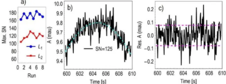
Therefore, the expected value of 𝑆𝑁 is not a constant over the course of a measurement, and it is the highest at the peak of the Taylorgram. The signal-to-noise ratio can be improved by increasing either a) the initial concentration of the sample, b) the capillary diameter, c) the detection area, d) the intensity of the illuminating lamp or by decreasing the temporal resolution. The concentration can be increased as long as a) the Lambert-Beer law remains applicable and b) inter-particle interactions remain negligible. The maximum SN values of the taylorgrams of Figure 1 are shown below.

Figure S1. a) The maximum signal-to-noise ratio of the taylorgrams shown in Figure 1. b) Each SN value was estimated by the best fit of

eq 1 (dashed line) using a ±5s interval around the center of each taylogram. c) The residuals represent noise, and the dashed lines indicate the ±1 standard deviation. The maximum value of the signal-to-noise ratio varies from run to run, and as expected, the absorbance is de-creasing upon dispersion, and thus SN higher for the shorter residence time (𝐿1< 𝐿2).

The uncertainty of determining the width and center of a taylorgram

0.1 𝑠 ≤ 𝜅 ≤ 10 𝑠 300 𝑠 ≤𝑡0≤ 1000 𝑠 0.05 𝑠 ≤ 𝜏 ≤ 1 𝑠 10 ≤ 𝑆𝑁 ≤ 200 0.75 ≤ 𝑇 ≤ 0.95 𝜏 𝜏 𝑃(𝐴) 4 + 1 𝑅2_{> 0.998} 𝜅 𝑡0

(3)

S-3

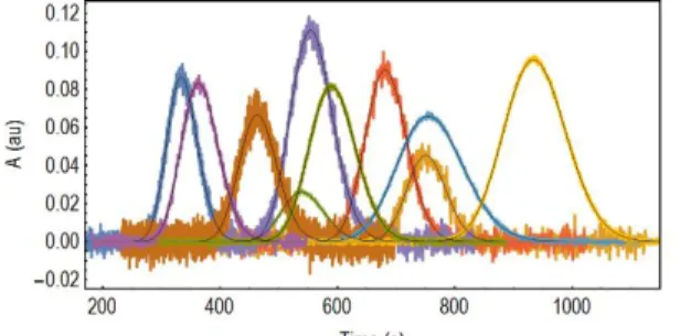
Figure S2. Ten simulated taylorgrams of the 100000 with varying width, center, temporal resolution, noise level, and amplitude. We used

such taylorgrams to determine the expectable precision of measuring 𝜅 and 𝑡0 via fitting eq 1 (black lines).

Figure S3. Predicted and actual precision obtained via simulation experiments. The precision of determining 𝜅 and 𝑡0 agree with a Pearson

correlation coefficient of 0.998 and 0.997, respectively.

Taylor dispersion experiments of BSA

≥ 𝜏

𝑌

𝑃 𝐿

(4)

S-4

(5)

S-5

Model parameters

To fit eq 1 against the experimental data, we used unconstrained nonlinear model fit with three parameters: amplitude, residence time, and width parameter (κ). The taylograms and the corresponding best fits are shown in Figure 1. The tables below also list the coefficient of determination (𝑅2_{) and the maximum signal-to-noise ratio for each taylorgram.}

--- Meas./Window: 1/1 Coefficient of determination: 0.999432 Amplitude: 0.509726 Residence time: 343.999 s Δ(Residence time): 0.00924004 s κ: 1.52675 s Δκ: 0.0019916 s

Max. signal-to-noise ratio: 163 --- Meas./Window: 1/2 Coefficient of determination: 0.999281 Amplitude: 0.500775 Residence time: 629.498 s Δ(Residence time): 0.0127473 s κ: 1.55351 s Δκ: 0.00210706 s

(6)

S-6 Max. signal-to-noise ratio: 179

--- Meas./Window: 4/2 Coefficient of determination: 0.99999 Amplitude: 0.512447 Residence time: 608.022 s Δ(Residence time): 0.0121762 s κ: 1.53822 s Δκ: 0.00202479 s

(7)

S-7 --- Meas./Window: 8/2 Coefficient of determination: 0.999998 Amplitude: 0.506398 Residence time: 604.613 s Δ(Residence time): 0.0116744 s κ: 1.53219 s Δκ: 0.00194041 s

Max. signal-to-noise ratio: 119

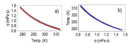
The viscosity of water as a function of temperature

𝑅2_{= 1} _{= 38.41 ± 0.44 10}−6_{Pa s 𝑏 = 432.91 ± 3.02 𝐾}−1_{𝑐 = 160.4 ± 0.46 𝐾}

𝑓−1_{(𝜂) = 𝑐 + 𝑏/𝐿𝑛(𝜂/𝑎)} Capillary flow temperature by light absorption and heat dissipation

We construct a simple a model where the sample temperature is influenced by two phenomena: 1) light absorption generating heat and 2) loss of heat owing to an imperfect insulation of the system from its environment. Given a moderate temperature difference between the capillary flow and its environment (room, housing), the loss of heat can be described by the Fourier law. Furthermore, it is a fair assumption that the temperature of the environment was constant during the measurements, and so were and the parameters describing heat absorption (𝐴) and heat loss (𝑘). According to these assumptions, we construct the following differential equation

(S3) 𝑑𝑇(𝑡)

𝑑𝑡 = 𝐴 − 𝑘(𝑇(𝑡) − 𝑇0)

with the initial condition of 𝑇(0) = 𝑇0.

The solution describes the temperature as a function of time: (S4) 𝑇(𝑡) =𝐴

𝑘(1 − ⅇ −𝑘𝑡_{) + 𝑇}

0.

The total length of a single measurement was nearly 15 minutes, and thus the measurement numbers (1-8) were converted into time accordingly. The two parameters 𝐴[°𝐶ℎ−1_{] and 𝑘[ℎ}−1_{] describe the rate of temperature increase and heat loss. The maximum}

tem-perature this system can reach is 𝐴/𝑘 + 𝑇0.

Figure S5. The temperature as a function of time, and the best unconstrained nonlinear fit of eq S4 (solid gray line). The parameters are

𝐴 = 6.07 °𝐶 ℎ−1_{, 𝑘 = 2.43 ℎ}−1_{, and 𝑇}

0= 24.52 °𝐶. The nominal temperature is indicated by the dashed red line. The dashed gray line

indicates the maximum temperature this system could reach in this series of experiments.

Sampling distributions of normally distributed random variables

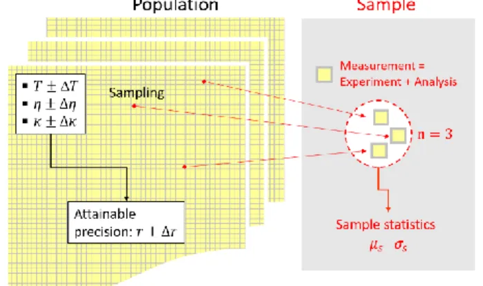
Another important concept relevant to the precision of measurements relates to inferential statistics (Figure S6). From this point of view, each set of individual experiments performed with nominally identical parameters, usually referred to as repeats, represents a random sample drawn from the population. Therefore, the sample statistics, such as the mean and standard deviation vary from sample to sample, and the magnitudes of these variations are functions of the sample size, i.e., the number of repeats. These variations can be described accurately by the sampling distributions of population mean (𝜇) and population standard deviation (𝜎). (Here 𝜇 = 𝑟 and 𝜎 = 𝛥𝑟.) When 𝜇 and 𝜎 describe a normal distribution, the sampling distribution of the measured mean is Gaussian with a mean equal to the population mean, 𝜇_𝑠= 𝜇, and with a standard deviation equal to 𝜎_𝑠= 𝜎/√𝑛. The latter is called as the standard error of the mean, where 𝑛 is the size of the sample. Given that the Gaussian function is symmetric, and the most probable value equals exactly 𝜇, the sample mean is an accurate estimate of the population mean, even if the sample size is small. However, this is not the

(8)

S-8 case for precision. Regarding the sampling distribution of the standard deviation 𝑝(𝜎_𝑠), it is shown by transforming the 𝜒2_{-distribution}

with 𝑛 − 1 degrees of freedom that 𝑝(𝜎𝑠) is generally asymmetric:4

(S5) 𝑝(𝜎_𝑠) =2 3−𝑛 2 ∙ⅇ− 𝑛𝜎𝑠2 2𝜎2∙𝑛 1 2(𝑛−1)∙𝜎1−𝑛_∙𝜎 𝑠𝑛−2 (𝑛−1₂ )

where  is the Euler gamma function. The expected mean and standard deviation (STD) of 𝑝(𝜎_𝑠) are (S6) 〈𝜎𝑠〉 = ∫ 𝜎𝑠 𝑝(𝜎𝑠) 𝑑𝜎𝑠 ∞ 0 = 𝜎√ 2 𝑛 (n/2) (𝑛−1 2 ) and (S7) √〈𝜎_𝑠2_{〉 − 〈𝜎} 𝑠〉2= 𝜎√( 𝑠−1 𝑠 − 2 (n/2)2 𝑠 (𝑛−1₂ )2 )

As shown in Figure S7, sample-to-sample variations have important consequences. First, the expectable measure of precision 〈𝜎𝑠〉

is a function of the sample size. For example, in the case of triplicates one measures three times, and the standard deviation is used as a metric of precision. By calculating the cumulative probability of 𝑝(𝜎𝑠), it is little effort to show that at this sample size the

measure of precision is not reliable at all. When 𝑛 = 3 the probability that 𝜎𝑠< 𝜎 is nearly 78%. In other words, the chance of

underestimating the standard deviation and overestimating the precision is considerable. The chance is 65% when 𝑛 = 10, 57% when 𝑛 = 50, and 55% when 𝑛 = 100. Second, both repeatability and reproducibility are poor when the sample size is not particularly large, because the width of the distribution of 𝜎𝑠 is generally large. For example, when 𝑛 = 3 the width is more than twice as large

as the mean value (Figure S7b).

Figure S6. The view of inferential statistics on measurement analysis. A single measurement consists of an experiment and its analysis. The

population is the ensemble of all the realizable measurements described by the given uncertainties. These parameters ultimately define the attainable precision of measuring the hydrodynamic radius. In contrast to the population, a sample is usually a small set of individual meas-urements (replicates), whose statistics display sample-to-sample variations following the corresponding sampling distributions. These sam-ple-to-sample variations become negligible only when the sample size (𝑛) is large.

Figure S7. Sampling distribution of the standard deviation. a) The probability density of the sample standard deviation at different sample

sizes when the population standard deviation is one. b) The expected sample mean value and sample standard deviation (STD) of 𝑝(𝜎𝑠) as

a function of the sample size.

The sampling distribution of the relative standard deviation as a function of sample size (𝛿_𝑠= 𝜎_𝑠/𝜇_𝑠) was estimated via McKay's approximation.5-7_{The approximation addresses finite-size samples drawn randomly from a normally distributed population, and}

de-fines a variable 𝐾_𝑠 being the following function of the sample statistic: (S8) 𝐾_𝑠(𝛿, 𝑛; 𝛿𝑠) = (1 +

1 𝛿2)

(𝑛−1)𝛿𝑠2

1+𝑛−1_𝑛𝛿𝑠2.

𝛿 and 𝛿𝑠 are the population and sample coefficient of variation, respectively, and 𝑛 is the sample size. McKay showed that when

(9)

S-9 (S9) 𝑓𝑛−1(𝐾𝑠) = { 2 1−𝑛 2 ∙ⅇ−𝐾𝑠2∙𝐾𝑠 𝑛−3 2 ∫ 𝐾𝑠 𝑛−3 2 ⅇ−𝐾𝑠 𝑑𝐾𝑠 ∞ 0 𝐾𝑠> 0 0

To calculate the probability density of the sample coefficient of variation 𝑝(𝛿𝑠), we transform McKay's approximation, and we

obtain the sampling distribution of the relative standard deviation of normally distributed random variables where 𝛿 is the population parameter and 𝑛 is the sample size.

(S10) 𝑝(𝛿𝑠) = 𝑓𝑠−1(𝐾𝑠(𝛿𝑠)) × | 𝜕𝐾𝑠 𝜕𝛿𝑠| (S11) 𝑝(𝛿, 𝑛; 𝛿𝑠) = 2 3 2− 𝑛 2_∙√(𝛿2+1) 2 (𝑛−1)2𝑛4𝛿𝑠2 𝛿4((𝑛−1)𝛿𝑠2+𝑛)4 ∙ ( (1 𝛿2+1)(𝑛−1)𝑛𝛿𝑠 2 (𝑛−1)𝛿𝑠2+𝑛 ) 𝑛−3 2 ∙ ⅇ − (1 𝛿2+1)(𝑛−1)𝑛𝛿𝑠 2 2((𝑛−1)𝛿𝑠2+𝑛) ∫ 𝑥 𝑛−3 2 ⅇ−𝑥_𝑑𝑥 ∞ 0

Two-window combination of determining the hydrodynamic radius

When the hydrodynamic radius is measured via the combination of two windows (S12) 𝑟 =4 𝑘𝐵𝑇

𝜋 𝜂 𝑌2

𝜎22−𝜎12

𝑡2−𝑡1

where 𝜎𝑖2= 𝜅𝑖𝑡𝑖/2, the corresponding relative error is

(S13) 𝛥𝑟 𝑟 = √( 𝛥𝑇 𝑇) 2 + (𝛥𝜂 𝜂) 2 + ℎ2 where (S14) ℎ2₌ 𝑡12 (𝑡1𝜅1−𝑡2𝜅2)2𝛥𝜅1 2₊ 𝑡22 (𝑡1𝜅1−𝑡2𝜅2)2𝛥𝜅2 2₊ 𝑡22(𝜅1−𝜅2)2 (𝑡1−𝑡2)2(𝑡1𝜅1−𝑡2𝜅2)2𝛥𝑡1 2₊ 𝑡12(𝜅1−𝜅2)2 (𝑡1−𝑡2)2(𝑡1𝜅1−𝑡2𝜅2)2𝛥𝑡2 2_.

Impact of noise on numerical integration and temporal moments

By adapting the concept of statistical moments, the temporal moments (mean and variance) are frequently used when characterizing multimodal and polydisperse samples and their optical extinction-weighted average radius.8-10_{In this case, noise affects the attainable}

precision differently than it affects model-based nonlinear regression. To describe this difference, here we outline a straightforward theoretical approach.

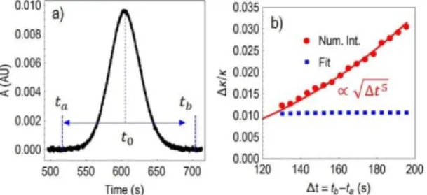
The 𝑛𝑡ℎ_{temporal moment of a taylorgram calculated as a normalized temporal average on the closed interval capped by 𝑡} 𝑎 and 𝑡𝑏

is defined as

(S15) 〈𝑡𝑛_{𝐴(𝑡)〉 =}∫𝑡𝑎𝑡𝑏𝑡𝑛𝐴(𝑡)𝑑𝑡

∫_𝑡𝑎𝑡𝑏𝐴(𝑡)𝑑𝑡

where 𝑡𝑎 and 𝑡𝑏 are chosen that way that they contain the peak of the taylorgram (Figure S8a). Furthermore, 𝑡𝑎 and 𝑡𝑏 are chosen

symmetrically around the center of the peak, i.e. they are at an equal distance from 𝑡0. In experimental practice the taylorgram is not

continuous in time for 𝐴(𝑡) is recorded with discrete timepoints, and thus, the integration becomes a summation, e.g. (S16) ∫ 𝐴(𝑡)_𝑡𝑡𝑏

𝑎 𝑑𝑡 ≅ 𝜏 ∑ 𝐴(𝑡𝑖)

𝑛 𝑖=1

where 𝜏 is the temporal resolution, 𝑡1= 𝑡𝑎 and 𝑡1+ 𝑛 𝜏 = 𝑡𝑏. The temporal mean and temporal variance are

(S17) 𝑀 = 〈𝑡 𝐴〉 = 𝑡0+ 𝜅/2

and

(S18) 𝑉 = 〈(𝑡 − 𝑀)2_{𝐴〉 = 〈𝑡}2_{𝐴〉 − 〈𝑡 𝐴〉}2_{= (𝑡}

0+ 𝜅)𝜅/2.

where from 𝜅 ≅ 2 𝑉/𝑀 when 𝑡₀≫ 𝜅.

In the absence of noise, the precision and accuracy are perfect, and there is neither uncertainty nor bias in determining the value of 𝜅. Accordingly, ∆𝜅 = 0. However, ∆𝜅 does not vanish in the presence of noise. To show this, we consider that the experimentally recorded taylorgram may be decomposed into two terms:

(S19) 𝐴𝜖= 𝐴 + 𝜖

where 𝜖 represents additive noise. The origin of 𝜖 is the shot noise and the related Poisson distribution,1_{and its probability density}

function 𝑝(𝜖) is practically a gaussian. It is easy to show that 𝑝(𝜖) is practically stationary in time, i.e. the variance of 𝑝(𝜖) is basically constant along the taylorgram when the peak absorbance is not too high (i.e. 𝐴 < 0.1). The value of 𝜖 varies randomly along the taylorgram, with a zero mean 𝜖̅ = 0 and variance 𝜖_{̅̅̅ − 𝜖̅}2 2_{= 𝜖}_{̅̅̅. The noise in TDA is also uncorrelated, that is 𝜖}2

𝑖𝜖𝑗

̅̅̅̅̅ = 𝜖_̅̅̅𝛿2

𝑖𝑗, where

𝛿𝑖𝑗 is the Kronecker delta. The overline denotes ensemble average, which is the average over the distribution of the values 𝜖 can take:

(S20) 𝜖̅ = ∫∞ 𝜖 𝑝(𝜖) 𝑑𝜖

−∞

(10)

S-10 (S21) 𝜖̅̅̅ = ∫ 𝜖2 ∞ 2_{𝑝(𝜖) 𝑑𝜖}

−∞ .

Following the definition of the signal-to noise ratio (eq S1), it is easy to show that √𝜖̅̅̅ = 𝐴2

𝑀𝑎𝑥 𝑆𝑁−1≅ 𝐴(𝑡0) 𝑆𝑁−1. The temporal

mean and temporal variance of a noisy taylorgram are calculated the same way as above (S22) 𝑀𝜖= 〈𝑡 𝐴𝜖〉 = 〈𝑡(𝐴 + 𝜖)〉 = 〈𝑡 𝐴〉⏟

𝑀

+ 〈𝑡 𝜖〉 = 𝑀 + 〈𝑡 𝜖〉 (S23) 𝑉𝜖= 〈𝑡2𝐴𝜖〉 − 𝑀𝜖2

and the expected values are calculated via ensemble averring (S24) 𝑀̅̅̅̅ = ∫ 𝑀𝜖 𝜖 𝑝(𝜖) 𝑑𝜖 ∞ −∞ (S25) 𝑉̅ = ∫ 𝑉_𝜖 𝜖 𝑝(𝜖) 𝑑𝜖 ∞ −∞ .

To calculate the expected precision attainable via numerical integration, we need to calculate the ensemble variance of 𝜅𝜖 via the

ensemble variance of 𝑀𝜖 and 𝑉𝜖. These two are practically uncorrelated variables, and thus, we can write

(S26) ∆𝜅2_{= 𝜅} 𝜖2

̅̅̅ − 𝜅̅̅̅𝜖2≅ (2𝑉̅̅̅̅̅̅̅̅̅ 𝑀𝜖)2 ̅̅̅̅̅̅̅ − (2𝑉𝜖−2 ̅̅̅̅)𝜖 2(𝑀̅̅̅̅̅̅)𝜖−1 2

.

We take advantage of the fact that the ensemble variance of the temporal mean is negligible compared to the ensemble variance of the temporal variance, that is, 𝑉_{̅̅̅̅ − 𝑉}_𝜖2

𝜖

̅2≫ 𝑀_{̅̅̅̅ − 𝑀}_𝜖2 𝜖

̅̅̅̅2_{, and thus, we can express the ensemble average as} (S27) ∆𝜅2_≅ (2𝑉̅̅̅̅̅̅̅̅̅̅ −(2𝑉𝜖)2 ̅̅̅)𝜖2

𝑀𝜖

̅̅̅̅2 .

Accordingly, the precision of determining the width parameter is (S28) ∆𝜅 𝜅 ≅ √ 𝑉𝜖2 ̅̅̅̅ 𝑉𝜖 ̅̅̅2− 1.

To evaluate further eq S28, we perform the following steps: (S29) 𝑀_𝜖= 𝑀 + 〈𝑡 𝜖〉

(S30) 𝑉_𝜖= 〈𝑡2_𝐴

𝜖〉 − 𝑀𝜖2= 𝑉 + 〈𝑡⏟ 2𝜖〉 − 〈𝑡 𝜖〉2 𝑉𝑁

= 𝑉 + 𝑉_𝑁 where the term

(S31) 𝑉𝑁= 〈𝑡2𝜖〉 − 〈𝑡 𝜖〉2

may be considered as an analogue of the temporal variance of the noise. It is important to point out, that the temporal noise cannot be treated as a proper probability density function, because it can take negative values as well. Thus, the term is merely an analogy. The ensemble averages are

(S32) 𝑉̅ = 𝑉 + 𝑉𝜖 ̅̅̅ 𝑁 (S33) 𝑉̅𝜖 2 = 𝑉2_{+ 2𝑉𝑉} 𝑁 ̅̅̅ + 𝑉̅̅̅𝑁 2 and (S34) 𝑉̅̅̅̅ = 𝑉𝜖2 2+ 2𝑉𝑉̅̅̅ + 𝑉𝑁 ̅̅̅̅ 𝑁2 thus (S35) ∆𝜅 𝜅 ≅ 𝑉𝜖2 ̅̅̅̅−𝑉̅̅̅𝜖2 𝑉𝜖 ̅̅̅2 = 𝑉𝑁2 ̅̅̅̅−𝑉̅̅̅̅𝑁2 (𝑉+𝑉̅̅̅̅)𝑁2.

Finally, we can write the expression of uncertainty into three distinct groups (S36) 𝑉_{̅̅̅̅ − 𝑉}_𝑁2 𝑁 ̅̅̅2= 〈𝑡̅̅̅̅̅̅̅̅ − (〈𝑡_⏟2_𝜖〉2 ̅̅̅̅̅̅̅)2_𝜖〉 2 1. + 〈𝑡 𝜖〉̅̅̅̅̅̅̅ − (〈𝑡 𝜖〉_⏟4 ̅̅̅̅̅̅̅)2 2 2. − (2〈𝑡_⏟̅̅̅̅̅̅̅̅̅̅̅̅̅̅̅ − 2〈𝑡2_{𝜖〉 ∙ 〈𝑡 𝜖〉}2 ̅̅̅̅̅̅̅ ∙ 〈𝑡 𝜖〉2_𝜖〉 ̅̅̅̅̅̅̅)2 3. where via eq S15 (S37) 〈𝑡̅̅̅̅̅̅̅̅̅ = ∫ (𝑚_𝜖〉𝑛 ∫ 𝑡 𝑚_𝜖 𝑡𝑏 𝑡𝑎 𝑑𝑡 ∫ (𝐴+𝜖)_𝑡𝑎𝑡𝑏 𝑑𝑡) 𝑛 𝑝(𝜖) 𝑑𝜖 ∞ −∞ .

As it can be seen, the precision of determining 𝜅 is a nontrivial function of the noise level and the width of the integration interval. We could not find a straightforward closed-form expression to evaluate eq S37, and therefore, used a numerical approach. Our results indicate that the precision scales as

(S38) ∆𝜅

𝜅 ∝ √ 𝜖 2

̅̅̅ ∙ (𝑡𝑏− 𝑡𝑎)5.

This scaling can be understood by considering that 〈𝑡̅̅̅̅̅̅̅̅̅ = 〈𝑡𝑚_𝜖〉𝑛 ̅̅̅̅̅̅̅̅̅̅̅ = 〈𝑡𝑚∙𝑛_𝜖𝑛_〉 𝑚∙𝑛_{̅̅̅〉 = 𝜖}_𝜖𝑛 _{̅̅̅〈𝑡}𝑛 𝑚∙𝑛_{〉, and 〈𝑡}𝑚∙𝑛_{〉 ∝ 𝑡}𝑚∙𝑛+1_.

Eq S38 means that the precision is improving when the interval of integration becomes shorter, but the precision of numerical integration is inferior to model-based parameter fitting. This is because the uncertainty of model-based parameter fitting is weakly dependent on the interval chosen—provided that the peak is within the interval capped by 𝑡_𝑎 and 𝑡_𝑏—while numerical integration is not. Indeed, when comparing the model-based fit with the temporal moments obtained via numerical integration, the scaling is evident (Figure S8). Finally, it is important to point out that this result is of general validity, and does not depend on the nature of the particle system under study, such as multimodality, polydispersity, and nature of optical extinction.

(11)

S-11

Figure S8. a) A BSA taylorgram and the symmetric interval used for analysis. Being symmetric means that |𝑡0− 𝑡𝑎| = |𝑡0− 𝑡𝑏|. b) The

precision of determining 𝜅 via the temporal moments (Num. Int.) and model-based fitting (Fit). While the latter is practically independent of the interval used, numerical integration exhibits a strong increase with the width of the integral. Accordingly, the integration interval should be kept as narrow as possible.

(12)

S-12

References

(1) Balog, S. Taylor Dispersion of Polydisperse Nanoclusters and Nanoparticles: Modeling, Simulation, and Analysis, Analytical Chemistry, 2018, 90, 4258-4262.

(2) Spears, K. G.; Robinson, T. J. Particle Number Densities by Light-Scattering Fluctuation Analysis, The Journal of Physical Chemistry, 1988, 92, 5302-5305.

(3) Sharma, U.; Gleason, N. J.; Carbeck, J. D. Diffusivity of Solutes Measured in Glass Capillaries Using Taylor's Analysis of Dispersion and a Commercial Ce Instrument, Analytical Chemistry, 2005, 77, 806-813.

(4) Stockburger, D. W. In International Encyclopedia of Statistical Science, Lovric, M., Ed.; Springer Berlin Heidelberg: Berlin, Heidelberg, 2011, pp 1274-1277.

(5) Bossert, D.; Natterodt, J.; Urban, D. A.; Weder, C.; Petri-Fink, A.; Balog, S. Speckle-Visibility Spectroscopy of Depolarized Dynamic Light Scattering, The Journal of Physical Chemistry B, 2017, 121, 7999-8007.

(6) McKay, A. T. Distribution of the Coefficient of Variation and the Extended "T" Distribution, Journal of the Royal Statistical Society, 1932, 95, 695-698.

(7) Forkman, J.; Verrill, S. The Distribution of Mckay's Approximation for the Coefficient of Variation, Statistics & Probability Letters, 2008, 78, 10-14.

(8) Cottet, H.; Martin, M.; Papillaud, A.; Souaïd, E.; Collet, H.; Commeyras, A. Determination of Dendrigraft Poly-L-Lysine Diffusion Coeffi-cients by Taylor Dispersion Analysis, Biomacromolecules, 2007, 8, 3235-3243.

(9) Chamieh, J.; Oukacine, F.; Cottet, H. Taylor Dispersion Analysis with Two Detection Points on a Commercial Capillary Electrophoresis Appa-ratus, J Chromatogr A, 2012, 1235, 174-177.

(10) Balog, S.; Urban, D. A.; Milosevic, A. M.; Crippa, F.; Rothen-Rutishauser, B.; Petri-Fink, A. Taylor Dispersion of Nanoparticles, Journal of Nanoparticle Research, 2017, 19, 287.