Publisher’s version / Version de l'éditeur:
Pair Programming Illuminated, Addison Wesley, 2002, 2002
READ THESE TERMS AND CONDITIONS CAREFULLY BEFORE USING THIS WEBSITE. https://nrc-publications.canada.ca/eng/copyright
Vous avez des questions? Nous pouvons vous aider. Pour communiquer directement avec un auteur, consultez la première page de la revue dans laquelle son article a été publié afin de trouver ses coordonnées. Si vous n’arrivez pas à les repérer, communiquez avec nous à [email protected].
Questions? Contact the NRC Publications Archive team at
[email protected]. If you wish to email the authors directly, please see the first page of the publication for their contact information.
Archives des publications du CNRC
This publication could be one of several versions: author’s original, accepted manuscript or the publisher’s version. / La version de cette publication peut être l’une des suivantes : la version prépublication de l’auteur, la version acceptée du manuscrit ou la version de l’éditeur.
Access and use of this website and the material on it are subject to the Terms and Conditions set forth at
An Economic Analysis of Pair Programming
Erdogmus, Hakan; Williams, L.
https://publications-cnrc.canada.ca/fra/droits
L’accès à ce site Web et l’utilisation de son contenu sont assujettis aux conditions présentées dans le site LISEZ CES CONDITIONS ATTENTIVEMENT AVANT D’UTILISER CE SITE WEB.
NRC Publications Record / Notice d'Archives des publications de CNRC:
https://nrc-publications.canada.ca/eng/view/object/?id=1dc2e6d5-6697-4c01-9873-2cdbf936ea21 https://publications-cnrc.canada.ca/fra/voir/objet/?id=1dc2e6d5-6697-4c01-9873-2cdbf936ea21Institute for
Information Technology
Institut de technologie de l’information
An Economic Analysis of Pair Programming *
Erdogmus, H., and Williams, L.
2002
* published in: Laurie Williams and Robert Kessler, "Pair Programming Illuminated", Addison Wesley, 2002, pp 221-236. NRC 44961.
Copyright 2002 by
National Research Council of Canada
Permission is granted to quote short excerpts and to reproduce figures and tables from this report, provided that the source of such material is fully acknowledged.
Appendix B
An Economic Analysis of Pair
Programming
by Hakan Erdogmus and Laurie Williams
In this appendix, we present a detailed economic analysis of pair programming based on the empirical study conducted at the University of Utah, as discussed in Chapter 4. (You should probably read Chapter 4 before reading this because we won’t go back over the details of the experiment.) In Chapter 4, we indicated that pairs produce higher quality code but that it might take 15% longer to produce this higher quality code. Once code is written, it then goes on to testing and ultimately to the customer. When you consider the savings of putting higher quality code into test and into the hands of the customer, our economic analysis shows that this initial 15% cost is more than made up for. We write this appendix for the reader who would like to know more about how we can claim the overall lifecycle affordability of pair programming.
Introduction
The economic feasibility of pair programming is a key issue. Many instinctively reject pair programming because they think that code development costs will double. If it is more expensive, managers simply will not permit it. Naturally, the goal of a software firm is to be as profitable as possible while providing their customers with the best, high-quality products quickly and cheaply. Organizations decide whether to adopt process improvements based on the business value of their outcome.
First, we compute and analyze a basic comparison of the processes. This basic comparison indicates that pairs perform better considering efficiency and overall productivity. We further this basic comparison by incorporating additional factors into a more complex Net Present Value (NPV) analysis. This economic comparison indicates that pair programming should be considered as an economical alternative over solo programming. NPV considers the time-value of money: the premise that a dollar today is worth more than a dollar in the future. Economic models based on NPV have previously been suggested to evaluate the return on software quality and infrastructure initiative (Boehm 1981, Erdogmus 1999, Erdogmus and Vendergraaf 1999, Favaro et al. 1998, Levy 1987).
Factors of the Basic Comparison Model
Sound research design guides us to have only one experimental variable, the variable under study. Programmers create software using a variety of software development practices. We ensured all
programmers in the study used all the same practices (for design, testing, etc.) except for the experimental variable, the work unit: solo programmer versus pair of programmers working in tandem. In our analysis, we refer to the work unit as:
• N: size of the work unit (persons). The number of developers in a work unit. N equals 1 for a solo programmer (hereby, a soloist), and 2 for a pair of programmers (hereby, a pair). The values of the several model variables we use are determined based on past research studies and statistics reported in the literature. The chosen values are primarily for illustration purposes. The actual values could be different, and they would most likely be both project- and skill-dependent. However, we believe the general conclusions we make are still sound with reasonable variability of these values.
• π. new-code productivity (LOC/person-hour). The average per-person hourly output (LOC) of new code for the work unit.
According to a study by Hayes and Over (Hayes and Over 1997), the average productivity rate of 196 developers who took PSP training was 25 LOC/hour. This figure will be the chosen value of π for N = 1 (soloist).
Anectodal evidence (Wiki 1999, Auer and Miller 2001) suggests that pairing does not take any additional time over solo programming. However, the University of Utah experiment indicated that pairs might take 15% more time than solo programmers. In our analysis, we are conservative and assume that the observed 15% difference is real (despite the fact that, statistically speaking, this difference was insignificant). With this assumption, in a single person-hour, each developer of a pair produces an average of 25/(1.15) = 22 LOC. Thus, for
N = 1 we use π = 25 LOC/person-hour, and for N = 2, π is taken to be a conservative 22
LOC/person-hour.
• β. defect rate (defects/LOC). The average number of defects per unit of output (LOC) associated with the work unit.
According to Jones (Jones 1997), code produced in the US has an average of 39 raw defects per KLOC. This statistic is based on data collected from such companies as AT&T, Hewlett Packard, IBM, Microsoft, Motorola, and Raytheon,with formal defect tracking and
measurement capabilities. According to the same reference, on average, 85% of all raw defects are removed via the development process, and 15% escape to the client. Together the two pieces of statistics suggest an average defect rate of (39)(0.15) = 6 defects/KLOC. This figure represents defects that escape to the customer. The number is consistent, though on the low side, with data from the Pentagon and the Software
Engineering Institute, which indicate that typical software applications contain 5-15 defects per KLOC (Gross et al. 1999). We adopt the average 6 defects/KLOC (or .006 defects/LOC) as the value of β for N = 1 (soloist).
As was discussed in Chapter 4, the code written by the pairs in the experiment passed an average of 90% of the specified acceptance tests compared to code written by soloists, which passed on average only 75% of the same test suite. This result suggests that pairs have only 40% of the defects that solo programmers have after acceptance tests. If we assume that this ratio is retained in defects that escape to the customer, we can adopt as the value of β for N = 2 (pair) is (6)(0.4) = 2.4 defects/KLOC.
• ρ. rework speed (defects/person-hour). The speed at which defects are fixed by the work unit following the deployment of a piece of code.
A study of a set of industrial software projects from a large telecommunications company (Russel 1991) showed that each defect found by a customer required an average of 4.5 person-days, or 33 person-hours of subsequent maintenance effort or rework (based on a 7.5-hour workday). This statistic is consistent with data reported by Humphrey (Humphrey
1995). Based on this observation, the rework speed ρ for N =1 (soloist) is taken to be 1/33 = 0.03 defects/person-hour.
No data is available regarding the effect of pair development on rework activities. We will assume pairs will perform rework with the same 15% cost relative to soloists as was found in the experiment. Under this assumption, the estimated rework speed ρ for N = 2 will be 0.03/1.15 = 0.026 defects/person-hour.
The Basic Comparison Model
In the basic comparison model, we compare three metrics, ε (efficiency), π (new-code productivity), and π0
(overall productivity).
Efficiency
Efficiency is defined as the percentage effort spent on developing new code relative to the total lifecycle
effort (which includes the effort expended on rework).
Given a productivity rate of π, the effort required in person-hours to deploy ω lines of code of output is given by:
:= Epre ωπ
This quantity specifies the initial development (or pre-deployment) effort, and is followed by rework (or
post-deployment) effort once the code has been delivered to the client.
Rework effort, Epost, is the maintenance effort expended due to runaway defects after a piece of new code has been deployed.
:= Epost ω β
ρ
Here ωβ is the number of defects and ρ is the speed of rework. Effort is always adjusted to the work unit by multiplying it by the work unit size N.
Total effort, Etot, is the sum of the initial development and rework efforts: :=
Etot ω (ρ β ππ ρ + )
Efficiency, ε, is then the ratio of the initial development effort Epre to the total effort Etot. It is given by: =
ε ρ β π + ρ The percentage effort spent on rework then equals 1 – ε, or:
β π + ρ β π
Overall Productivity
Overall productivity, π0, is the average hourly output of defect-free code per programmer hour (assuming
that the code is defect-free after rework). It equals the total output ω in LOC divided by the total effort Etot in person-hours. This measure shows just how much the “realized productivity” can be dominated by the extensive cost of rework late in the lifecycle. Expressed in terms of efficiency and new-code productivity, overall productivity is given by:
:= π0 π ε
Results
Table 1 compares a soloist to a pair with respect to the metrics efficiency, new-code productivity, and
overall productivity. In each row, the cell in bold typeface indicates the more favorable alternative with
respect to the corresponding metric. Pairs fair considerably better in efficiency and overall productivity, indicating that initial investments in quality during pair programming pays for itself over the product lifecycle.
Table 1. Comparison of a soloist to a pair. Soloist Pair Efficiency (ε) (decimal %) .17 .34 New-code productivity (π) (LOC/person-hour) 25 22 Overall productivity (π0) (LOC/person-hour) 4.3 7.4
Factors of the Economic Comparison Model
The second comparison model is more complex than the basic comparison model and considers additional important factors that determine economic feasibility.
A software project incurs costs as it accumulates labor hours and realizes value as it delivers functionality. A project is economically feasible when the total value it creates exceeds the total cost it incurs. We assume that the net value generated depends on (1) the project’s labor cost, (2) the time value of money/present value, and (3) the value that the project earns proportionate with the output it produces. The following sections discuss the factors and the underlying parameters that will be used in the advanced analysis.
Labor Cost
Programmer labor (C) is often the most important cost driver in a software development project. We will assume that initial development and rework are performed by the same work unit, resulting in the same constant value for both variables. Since C is assumed to be invariant, we will later be able to eliminate it using a ratio metric.
Time Value of Money and Present Value
When costs and benefits of a project are spread over time, the time at which the costs are incurred and benefits are realized must be taken into account. A cash flow expected to occur in the future is worth less in today’s dollars than a cash flow that occurs now. As the time horizon widens, the difference between the value of a dollar today and the value of a dollar in the future also widens. Time value of money captures the spread between these two values. . Discounting is the process of downward adjusting a future cash flow to express it in today’s value using a compound interest rate, called the discount rate. The discounted value of the cash flow is referred to as the present value (PV).
In economic terms, cost and benefits of a project are represented as negative and positive cash flows, respectively, that occur at specific points in time. The fundamental implication of time value of money is that a project should earn as fast as possible and spend as slow as possible to generate maximum economic benefit.
Earned Value
Earned value (EV) expresses the output produced by a work unit using a linear relationship between development effort and value. Each unit of new code produced earns a fixed amount of value. We assume that rework effort does not earn any value. Only projects that are 100% efficient earn extra value for each labor hour, creating a disincentive to produce defective code, and conversely, an incentive to produce quality code.
Let unit value, V, refer to the average value earned by one unit of output produced. In our case, V is the average value of a single line of new code. Then, earned value corresponding to an output of ω lines of code is given by:
:= EV Vω
Value Realization
Realized value is value that is realized by the client when a functional, defect-free product has been
delivered to a customer. Earned value is not the same as realized value. For example, earned value may never be realized if a project fails to deliver a functional product to the client.
The Software Factory Model
For our economic analysis, we consider a value realization model called the Software Factory. New code is developed, deployed, and reworked in very small increments. Initial development of new code and rework of deployed code are intertwined in a never-ending cycle. Value is realized in very small increments as micro-chunks of new functionality are gradually delivered. Consequently, earned and realized value are essentially the same. The Software Factory model is illustrated in Figure 2. The ticks represent micro-deployment points where small chunks of new code are delivered incrementally. In the perfect (idealized) version of the Software Factory model, the distance between two deployment points approaches to zero, resulting to a truly continuous process. Emerging agile software development methodologies (Fowler 2000) such as XP (Beck et al. 2001) and SCRUM (Rising 2000) support frequent delivery of working code to customers. Agile methodologies are best treaded under the Software Factory.
Start
Rework
…
Deploy Deploy Deploy Deploy Deploy
Rework Rework ReworkRework
Defect Recovery Efficiency
Defect recovery efficiency involves two components: latency and coverage. Latency is the elapsed time between the deployment of a software artifact and the discovery of a fault by the client. Coverage is the number of defects reported or discovered in relation to the total number of defects (including those that have not been discovered). In practice, the discovery of defects by the client can neither be instantaneous nor complete. For example, Jones (Jones 1997) states that in large industrial projects, more than half of the defects in customer code have a latency of one year, while total coverage four years after deployment hovers around 97%.
In emerging, agile processes, the continuous testing and frequent client feedback are believed to lead to a defect recovery with low latency and high coverage. In our analysis, we assume a perfectly efficient defect recovery process: one with full coverage and zero latency. These idealized conditions are opposing in terms of their impact on net value generated: while increased coverage tends to decrease net value, increased latency tends to increase it. When time value of money is taken into account, these assumptions lead to a conservative overall bias, with a mild tendency to underestimate net value. However the level of underestimation may be different for different development processes.
The Economic Comparison Model
Net Present Value (NPV)
Capital investment decisions are often made based on the concept of Net Present Value (Ross 1996). Economic models based on NPV have previously been used to evaluate the return on software quality and infrastructure initiatives (Levy 1987, Boehm 1981, Erdogmus and Vandergraaf 1999, Favaro et al. 1998).
NPV is the difference between the present value of benefits and the present value of costs: NPV = PV(benefits) – PV(costs),
where PV denotes present value.
A project is thought to have business value when its Net Present Value, NPV, is positive, and to be unprofitable when its NPV is negative. Among a set of possible projects, the one with the highest NPV generates the most value, and should be favored over the others.
For the Software Factory model, NPV reduces to: :=
NPV∞ IRV − TDC∞
Here IRV denotes Incremental Realized Value and TDC denotes Total Discounted Cost. Each of these will be discussed below.
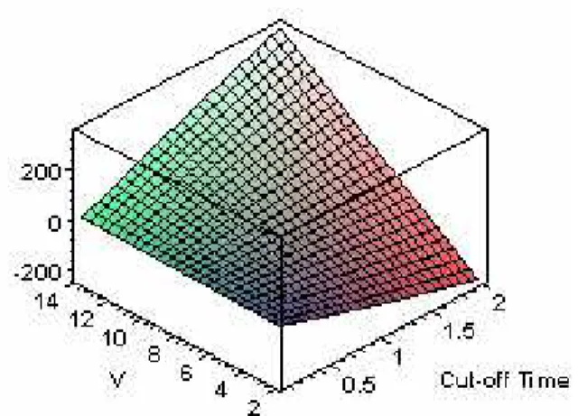
NPV is very sensitive to changes in V, the average value earned by one unit of output produced, measured
in $/LOC. Figure 3 shows how NPV varies as V and time horizon of the project increases for a pair under the Software Factory model, where the labor cost C is fixed at $50/hour. Note that the slope of the NPV curve changes drastically along the output axis as V varies.
Due to this sensitivity, our interest is not on NPV per se. We need a derived metric whose value can be used to rank two alternatives independent of a particular choice of unit value and of the constant labor cost C. Breakeven Unit Value meets the first need.
Figure 2: NPV for a pair under the Software Factory model as a function of unit value V and
cut-off time τ for a fixed annual discount rate of δ = 0.1. Output is plotted in KLOCs. Cut-off time,
measured in years, represents the time horizon of the project. Labor cost is fixed at C = $50/hour.
Breakeven Unit Value
Breakeven Unit Value (BUV) is the threshold value of V above which the NPV is positive. BUV is
determined by solving the equation NPV = 0 for V. Recall that V is measured in $/LOC, based on the assumption that each unit of output produced increases the value earned by a constant amount. A small BUV is better than a large BUV. As BUV increases, a project becomes less and less worthwhile, because higher and higher margins are required to turn a profit. In the Software Factory model, BUV also makes the economic comparison independent of the particular choice of the discount rate.
BUV in the Software Factory
When both value realization and cost accumulation are continuous and incremental, BUV’s dependence on both output and discount rate is broken. However, BUV remains dependent on C, the hourly labor late. For example, for a fixed labor cost of C = $50/person-hour, a soloist achieves a BUV of $12/LOC while a pair a BUV of $7/LOC, indicating an advantage for the pair. These are the minimum marginal benefits required in the Software Factory for a project to break even.
Breakeven Unit Value Ratio (BUVR)
A comparison can be made between the return on investment offered by two different processes through an examination of the ratio of their BUVs.
Define BUV Ratio (BUVR) as the ratio of the BUV of a soloist to the BUV a pair. =
BUVR BUVsolo BUVpair
Values of BUVR greater than unity indicate an advantage for pairs; values smaller than unity indicate an advantage for soloists. As this ratio increases, the advantage of the pair over the soloist also increases.
The metric BUVR makes the comparison between the two work units not only independent of V, but also of the hourly labor cost C.
BUV Ratio in the Software Factory
The BUV Ratio, BUVR, under the Software Factory model is given by: =
BUVR∞
πpairεpair π
soloεsolo
Taking the ratio effectively eliminates the invariant C that appears in the BUV equation. The value of
BUVR is thus constant at 1.7 representing roughly a 40% advantage for the pairs over the soloist. Note
that this advantage is independent of time value of money (discount rate), output produced, cut-off time (time horizon of the project), and labor cost. Effectively, we obtain a metric that provides an all-round comparison.
Derivation of BUV Ratio
For those mathematically-inclined readers, we now derive the BUV ratio. Otherwise, skip right to the summary at the end.
Marginal Value Earned
We need to consider Marginal Value Earned (MVE) in order to calculate Incrementally Realized Value (IRV), the first component in the NPV formula for the Software Factory. MVE is the average value earned per additional unit of elapsed time (measured in $/year; elapsed time refers to compressed time). Given a completion or cut-off time of τ, MVE equals:
:= MVE EV =
τ Vω
τ
Representing output ω in terms of elapsed time eliminates the variable τ, allowing MVE to be expressed in terms of productivity π and efficiency ε. Let the constant hy denote the total number of labor hours in a calendar year. Then MVE can be rewritten as:
:=
MVE Vπ ε hyN
Incrementally Realized Value
Incrementally Realized Value (IRV) is the total value earned within a given time period. Value realized is
discounted as earned. If τ is the time to project completion or the cut-off time, then IRV is given by: := IRV ⌠ d ⌡ 0 τ MVE e(−δ t) t
Here δ denotes the continuously compounded annual discount rate. (Using continuous compounding, the present value of a future cash flow X that occurs in t years is given by Xe–δt.) Expressed in terms of efficiency ε and productivity π, IRV equals:
:= IRV −V π ε h yN (e − ) (−δ τ) 1 δ Marginal Cost
Marginal Cost (mC∞) is the expected incremental cost of initial development and rework per additional unit of elapsed time. Since in the Software Factory model, initial development and rework are intertwined, marginal cost can be written as:
:= mC∞
+
Eε Cpre E (1 − ε C) post τ
where E is the total effort. When pre- and post-deployment costs are equal (i.e., Cpost = Cpre = C), marginal cost is simply:
= mC∞ hyN C
Total Discounted Cost
In the Software Factory, labor costs are discounted as they are incurred to calculate the Total Discounted
Cost, the second component of the NPV formula:
:= TDC∞ ⌠ d ⌡ 0 τ mC∞e(−δ t) t
After substituting the marginal cost with the corresponding term, the above definite integral reduces to:
:= TDC∞ −
hyN C (e(−δ τ) − 1) δ
BUV in the Software Factory
BUV under the Software Factory model is obtained by solving the equation NPV∞ = IRV – TDC∞ = 0 for
the unknown V. This yields:
:= BUV∞ π εC
The formula for the BUV Ratio immediately follows from the above expression.
Summary
The results of our analyses demonstrate the potential of pair programming as an economically viable alternative to individual programming. Using the empirical results that demonstrated that pairs produce higher quality code in 15% more time that individuals, we showed that pairs have a higher efficiency and overall productivity rate. Additionally, considering a more complex economic model, which considered Net Present Value, we demonstrated that pairs increase the business value of a project by significantly reducing the minimum marginal benefit required for a project to break even.
References:
Auer, K. and Miller, R. (2001), XP Applied. Reading, Massachusetts: Addison Wesley.
Basili, V. R., F. Shull, and F. Lanubile (1999), “Building Knowledge Through Families of Experiments,” IEEE Transactions on
Software Engineering, vol. 25, pp. 456 - 473.
Beck, K. (2000), Extreme Programming Explained: Embrace Change. Reading, Massachusetts: Addison-Wesley. Beck, K. and Fowler, M. (2001), Planning Extreme Programming. Reading, Massachusetts: Addison Wesley.
Beck, K., M. Beedle, A. v. Bennekum, A. Cockburn, W. Cunningham, M. Fowler, J. Grenning, J. Highsmith, A. Hunt, R. Jeffries, J. Kern, B. Marick, R. C. Martin, S. Mellor, K. Schwaber, J. Sutherland, and D. Thomas (2001), “The Agile Manifesto,” , http://www.agileAlliance.org
Beck, K. and D. Cleal, “Optional Scope Contracts,” White Paper, Three Rivers Institute, 1999. http://www.xprogramming.com/xpublications.htm.
Boehm, B. W. (1981), Software Engineering Economics. Englewood Cliffs, NJ: Prentice-Hall, Inc.
Cockburn, A. and Williams, L. (2000), “The Costs and Benefits of Pair Programming,” presented at eXtreme Programming and Flexible Processes in Software Engineering -- XP2000, Cagliari, Sardinia, Italy.
Cockburn, A. and Williams, L. (2001), “The Costs and Benefits of Pair Programming,” in Extreme Programming Examined, G. Succi and M. Marchesi, Eds. Boston, MA: Addison Wesley, pp. 223-248.
Constantine, LL. (1995), Constantine on Peopleware. Englewood Cliffs, NJ: Yourdon Press.
Coplien, J. O. (1995), “A Development Process Generative Pattern Language,” in Pattern Languages of Program Design, James O. Coplien and Douglas C. Schmidt, Ed. Reading, MA: Addison-Wesley, pp. 183-237.
Erdogmus, H. (1999), “Comparative evaluation of software development strategies based on Net Present Value,” presented at International Conference on Software Engineering Workshop on Economics-Driven Software Engineering, California. Erdogmus, H. and J. Vandergraaf (1999), “Quantitative Approaches for Assessing the Value of COTS-centric Development,”
presented at Sixth International Symposium on Software Metrics, Boca Raton, FL.
Favaro, J. M., K. R. Favaro, and P. F. Favaro (1998), “Value-Based Software Reuse Investment,” Annals of Software
Engineering, vol. 5, pp. 5-52.
Fowler, M. (2000), “Put Your Process on a Diet,” in Software Development, vol. 8, 2000, pp. 32-36. Gross, N., M. Stepanek, O. Port, and J. Carey (1999(, “Software Hell,” in Business Week, 1999, pp. 104-118.
Hayes, W. and J. W. Over (1997), “The Personal Software Process: An Empirical Study of the Impact of PSP on Individual Engineers,” Software Engineering Institute, Pittsburgh, PA CMU/SEI-97-TR-001, December 1997.
Jones, C. (1997), Software Quality: Analysis and Guidelines for Success. Boston, MA: International Thomson Computer Press. Humphrey, W. S. (1995), A Discipline for Software Engineering. Reading, Massachusetts: Addison Wesley Longman, Inc. Leby, L. S. (1987), Taming the Tiger: Software Engineering and Software Economics. New York: Springer-Verlag, 1987. Nosek, J. T. (1998), “The Case for Collaborative Programming,” in Communications of the ACM, vol. March 1998, pp. 105-108. Rising, L. and N. S. Janoff (2000), “The Scrum Software Development Process for Small Teams,” IEEE Software, vol. 17. Ross, S. A. (1999), Fundamentals of Corporate Finance: Irwin/McGraw-Hill, 1996.
Russell, G. W. (1991), “Experience with Inspection in Ultralarge-Scale Developments,” IEEE Software, vol. January 1991, pp. 25-31.
Succi, G. and Marchesi (2001), M., Extreme Programming Examined. Boston: Addison Wesley. Wake, W. C. (2001), Extreme Programming Explored. Boston: Addison Wesley.
Wiki (1999), “Programming In Pairs,” in Portland Pattern Repository, accessed June 29, 1999, http://c2.com/cgi/wiki?ProgrammingInPairs.
Williams, L. A. (2000), “The Collaborative Software Process PhD Dissertation,” in Department of Computer Science. Salt Lake City, UT: University of Utah.
Williams, L., R. Kessler, W. Cunningham, and R. Jeffries (2000), “Strengthening the Case for Pair-Programming,” in IEEE
Software, vol. 17, pp. 19-25.
Williams, L. A. and R. R. Kessler (2000), “All I Ever Needed to Know About Pair Programming I Learned in Kindergarten,” in