en fr

(1)

HAL Id: tel-01690749

https://tel.archives-ouvertes.fr/tel-01690749

Submitted on 23 Jan 2018

HAL is a multi-disciplinary open access archive for the deposit and dissemination of sci-entific research documents, whether they are pub-lished or not. The documents may come from teaching and research institutions in France or abroad, or from public or private research centers.

L’archive ouverte pluridisciplinaire HAL, est destinée au dépôt et à la diffusion de documents scientifiques de niveau recherche, publiés ou non, émanant des établissements d’enseignement et de recherche français ou étrangers, des laboratoires publics ou privés.

Fatima Herranz-Trillo

To cite this version:

Fatima Herranz-Trillo. Disentangling structural complexity in proteins by decomposing SAXS data with chemometric approaches. Human health and pathology. Université Montpellier, 2017. English. �NNT : 2017MONTT044�. �tel-01690749�

(2)

(3)

(4)

Abstract

Many biological systems are inherently polydisperse, presenting multiple coexisting species differing in size, shape or conformation (i.e. oligomeric mixtures, weakly bound complexes, and species appearing along amyloidogenic processes). The study of such com-plex systems is challenging due to the instability of the species involved, their low and interdependent relative concentrations, and the difficulties to isolate the pure components. In this thesis, I have developed methodological approaches to apply Small-Angle X-ray Scattering (SAXS), a low-resolution structural biology technique, to the study of polydis-perse systems. As an additive technique, the SAXS pattern measured for a polydispolydis-perse sample corresponds to the concentration-weighted sum of the contributions from each of the individual components. However, decomposition of SAXS data into species-specific spectra and relative concentrations is laborious and burdened by ambiguity.

In this thesis, I present an approach to decompose SAXS datasets into the individual components. This approach adapts the chemometrics Multivariate Curve Resolution Alter-nating Least Squares (MCR-ALS) method to the specificities of SAXS data. Our method en-ables the rigorous and robust decomposition of SAXS data by simultaneously introducing different representations of these data and, consequently, emphasizing molecular changes at different time and structural resolution ranges. We have applied this approach, which we name COSMiCS (Complex Objective Structural analysis of Multi-Component Systems), to study two polydisperse systems: amyloid fibrillation by analysing time-dependent SAXS data, and conformational fluctuations through the analysis of data obtained using on-line size-exclusion chromatography coupled to SAXS (SEC-SAXS).

The importance of studying fibrillation processes lies in their implication in amy-loidogenic pathologies such as Parkinson’s or Alzheimer’s diseases. There exist strong in-dications that soluble oligomeric species, and not mature fibrils, are the main cause of cyto-toxicity and neuronal damage emphasizing the importance of characterizing early stages of fibrillation. The first application of our COSMiCS approach has allowed the study of the amyloidogenic mechanisms of insulin and the familial mutant E46K of α-synuclein, a Parkinson’s disease related protein. The analysis enables the structural characterization of all the species present as well as their kinetic transformations.

The second part of the thesis is dedicated to the use of COSMiCS to analyze on-line SEC-SAXS experiments. Using synthetic data, I demonstrate the capacity of chemometric approaches to decompose complex chromatographic profiles. Using this approach, I have studied the conformational fluctuations in prolyl oligopeptidase (POP), a protein related to synaptic functions and neuronal development.

In summary, this thesis presents a novel chemometrics approach that can be gener-ally applied to any macromolecular mixture with a tuneable equilibrium that is amenable to SAXS. Transient biomolecular complexes, folding processes, or ligand-dependent struc-tural rearrangements can be probed strucstruc-turally using COSMiCS.

(5)

(6)

De nombreux systèmes biologiques sont intrinsèquement polydispersés, présentant de multiples espèces coexistantes, de taille, de forme ou de conformation différentes (c’est-à-dire, mélanges oligomèriques, des complexes faiblement liés se dissociant en composantes individuelles ou des espèces apparaissant lors de processus amyloïdogéniques). L’étude de tels systèmes complexes est une tâche difficile en raison de l’instabilité des espèces concernées, de leurs concentrations relatives faibles et interdépendantes et des difficultés rencontrées pour l’isolation des composantes pures. Dans cette thèse, j’ai développé des approches méthodologiques pour appliquer la diffusion des rayons X aux petits angles (SAXS), une technique de biologie structurale, à l’étude de systèmes polydispersés. SAXS est une technique additive et par conséquent, le diagramme de diffusion mesuré pour un échantillon polydispersé correspond à la somme pondérée en concentration des contribu-tions de chacune des composantes individuelles du mélange. Cependant, la décomposition des données de SAXS en des spectres spécifiques des espèces et de leurs concentrations rel-atives est extrêmement laborieuse et ambigue.

Dans cette thèse, je présente d’abord une approche objective pour solidement décom-poser les jeux de données de SAXS en composantes individuelles. Cette approche adapte la méthode chimiométrique « Multivariable Curve Resolution Alternate Least Squares » (MCR-ALS) aux spécificités des données de SAXS. Notre méthode permet une décomposi-tion rigoureuse et robuste des données de SAXS en introduisant simultanément différentes représentations de ces données et par conséquent, en mettant l’accent sur des changements moléculaires à différentes plages de temps et de résolution structurale. Nous avons ap-pliqué cette approche, que nous appelons COSMiCS (Analyse structurelle objective com-plexe des systèmes multi-composants) pour étudier deux systèmes polydispersés: la fib-rillation des protéines, et les fluctuations conformationnelles de protéines grâce à l’analyse de données obtenues à l’aide d’une technique de couplage de chromatographie d’exclusion de taille (SEC) avec le ligne de SAXS (SEC-SAXS).

L’importance d’étudier les processus de fibrillation réside dans leur implication dans des pathologies amyloïdogéniques telles que les maladies de Parkinson ou d’Alzheimer. Il existe de fortes indications que les espèces oligomériques solubles, et non les fibrilles matures, sont la cause principale de la cytotoxicité et des dommages neuronaux. Cette observation souligne l’importance de caractériser les premiers stades des processus de fib-rillation. Notre approche COSMiCS a permis d’étudier les processus amyloïdogéniques de l’insuline et du mutant familial E46K de l’α-synucléine, une protéine associée à la maladie de Parkinson. Cette analyse permet la caractérisation structurale des espèces présentes (y compris les espèces oligomériques) et la caractérisation cinétique de leurs transformations. La deuxième partie de la thèse est consacrée à l’utilisation de COSMiCS pour analyser des données de SEC-SAXS. Le SEC-SAXS est extrêmement populaire et a été implémenté sur plusieurs lignes de SAXS à travers le monde. En utilisant des données synthétiques,

(7)

je démontre la capacité des approches chimiométriques à décomposer des profils chro-matographiques complexes. À l’aide de cette approche, j’ai décomposé l’ensemble des données SEC-SAXS mesurés pour la Prolyl OligoPeptidase (POP).

En résumé, cette thèse présente une nouvelle approche chimiométrique qui peut être généralement appliquée à tout mélange macromoléculaire pouvant subir une modifacation de son équilibre et pouvant être abordé par SAXS. Les complexes biomoleculaires transi-toires, les processus de repliement, les réarrangements structuraux dépendants d’un lig-and ou la formation de grlig-ands ensembles supramoleculaires peuvent être sondés de façon structurale en utilisant l’approche COSMiCS.

(8)

List of Figures

1.1 Schematic representation of a SAXS experiment . . . 4

1.2 Guinier plot for a protein showing good data and aggregation . . . 7

1.3 Scattering intensities and pair-wise distance distribution functions, p(r), of geometrical bodies. . . 9

1.4 Different representations for a folded protein (BSA) and from an intrinsi-cally disorder protein (α-synuclein). A) Semi-logarithmic scale. B) Holtzer representation. C) Kratky plot. D) Porod plot.. . . 10

1.5 Schematic representation of the EOM strategy for the analysis of SAXS data in terms of Rgdistributions . . . 20

1.6 Schematic drawing of SEC-SAXS measurement system. . . 22

2.1 A) Structure of the monomeric and dimeric selecase. B) SAXS intensity pro-files measured for wild-type selecase at 11 concentrations. Variation of the primary SAXS data parameters with concentration: (C) Rg, (D) I(0)/concentration,

and (E) Dmax.. . . 24

2.2 Example of the conformational change of oxidized and reduced Rv2466c. . 25

2.3 Simplified model of the characteristic cross-β spacings from amyloid fibrils. 28

2.4 Schematic representation of the different states of a protein since it is synthe-sized by the ribosome. . . 29

2.5 The primary structure of WT α-synuclein. . . 31

2.6 Three-dimensional reconstructions of the two main size subgroups of oligomers of purified oligomeric samples of α-synuclein. . . 35

3.1 Graphical description of SVD of a matrix X . . . 40

3.2 Scree plot of eigenvalues and eigenvectors from a PCA of a system com-posed by three main components . . . 42

3.3 Graphical description of the MCR-ALS approach. . . 44

3.4 Graphical description of non-negativity constraint applied to concentration profiles . . . 46

3.5 Graphical description of closure constraint . . . 46

3.6 Graphical description of unimodality constraint applied to concentration profiles. . . 47

3.7 Graphical description of the equality constraint. . . 47

3.8 Graphical information derived from Evolving Factor Analysis (EFA) . . . . 48

(15)

4.2 Primary SAXS data analysis for insulin. . . 54

4.3 Principal Component Analysis (PCA) of the complete insulin datasets. . . . 54

4.4 Optimized results from the decomposition of the insulin data with MCRALS using only the Absolute scale data representation, and imposing the pres-ence of three species in the mixture. . . 56

4.5 Results from the decomposition of the insulin dataset using MCR-ALS using 4 species. . . 56

4.6 Optimized SAXS curves for insulin dataset obtained using MCR-ALS 2.0. . 57

4.7 Representations of the SAXS data measured along the fibrillation of insulin. 58

4.8 Optimized results from the decomposition of the insulin data with 2 and 4 species. . . 60

4.9 Optimized results from the decomposition of the insulin data with COSMiCS using the combination AH. . . 61

4.10 Ab initio reconstructions of the three components obtained from the COSMiCS analysis of the SAXS data measured along the insulin fibrillation. . . 62

4.11 Structural analysis of some of the monomeric species of insulin derived from the COSMiCS analysis. . . 63

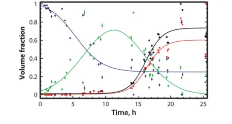
4.12 Time-dependent concentration profiles derived from COSMiCS for each species: monomer, oligomer and fibril. . . 63

4.13 Correlation between ThT signal and concentration of fibril species derived with COSMiCS for insulin. . . 64

4.14 SAXS profiles showing the evolution of fibrillation of αSNE46K . . . 65

4.15 Primary SAXS data analysis for αSNE46K. . . 66

4.16 Principal Component Analysis (PCA) of the complete αSNE46Kdatasets. . . 66

4.17 Optimized results from the decomposition of the αSNE46K data with

MCR-ALS using only the absolute scale data representation.. . . 67

4.18 Optimized results from the decomposition of the αSNE46Kdataset using

MCR-ALS using 4 species. . . 67

4.19 Results of the optimized SAXS curves for αSNE46Kobtained using MCR-ALS

2.0. . . 68

4.20 Representations of the αSNE46KSAXS data measured along the fibrillation.. 70

4.21 Assessment of Outlier Curves in the αSNE46KSAXS Dataset . . . 71

4.22 COSMiCS Analysis of αSNE46KFibrillation with COSMiCS using AHK

com-bination of matrices. . . 72

4.23 A) EOM fitting of the αSNE46K curve isolated with COSMiCS. B)

Distribu-tions of radii of gyraDistribu-tions for the pool of αSNE46K conformations and the

EOM selected ones. . . 72

4.24 Three orientations of the ab initio structure of the fibril repeating unit of αSNE46Kdetermined from the decomposed curve with COSMiCS. . . 73

4.25 Concentration profiles for the monomer, oligomer, and fibril species of αSNE46K

derived from COSMiCS using AHK combination. ThT fluorescence signal superimposed. . . 74

(16)

4.26 Correlation between ThT signal and concentration of fibril species derived

with COSMiCS for αSNE46K. . . 74

4.27 ThT curves of the individual wells from which the samples were withdrawn. 75 4.28 Holtzer and Kratky representations of the decomposed species from COSMiCS for insulin and αSNE46K. . . 77

5.1 COSMiCS flowchart . . . 82

5.2 Example of the order in which COSMiCS loads the files. . . 83

5.3 PCA results for the αSNE46Kdataset. . . 85

5.4 SAXS dataset of αSN plotted in the four representations that will be used by COSMiCS. . . 86

5.5 Selected initial estimations for the MCR-ALS optimization after the sorting. 88 5.6 Graphical output shown and updated during COSMiCS optimization . . . 91

5.7 Example of the final solution corresponding to the AK combination. . . 93

5.8 Example of the resulting optimization after removing an outlier. . . 95

5.9 Screenshot of the output folders and files created by COSMiCS. . . 96

5.10 Screenshot of the report html file (1 of 5) . . . 97

5.15 Crystallographic structures of the monomer (4QHF), dimer (4QHG) and tetramer (4QHH) of the selecase . . . 100

5.16 Complete synthetic dataset of the selecase example in semi-logarithmic scale. 101 5.17 COSMiCS analysis of the selecase dataset. . . 103

5.18 Crystallographic structure of the complex formed by the cytochrome c per-oxidase and the iso-1-cytochrome c used to generate the synthetic titration SAXS dataset. . . 103

5.19 Complete synthetic dataset in semi-logarithmic scale for the transient inter-action between yeast cytochrome c peroxidase and yeast iso-1 cytochrome c.. . . 105

5.20 Results of the COSMiCS analysis of the system A + B ⇀↽ AB for the AK combination, fixing the curves from known species (subunit A and B). . . . 107

5.21 Results of the COSMiCS analysis of the system A + B ⇀↽ AB using just the Absolute values, without fixing curves. . . 108

6.1 Synthetic datasets. A) Synthetic curves computed with CRYSOL for the monomer and dimer. B) Gaussians corresponding to the individual popu-lations of each species simulating a SEC-SAXS experiment. C) Final dataset with noise (σ0.2) in semi-logarithmic scale. D) I(0) of the complete synthetic dataset . . . 111

6.2 Results from PCA for the three synthetic datasets with increasing amount of noise. . . 112

(17)

6.3 COSMiCS analysis for the monomer-dimer synthetic dataset with low signal-to-noise . . . 114

6.4 Results from the COSMiCS analysis of the synthetic SEC-SAXS dataset using the final noise . . . 115

6.5 COSMiCS population profiles for the monomer-dimer synthetic dataset with low signal-to-noise . . . 116

6.6 Results from the COSMiCS analysis of the synthetic SEC-SAXS data using a scale of 0.2 of the final noise . . . 117

6.7 Results from the COSMiCS analysis of the synthetic SEC-SAXS data using a scale of 0.5 of the final noise . . . 117

6.8 Results from the COSMiCS analysis of the synthetic SEC-SAXS dataset using the final noise . . . 118

6.9 Integration of first 50 I(s) points of the SAXS data and original Gaussian populations used to generate the synthetic data. Rg for the three datasets

with different noise levels. . . 119

6.10 EFA of synthetic data (monomer-dimer system) without noise, in the for-ward and backfor-ward directions. . . 121

6.11 EFA from synthetic data (monomer-dimer system). . . 122

6.12 EFA from synthetic data (monomer-dimer system) for the different noise lev-els tested (σ0.2, σ0.5and σ1.0) . . . 123

6.13 Results from the COSMiCS analysis of the synthetic SEC-SAX data using the final noise without scaling, adding an equality constraint obtained using the Rganalysis.. . . 124

6.14 Theoretical and COSMiCS back-calculated Uv-vis absorbance when using the Absorbance data as a closure constraint in the COSMiCS analysis. . . 126

6.15 Results from the COSMiCS analysis of the synthetic low signal-to-noise SEC-SAXS dataset (σ1.0) including an equality constraint that indicates that the

dimer ends at frame 700 and monomer starts at frame 500, and a closure using UV-vis Absorbance information . . . 127

6.16 Results from the COSMiCS analysis of the synthetic low signal-to-noise SEC-SAXS dataset including a closure using the UV-vis Absorbance information 127

6.17 A) Porcine POP in the closed conformation covalently bound to the active-site-directed inhibitor ZPP. B) Aeromonas punctata POP in the open confor-mation. C) Inhibitor ZPP. . . 129

6.18 Size exclusion chromatography coupled to SAXS. Representative SEC chro-matogram of free POP at room temperature . . . 130

6.19 SEC-SAXS integration chromatograms of ZPP-bound POP. . . 130

6.20 SEC-SAXS I(0) chromatogram for the monomer frames of ZPP-bound POP. 131

6.21 Singular Value Decomposition (SVD) of the monomer region of SEC-SAXS I(0) chromatograms at different intervals. . . 133

6.22 A) EOM fitting of the scattering profile of ZPP-bound POP and theoretical curve. B) Guinier plot and Rgvalue. . . 134

(18)

6.23 MD simulations of inhibited POP: MD4 and MD5. POP crystallographic

structure. . . 134

6.24 SEC-SAXS integration chromatogram of free POP . . . 135

6.25 SEC-SAXS I(0) chromatogram displaying peaks I and II of free POP.. . . 135

6.26 Rgand EFA along the SEC-SAXS chromatogram of free POP. . . 137

6.27 Results from the COSMiCS analysis of the SEC-SAXS dataset for free POP. . 138

6.28 Singular Value Decomposition (SVD) of the monomer region of SEC-SAXS I(0) chromatogram of free POP at different intervals . . . 139

6.29 MD simulations of free POP: MD1, MD2 and MD3. X-ray structure of POP in a closed conformation with the inhibitor removed . . . 140

6.30 EOM fitting of peak I.. . . 141

6.31 P(r) function of species corresponding to peaks I and III . . . 146

7.1 Chemical structure and emission spectra of p-FTAA with α-synuclein. . . . 149

7.2 Chemical structure and emission spectra of q-FTAA with α-synuclein. . . . 150

7.3 Chemical structure and emission spectra of h-FTAA with α-synuclein. . . . 151

7.4 Photo of the ProbeDrum set-up. . . 152

7.5 ThT fluorescence spectra of the fibrillation experiment for 8.13 mg/ml αSN and 20 µM ThT . . . 155

7.6 p-FTAA fluorescence spectra of the fibrillation experiment for 8.80 mg/ml αSN and 1.2 µM p-FTAA for the first 4 hours of the fibrillation process. . . . 155

7.7 TEM image from the ProbeDrum fibrillation from a sample of 8.1 mg/ml of αSN and 20 µM of ThT after 24 hours of fibrillation. . . 156

7.8 A) p-FTAA series. SAXS curves of the fibrillation process of αSN at 8.3 mg/ml and 1.2 µM p-FTAA during 10.3 hours. B) SLS intensity at 636 nm. C) Fluorescence spectra from 450 – 720 nm for the first 1.5 hours and from 1.5 to 8.2 hours. . . 157

7.9 TEM image of α-synuclein fibrils in the presence of pFTAA after 10 hours of fibrillation. . . 158

7.10 A) q-FTAA series. SAXS curves of the fibrillation process of αSN at 8.6 mg/ml and 2.4 µM q-FTAA during 8.5 hours. B) SLS intensity at 636 nm. C) Fluorescence spectra from 450 – 720 nm for the 8.5 hours. . . 159

7.11 TEM image that shows the fibrils of α-synuclein in the presence of qFTAA probe after 8.5 hours of fibrillation. . . 159

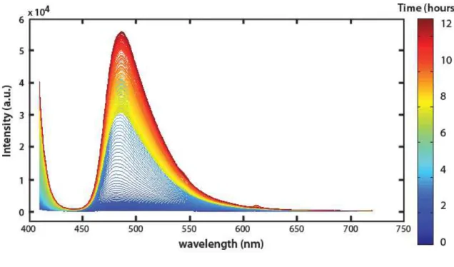
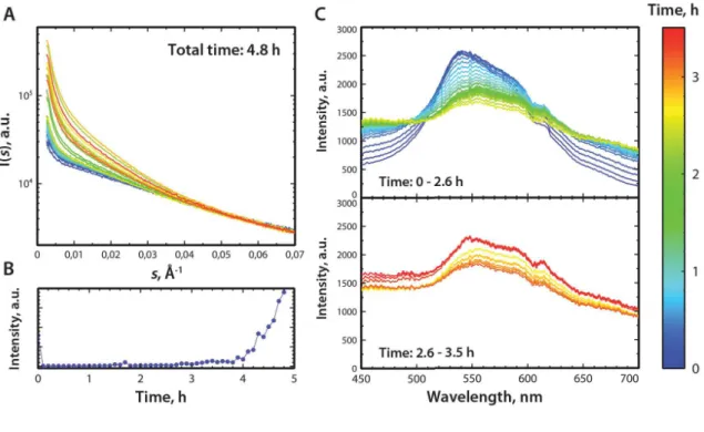
7.12 A) h-FTAA series. SAXS curves of the fibrillation process of alphaSN at 7.3 mg/ml and 1.2 µM h-FTAA during 4.7 hours. B) SLS intensity at 636 nm. C) Fluorescence spectra from 450 – 720 nm for the first 2.6 hours and from 2.6 to 3.5 hours. . . 160

(19)

(20)

List of Tables

4.1 Fitting of the insulin SAXS datasets with COSMiCS using different combi-nations of data matrices. . . 55

4.2 Structural information from the pure species of insulin derived with COSMiCS. 60

4.3 Fitting of the αSNE46KSAXS datasets with COSMiCS using different

combi-nations of data matrices. . . 69

4.4 Structural information from the pure species of α-synuclein E46K derived from COSMiCS. . . 73

5.1 Results of the COSMiCS analysis of the synthetic dataset for the selecase test that has mass conservation . . . 102

5.2 Results of the COSMiCS analysis of the synthetic dataset for titration case representing a transient biomolecular interaction. . . 106

6.1 Analysis of the COSMiCS decomposed scattering curves and concentration profiles from datasets with increasing levels of noise compared with the the-oretical values used to generate the data. . . 113

6.2 Analysis of the COSMiCS decomposed species from datasets with high level of noise using different constraints. . . 125

6.3 Intervals and structures from MD simulations taken for the EOM analysis . 140

7.1 Optimization experiments performed with the ProbeDrum. . . 153

7.2 Optimal selected conditions of the fibrillation experiment for αSN in the ProbeDrum . . . 157

(21)

(22)

List of Abbreviations

αSN α-synuclein

AF Amyloid Fibrils

AFM Atomic Force Microscopy BSA Bovine Serum Albumin CD Circular Dychroism

COSMiCS Complex Objective Structural analysis of Multi-Component Systems Dmax Maximum intra-particle distance

DLB Dementia with Lewy Bodies DTT Dithiothreitol

EFA Evolving Factor Analysis EM Electron Microscopy

EOM Ensemble Optimization Method FSC Fourier Shell Correlation

FTIR Fourier Transform infrared microscopy GA Genetic Algorithm

IDP Intrinsically disordered Protein IDR Intrinsically disordered Region kDa kilo Dalton

LBs Lewy Bodies

MALLS Multi angle laser light scattering

MCR-ALS Multivariate Curve Resolution using Alternating Least Squares MD Molecular Dynamics

MSA Multiple System Atropy MW Molecular Weight

NAC Non-Amyloid-β Component NMR Nuclear Magnetic Resonance PCA Principal Component Analysis PD Parkinson’s disease

POP Prolyl Oligopeptidase p(r) Pair-distance distribution Rg Radius of gyration

SA Simulated annealing

SAXS Small-Angle X-ray Scattering SEC Size-Exclusion Chromatography SLS Static Light Scattering

(23)

SR Synchrotron radiation

SVD Singular Value Decomposition DTT Tris(2-carboxyethyl)phosphine TEM Transmission Electron Microscopy ThT Thioflavin T

WAXS Wide-angle X-ray scattering

(24)

Part I

(25)

(26)

Chapter 1

Small-Angle X-ray Scattering

Small-angle scattering (SAS) of X-rays (SAXS) or neutrons (SANS) is a biophysical method used in many areas of science and technology. In biology, is widely applied for the analysis of macromolecules in solution. SAXS is able to study the overall shape and struc-tural transitions of biological macromolecules in solution. SAXS provides low resolution information on the shape, conformation and assembly state of proteins, nucleic acids and all kinds of macromolecular complexes. In this thesis I will talk about SAXS, which is the method used along this work, but the theory and analysis would be equivalent for SANS.

1.1 Small angle X-ray scattering for proteins

The study of the molecular mechanisms underlying the function of complex biologi-cal systems is often the focus of structural biology [1,2]. The three dimensional structure of a biomolecule determines its functionality in vivo and knowing the 3D structure becomes important when studying the structural bases of biological mechanisms. Small angle X-ray scattering (SAXS) is a powerful method for analyzing the structure and the structural changes of biological macromolecules in solution.

The main advantage of SAXS is that, unlike NMR or X-ray crystallography, does not requires any special sample processing like crystallization, cryo-cooling or isotopic label-ing. The sample is measured in solution, providing structural information in nearly native conditions. This characteristic allows its use not only for static structural modelling but also for the analysis of the response to changes in the experimental conditions (pH, tem-perature, pressure, ionic strength, binding. . . ). It is also possible to follow the time course of processes such as folding/unfolding and assembly/dissociation over several orders of magnitude in time. The capacity of SAXS for studying a protein without need of crystalliza-tion allows characterizacrystalliza-tion of proteins that are impossible to crystallize, like intrinsically disordered proteins (IDPs).

Another important advantage of the technique is that it can be applied to particles in a wide range of molecular sizes, from small proteins or peptides to large macromolecular machines [1,2]. Biophysical parameters such as the radius of gyration (Rg), the maximum intra-particle distance (Dmax) and the molecular weight (MW) can be estimated in an auto-mated way while the data are collected, which makes SAXS also interesting from a practical point of view. The scattering data are also able to provide structural information that can

(27)

FIGURE1.1.Schematic representation of a SAXS experiment

be exploited to derive low-resolution 3D structures. However, SAXS becomes more infor-mative in combination with other structural, hydrodynamic, computational or biochemical methods. In the following sections I will describe the method and its applications.

1.2 General SAXS theory

In a typical SAXS experiment, a monochromatic (with a well-defined wavelength, λ) and collimated (parallel) X-ray beam is directed orthogonally onto a flow cell or static flat sample holder containing the biological sample in solution and a detector is placed on the opposite site of the sample in line with the beam (Figure1.1). The 2D detector is placed at a longer distance between the sample and the detector compared with that used for crystallography in order to detect the scattering from the small angle range.

When the sample is illuminated by the monochromatic plane wave, with a modulus |k| = 2µ/λ, the electrons within the object interact with the incident radiation becoming a source of spherical waves. For elastic scattering, where the energy and wavelength of the incident and scattered radiation are identical, the modulus of the scattered wave is |k’| = |k|. Along this thesis I will consider only the case of elastic scattering, which is the most relevant for structural studies and depends on the momentum transfer, s = k’ – k.

The scattering process involves a transformation from the ‘real’ space coordinates, r, where the structure of the scattering is defined, to the ‘reciprocal’ space of scattering vec-tors, s, in which the scattered radiation is measured. This process is described by a Fourier transformation, which involves a reciprocity between dimensions in real and reciprocal space implying that the smaller the ‘real’ size, the larger the corresponding ‘reciprocal’ size. In solution, the scattering is isotropic and the scattered intensity, Itotal(s), depends only on the momentum transfer |s| = (4µ sinθ)/λ, where 2 is the scattering angle between the incident beam and the direction of observation.

(28)

The scattered waves from each electron have the same frequency and amplitude and can be summed. The intensity measured represents a summation of all the back scattered waves and is proportional to the square of the amplitude A(s), I(s) = |A(s)|2_[₃_{]. To describe}

the scattering of proteins in solution it is convenient to introduce the scattering length density distribution ((r)), that is equal to the total scattering length of the atoms per unit of solution volume [3]. The scattering amplitude is related to ρ(r) by a Fourier transform:

A(s) = !

V

ρ(r)e−isr

dr (Eq. 1.1)

where the integration is performed over the particle volume (V), r is the vector from an arbitrary origin to another point within the sample and s is the scattering length vector. The observed intensity is the product of the amplitude and its complex conjugate:

I(s) = |A(s)|2 = A(s) · A∗ (s) = ! ! V ρ(r)ρ(r∗ )e−is(r−r∗₎ drdr∗ (Eq. 1.2) Proteins in the solution and the bulk solvent have different average electron densi-ties (ρs(r) 0.33 e-1Å-3for water and ρs(r) 0.44 e-1Å-3for proteins). Therefore, the particles are embedded in a homogeneous matrix with a constant scattering density, ρs. As a con-sequence, Eq. 1.1andEq. 1.2should be replaced by the difference between the electron density of the single particle and the solvent, ∆ρ(r) = ρ(r) − ρs(r). The autocorrelation function expresses the correlation between the densities measured at two random points separated by the distance r averaged over the illuminated volume V. The autocorrelation function of the particle γ(r) [4] is defined by:

γ_{(s) ≡ ∆ρ}2(r) = ! V ∆ρ(r′ )∆ρ(r′ − r)dr′ (Eq. 1.3) UsingEq. 1.3,Eq. 1.2can be written as

I(s) = |A(s)|2 = ! V ∆ρ∼₂ (r)e−_isr dr (Eq. 1.4)

We assume here that the solution is dilute enough so that inter-particle interference is negligible, and consequently, a spatial average can be made. This means that the intensity depends only on the magnitude and not on the azimuthal dependence of the s vector, r = |r| and s = |s|. In these conditions,Eq. 1.4can be spatially averaged and results in:

I(s) = #|A(s)|2$ = # ! V ∆ρ ∼₂ (r)e−_isr dr$ (Eq. 1.5)

The scattering intensity recorded in the detector, as an isotropic image, can be ra-dially averaged giving the 1D data by applying the Debye formula [5], #e−_isr

$ = sin(sr)_sr , expressingEq. 1.5as:

I(s) = 4π ! ∞

0

γ(r)r2sin(sr)

(29)

where r is the distance between two scattering elements within the sample.

In practice the generic scheme of a solution SAXS experiment series is starting with the measurement of the empty cell. Subsequently, collecting the scatter of pure water is use-ful for assessing the background level of the camera and for using it for absolute calibration and determination of the molecular weight of the solute. Alternatively, a standard protein can be measure at the beginning of the data collection for the molecular weight (MW); one broadly used standard is bovine serum albumin (BSA) or lysozyme. The use of a standard protein for MW determination will be explained in more detail in section1.2.6. It is very important that the X-ray measurements on solutions of biological macromolecules, both on laboratory instruments and on synchrotron radiation (SR) sources, alternate experiments for the samples and matching solvents, for a correct subtraction of the background. These measurements of the buffer must be done for each sample and in the same cell and close in time to the sample measurements in order to keep identical conditions in both and get a correct background subtraction. The solvent curve is subtracted from the sample data to eliminate the solvent scattering and the instrumental background scattering and obtain the net scattering from the particles (see Figure1.1) [2].

1.2.1 Structure and form factors

The net SAXS intensity after solvent subtraction may be expressed as a product of two terms, Itotal(s) = I(s) · S(s). The form factor, I(s), arises from the scattering from individ-ual particles in solution and contains the information about their structure. The structure factor, S(s), is due to interference of scattered waves emitted by different particles, and con-tains the information about interparticle interactions (about the structure of the solution), which can be either attractive or repulsive. The ideal sample is a monodisperse sample at low concentration to avoid interparticle interference effects and approaches the limit of infinite dilution. This conditions allow analyzing Itotal(s), assuming that S(s) = 1. SAXS is, however, also useful, and actively used, to study interactions between macromolecules in solution based on the analysis of the structure factor S(s) [6].

1.2.2 Goodness-of-fit for SAXS data

The statistical similarity between experimentally obtained intensities, Iexp(s) and those computed from a model Icalc(s) is evaluated using the reduced χ2statistics.

χ2= 1 n − 1 n " i=1 # Iexp(si) − Icalc(si) σ(si) $2 (Eq. 1.7) where n is the number of experimental data points. The resulting χ2 _{for a perfect model} should be in the range 0.9 ≤ χ2 _≥ _{1.1. The experimental error, σ(s}_i_{) must be correctly} estimated in order to have a statistically valid test. This estimation is used in most of the SAXS-based modeling applications and the method chosen along this thesis.

However, a new promising approach for evaluating differences between one-dimensional spectra, has been developed by Svergun and co-workers, called Correlation Map (CorMap)

(30)

FIGURE1.2.Guinier plot for a protein showing good data (left) and aggregation (right)

[7]. This approach, which uses data point correlation, maintains the power of the reduced χ2but has the advantage of being independent of error estimates.

1.2.3 Radius of gyration and forward scattering

The initial slope of the background-corrected scattering curve from a particle can be approximated by a Gaussian function [8] (“Guinier’s law”):

I(s) ≈ I(0)e−s

2 R2_g

3 (Eq. 1.8)

where Rgis the radius of gyration and I(0) is the forward scattering. The Rgcan be derived by plotting the scattering data in a Guinier plot (log(I(s)) against s2_{) (Figure}_1.2_{). The R}

gis then given as the slope of a straight line going through the data points at the low angles. Equation 8 holds in a range of about smax< 1.3, commonly known as the ‘Guinier zone’ or ‘Guinier range’. Depending on the shape of the particles the higher limit can sometimes be larger. Whenever the Guinier plot at low s is not linear, the sample has either aggrega-tion or attractive (upswing) or intermolecular repulsions (downswing), at least in the case of homogeneous particles. Molecules composed of a mixture of different molecules with different scattering length densities also can display an anomalous Guinier behavior.

In the Guinier representation, the intercept of the straight line with the y-axis gives the forward scattering intensity (I(0)). I(0) is proportional to the number N of particles times the square of the product of the particle volume. Since N is inversely proportional to the molecular mass of the particles for a given particle weight concentration, I(0) is propor-tional to the molecular mass, which can be calculated (see more details in section1.2.6).

(31)

1.2.4 Pair-distance distribution

The scattering intensity of non-interacting particles in dilute solution can be de-scribed by an integral that is limited to the maximal dimension (Dmax) in the particles:

I(s)4π

! Dmax

0

p(r)sin(sr)

sr dr (Eq. 1.9)

where r is the distance between two point scatterers within the sample. p(r) is the so-called wise-distance distribution function of the particles. The p(r) can be obtained fromEq. 1.9

via Fourier transform.

p(r) = r 2 2µ2 ! ∞ 0 s2I(s)sin sr sr ds (Eq. 1.10)

Experimental I(s) covers a limited momentum transfer range, and direct Fourier transformation of the scattering curve from this finite number of points is not possible. A solution of this problem is the use of the indirect Fourier transformation [9] that represents p(r)as a linear combination of K orthogonal functions ϕ_kin the range [0, Dmax]:

p(r) = K "

k=1

ckϕk(r) (Eq. 1.11)

The optimal coefficients c_kare calculated through minimization of

Φ = χ2+ αP (p) (Eq. 1.12)

Where χ2_{is the goodness of fit between the experimental data and that calculated by} the direct transform of the p(r) function (Eq. 1.7), and the second term, P(p) ensures the smoothness of the p(r) function (Eq. 1.13)

P (p) =

! Dmax

0

[p′

]2dr (Eq. 1.13)

The regularizing multiplier α balances between the fit to the data and the smoothness of the p(r).

Since the distance distribution is a function in real space, it is often easier to recog-nize features of the particles in the p(r) function than in the scattering curve (Figure1.3). Another important parameter that can be derived from the p(r) is Dmax, the maximum intra-molecular distance, however polydispersity, flexibility and aggregation may influence this parameter. This often results in a Dmaxestimate different than the actual dimension of the scattering particle [10,11].

By definition, p(r) starts with a value of zero at p(0), and it should terminate smoothly at a maximal dimension Dmax. A deviation of p(0) from zero indicates an incorrect back-ground subtraction, which can be used to estimate the backback-ground. A long tail or a shoul-der at the high-r end of the p(r) should induce caution as it may be a sign of aggregation.

(32)

FIGURE1.3.Scattering intensities and pair-wise distance distribution functions, p(r), of geometrical

bodies. Inspired from [12].

Rgcan also be derived from the p(r) through the equation: R2_g = %Dmax 0 r2p(r)dr 2%Dmax 0 p(r)dr (Eq. 1.14) The Rg derived from the p(r) is based on the scattering measured across the entire s range and it is therefore always a good practice to compare Rgderived from a Guinier estimate with the Rgderived from the p(r).

1.2.5 SAXS data representations and their usage

Besides the usual representation of the scattering curve in a semi-logarithmic scale, different representations of the SAXS data have been developed in order to extract addi-tional information. Each representation enhances different features of the particle and it provides useful information1.4.

1.2.5.1 Porod representation

The Porod-Debye law describes a fourth power law approximation to the relation-ship between s and the intensity, I(s) [13,14]. This approximation holds within a limited range of scattering angles and suggests that the scattering of a folded particle decays pro-portionally to s-4_,

I(s) ≈ s−_d_f

(Eq. 1.15) where df describes a fractal degree of freedom, which is shape dependent. For spheres df = 4. The Porod plot I(s)·s4_{plotted against s display a curve asymptotically approaching a} constant value as s approaches infinity. Because Porod’s law assumes uniform density and well-defined borders of contrast for the scattering objects and the solvent, the relationship

(33)

FIGURE1.4.Different representations for a folded protein (BSA), curve blue and from an intrinsically

disorder protein (α-synuclein), red curve. A) Semi-logarithmic scale. B) Holtzer representation. C) Kratky plot. D) Porod plot.

is not fulfilled at high angles where the scattering signal is dominated by higher resolution information.

An estimate of the object volume can also be determined from I(0) and Porod invari-ant Q, irrespective of the nature of the scattering sample:

Q = ! ∞ 0 I(s)s2ds = 2π2 ! V ∆ρ(r)dr (Eq. 1.16)

Q is directly related to the excluded particle volume, and, using that I(0) = (∆ρ)2_V p2,

one obtains

Q = 2π2(∆ρ)2Vp (Eq. 1.17)

The volume of the particle, Porod volume (Vp) [15], is calculated as

Vp= 2π2 I(0)

Q (Eq. 1.18)

(34)

situations, it is often difficult to measure the exact contribution from the solvent. Even a small difference can lead to a different incoherent scattering level. In a plot of I(s)·s4_versus

s4 _{a residual background appears as a slope and 2π(∆ρ)}2_{S/V as the zero intercept. This}

allows estimate a flat background.

Additionally, Porod plot gives also information on the flexibility of the protein [16]. Porod-Debye law predicts a plateau within the low resolution region of the SAXS data when transformed by s4_{. This plateau can be observed in globular proteins but is not} present in unfolded proteins (1.4D).

1.2.5.2 Kratky representation

The Kratky plot [17], where I(s)·s2 _{is plotted against s, is able to qualitatively} dis-tinguish between globular particles and disordered states, and therefore reports on com-pactness. The Kratky plot is routinely used in SAXS data analysis and provides the first estimate of the folded state of the macromolecule. When plotted for globular proteins, where the intensity decays as s-4_{, Kratky plot yields bell-shaped curve with a well-defined} maximum at the smaller angles that fall in the region of higher angles, see Figure1.4. Un-folded proteins show a much slower intensity decay: for example, an ideal random chain decays as s-2_[₁₈_{]. The Kratky plot for unfolded proteins therefore presents a plateau over} a specific range of s, which is followed by a monotonic increase, instead of the peak that presents folded proteins [19]. Partial unfolding or flexibility of the macromolecule lead to an increase of the scattering at higher angles and display an intermediate behavior be-tween that of the folded protein and of the random chain. This graphical representation enhances the relevant features at higher angles and is a very good tool to qualitatively assess compactness, for example, in folding experiments.

1.2.5.3 Holtzer representation

In the Holtzer representation [20] the total scattered intensity is the integrated area of the SAXS data transformed as I(s)·s versus s. This approximation has been recently visited by Rambo and Tainer [21].

SAXS is capable of providing structural information on all particle types, including flexible systems. However, the analysis of the data using the Porod invariant presents lim-itations in the study of these flexible systems. As described above, the Porod invariant is an empirical SAXS value defined for compact folded particles. Q is unique to a scat-tering experiment and requires convergence of the SAS data at high s values in a Kratky plot. Convergence defines an enclosed area where the degree of convergence reflects the compacted (bounded area), flexible or unfolded (unbounded area) solution states. Conse-quently, Q (and therefore, Vp) is undefined for flexible particles. This observation leaves Rgas the only structural parameter that can be reliably derived from SAS data on flexible systems. Unlike the Kratky plot, the integral of I(s)·s versus s converges for both folded-compact and unfolded-flexible particles. Holtzer plot allows deriving a SAXS invariant,

(35)

the Vc. Vcis defined as the ratio of the particle’s zero angle scattering intensity, I(0), to its

total scattered intensity:

Vc = I(0)

% sI(s)ds (Eq. 1.19)

Vc, like Rg, can be calculated from a single scattering curve and is concentration

independent. This value can be used to derive the molecular weight of the particle (see next section).

1.2.6 Calibration to absolute scale and molecular weight

The aim of a scattering experiment is to obtain structural information about the sam-ple. In the case of biological macromolecules this includes the knowledge of the molecular weight (MW) and, therefore, the determination of the oligomeric state. This can be per-formed in several ways.

1.2.6.1 Forward scattering of standard proteins

Standard proteins of known MWs (such as cytochrome C, lysozyme or bovine serum albumin) are often employed to determine the experimental MW of the given protein from the forward scattering, I(0). The standard protein is measured in similar conditions to the protein and the MW can be calculated using the ratio:

M Wp = M Wst·

I(0)p/cp

I(0)st/cst (Eq. 1.20)

where I(0)p, I(0)st are the scattering intensities at zero angle of the studied and the

standard protein, respectively, MWp, MWst are the corresponding molecular weight and

cp, cstare the concentrations.

1.2.6.2 Forward scattering of water

Alternatively, scattering from water can be used to obtain the scattering from the solute in the absolute scale [22, 23] and then to calculate the MW. The water sample is measured in the same cell as the protein samples, and the scattering from the empty holder is subtracted.

1.2.6.3 Porod volume

It is possible to derive the MW from the Porod volume described above. The exact re-lationship between MW and Vpvaries for different proteins depending on a combination of several factors, e.g. particle anisometry, flexibility etc. Using an empirical approach, Sver-gun’s group [15] found that the scattering data range up to about smax= 8/Rgis optimal for a reliable computation of Vp. This upper limit in most cases approximately corresponds to the second minimum in the Porod plot. Using this interval, the average ratio between MW and Vpis 0.625, therefore, the volume in nm3is typically 1.6-2.0 times the MW in kDa.

(36)

1.2.6.4 Ab initio modeling

A similar approach to the Porod volume method is using the particle volume ob-tained from the volume of the low resolution structure of the molecule, which is 2 times the MW in kDa. The low resolution structure can be derived from several programs and it will be explained in more detail in next section.

1.2.6.5 Apparent volume

Fischer described a method to determine the molecular weight of proteins in dilute solution by using the experimental data of a single small-angle X-ray scattering (SAXS) curve measured on a relative scale [24]. This procedure does not require the measurement of SAXS intensity on an absolute scale and does not involve a comparison with another SAXS curve determined from a known standard protein. However, it is necessary an ac-curate determination of the protein concentration. The method is able to derive the MW from the value of the apparent volume V’ derived from truncated experimental SAXS data, using an empirical ratio. A program was developed to implement this technique, making it easily available to the scientific community. The web tool ‘SAXS MoW’ is available at

http://www.if.sc.usp.br/ saxs/. 1.2.6.6 Volume of correlation

The above described methods to determine MWs require the knowledge of the pro-tein concentration, the assumption of a compact near-spherical shape, or SAXS measure-ments on an absolute scale. Recently a new approach was developed to estimate MW of biomolecules without these restrictions. The new method was developed by Rambo & Tainer [21] and is based in the Holtzer representation. The approach determines that a pa-rameter, QR, defined as the ratio of the square of Vc to Rgwith units of Å-3is linear versus molecular mass in a log–log. The linear relationship is a power-law relationship given by

mass = (QR ec )

1/k _{(Eq. 1.21)}

that yields the empirical mass of the scattering biological particle allowing for the direct assessment of oligomeric state and sample quality. Parameters k and c were empirically de-termined and are specific for different classes of macromolecular particles. Vc and Rgare both contrast and concentration independent, thus the determination of molecular mass using QRcan be made from SAXS data collected under diverse buffer conditions and con-centrations. Vc can be calculated with the software ScÅtter, developed by Robert Rambo [21].

1.2.7 Radiation damage

One fraction of the X-rays that interact with the sample is absorbed by the particles damaging their structure. This radiation damage can be neglected in laboratory sources but has become a real program in SR sources due to their high brilliance [25]. The major

(37)

effect of radiation damage in SAXS is radiation-induced aggregation. The aggregates are readily seen in the low-s region of the scattering patterns and can produce erroneous data that are impossible to analyze. Therefore, it is important reduce the radiation damage.

One way to reduce radiation damage is to use a flow cell where the solute is con-stantly flowing through the irradiated volume. A disadvantage of this approach is the need for larger amounts of material.

Another option is the use of additives, such as DTT or TCEP, but is not always pos-sible, as they can reduce disulfide bonds in proteins. A universal approach, employed at nearly all modern SR stations, is to slice the data collection into individual successive time frames (for example, ten or twenty). The recorded patterns are then processed separately and compared to each other (essentially to the first frame), and these frames showing sys-tematic changes are not included in the subsequent averaging and further data processing. This analysis is normally done automatically using standard statistical criteria.

1.2.8 Resolution of SAXS data

Most of the intensity scattered by an object of linear size d is concentrated in the range of momentum transfer up to s = 2µ/d. It is therefore assumed that if the scatter-ing pattern is measured in reciprocal space up to smax it provides information about the

real space object with a resolution ∆ = 2π/s. For spherically averaged scattering patterns from solutions, I(s) usually decays rapidly as a function of momentum transfer, and only low-resolution patterns (d » λ) can be obtained. It is thus clear that solution scattering can-not provide information about the atomic position but only about the overall structure of macromolecules in solution.

The s range used for a SAXS experiment determines the molecular dimensions that can be observed. At a typical beamline the s range is 0.006 Å-1 _{– 0.5 Å}-1 _{and the real}

di-mensions accessible are then 160 Å – 13 Å. Although in theory would be possible to record scattering from macromolecular solutions up to 0.2 nm, the weak SAXS signal that results from scattering events at the high-s range is not much higher than the level of the noise associated with the technique.

The maximum observable dimension is set by the incoming beam, the beam stop size and the collimation of the beam to avoid divergence of the beam around the beamstop area and the area for small angle detection. When the data are recorded, the Rgestimate dictates

the upper limit of the small angle resolution point.

A method very similar to SAXS, Wide-angle X-ray scattering (WAXS), allows access to higher resolution structural information [1,26]. In this technique, the detector is moved closer to the sample to capture X-rays scattered to higher angles. It is even possible to si-multaneously acquire SAXS and WAXS data by placing a detection window near the sam-ple [27]. Although WAXS is easy to implement experimentally, the computational tools required to extract all the information are still under development, and usually it is nec-essary high resolution models are necnec-essary for interpretation of the data. The strength of WAXS lies in its high sensitivity to small changes, and this can, therefore, be applied to identify structural similarities and characterize structural fluctuations. Currently, WAXS is

(38)

employed to study structural fluctuations and ligand binding in proteins [28]. WAXS has been also used to study nucleic acids using molecular dynamics (MD) simulations [29].

1.3 Structural interpretation of SAXS data

Besides providing information on the biophysical parameters such as Rg, Dmax and MW, SAXS analysis of a protein system can provide information about 3D structure, the oligomeric distribution and the flexibility. SAXS data can also be combined with high-resolution structural information, to obtain structures of multi-subunit systems and is rou-tinely used for the validation of structural models obtained by others methods, such as X-ray crystallography, Nuclear Magnetic Resonance (NMR) or Electronic Microscopy (EM). The measured intensity from an ideal monodisperse system is directly related to the single-particle scattering and provides low-resolution structural information of the molecule. However, some of the biological systems present polydispersity, where particles of differ-ent size, shape and/or conformation coexist. To characterize such systems, differdiffer-ent data analysis methods are required. These methods will be described in the following sections.

1.3.1 Structural analysis of monodisperse biological systems

In monodisperse systems one considers that an individual species in a single con-formation is present in solution. Although biomolecules experience dynamic phenomena at multiple levels, when these motions do not perturb the overall size and shape of the particle, they are not probed by SAXS and the system can be considered as monodisperse. Several approaches to structurally characterize monodisperse systems have been reported depending on the additional information integrated in the analysis.

1.3.1.1 Ab initio modeling

The aim of ab initio analysis of SAXS data is to recover the three-dimensional structure of the molecules in solution from the one-dimensional scattering pattern. The reconstruc-tion of a 3D model of a molecule from its one-dimensional scattering pattern is a challeng-ing task and different approaches have been developed.

The first ab initio shape determination method was proposed in 1970 by Stuhrmann [30]. The particle shape was represented by an angular envelope function describing the particle boundary in spherical coordinates. The method was implemented much later in the program SASHA [31], which was the first available shape determination program for SAXS. The spherical harmonics formalism proved to be very useful for analysis of SAXS data and it has been employed in many other approaches. The use of the angular envelope function is limited to relatively simple shapes without internal cavities. More detailed ab initioreconstructions became possible with the development of bead-modeling approaches [32]. A spherical volume with diameter Dmax, which is obtained from the scattering pat-tern through p(r), is filled with M densely packed beads (spheres of much smaller radius r0). Each of the beads may belong either to the particle (index = 1) or to the solvent (index

(39)

= 0), and the shape is thus described by a binary string X of length M. Starting from a ran-dom distribution of 1s and 0s, the model is ranran-domly modified using a Monte Carlo-like search to find a string X fitting the experimental data. The original bead method, program DALAI_GA ([32], uses a genetic algorithm and does not impose explicit constrains. The program DAMMIN (Dummy Atom Model Minimisation) [33] is the most popular ab initio bead-modeling program. The program uses a random initial approximation by simulated annealing (SA) procedure [34]. The discrepancy (χ2_{) is evaluated between the} experimen-tal and calculated scattering intensities. At each step in the SA procedure the assignment of a single bead is randomly changed leading to a new model X’. The solution is constrained to ensure compactness and connectivity of the resulting shape. A new optimized version of the program was implemented in the software DAMMIF [35], which perform this opti-mization in a faster manner.

One inherent problem of the shape determination methods is the uncertainty. In other words, different starting points yield different structural models with essentially the same fit to the data. To achieve a good solution is a recommendable approach to run shape determination programs several times to produce a diverse set of models corresponding to nearly identical scattering curves and inspect how different these models are as an in-dicator of the stability of the reconstruction. The uniqueness of the reconstruction is then assessed by a posteriori comparison and averaging of the different models. A new a priori ambiguity measure has been recently developed, based on the number of distinct shape categories compatible with a given dataset [36]. The models obtained in independent runs can be superimposed and averaged to obtain a most probable model, which is automated in the program package DAMAVER [37]. The ATSAS package employs the program SUP-COMP [38], which aligns two (low or high resolution), structural models represented by ensembles of points and yields a measure of their similarity. All pairs of independent models are aligned with SUPCOMP, and the model giving the smallest average discrep-ancy with the rest is taken as a reference model. Then, a density map of beads is computed and cut at a threshold corresponding to the excluded particle volume.

The reliability of ab initio models can be further improved if additional information about the particle is available. In particular, symmetry restrictions permit to significantly speed up the computations and reduce the discrepancy among models.

It is also important establish the resolution of ab initio shape modelling. A resolution based on analysis of the average Fourier shell correlation (FSC) functions within an ensem-ble of constructions has been developed recently by Svergun and co-workers [39]. This method has been implemented in the ATSAS suite in a program called SASRES [40] and it is able to determine resolution of ab initio models obtained using alternative procedures. 1.3.1.2 Computation of scattering patterns from atomic models

SAXS is often used for validation of 3D models obtained by high resolution methods, such as X-ray crystallography, NMR or homology models. Different methods have been developed to compute intensity profiles from a particular macromolecular structure. These methods are based on the Debye equation described above or on spherical harmonics.

(40)

Probably the most popular approach to compute SAXS intensity profiles from atomic coordinates is CRYSOL [41], and is the method used in this thesis. In CRYSOL, the scat-tering body is expanded in terms of an infinite series of spherical harmonics. One of the features of this method is the consideration of a homogeneous hydration shell surrounding the target.

Water modeling is critical to the correct interpretation of SAXS profiles and the more advanced approaches include the explicit modeling of the solvation shell. Programs such as the package PHAISTOS [42], AXES [43], SAXSTER [44], SASTBX [45] or AquaSAXS [46] implement different methods to compute the scatter profile and the solvent shell. The web server FoXs [47] is a tool for several SAXS-based modeling applications, including the com-putation of a SAXS profile of a given structure. The software also models the first solvation layer based on the atomic solvent accessible areas and provides an optimization of the hy-dration layer density as well as the excluded volume of the protein, to maximize the fit of the computed profile to the experimental profile. A new web server, called WAXSIS [48], was released recently. This approach computes SAXS (and WAXS) curves based on explicit-solvent all-atom molecular dynamics (MD) simulations. The MD simulations pro-vide a realistic model for both the hydration layer and the excluded solvent. More detailed information about the different methods can be found in [49].

1.3.1.3 Rigid-body modeling

The strength of SAXS is further revealed in hybrid approaches in which this tech-nique is used in combination with other structural information. Rigid body modeling ap-proaches utilize atomic models of individual subunits or domains obtained by high reso-lution methods to analyze the structure of a complex or multidomain protein in soreso-lution. The scattering amplitude of the subunits can be precomputed with the methods described in the previous section and they are moved and rotated with respect to each other to find the configuration that fits better with SAXS data. A number of automated approaches have been developed using SAXS to determine the positions and orientations of subunits within macromolecular complexes.

One of the most used programs is SASREF [40,50], which, starting from an arbitrary positioning of subunits, conducts random rigid-body movements and rotations, using SA to search for the best fit of the computed complex scattering to the experimental data. SAS-REF add penalties to avoid solutions without physical sense and allows the simultaneous fitting of multiple scattering curves. Moreover, it is possible improve its results by using in-formation from other techniques, such as symmetry, orientational constrains, inter-residue contacts and inter-subunit distances. SASREF performs an automated global optimization of multi-subunit complexes, but the ATSAS suite includes other programs that comple-ments SASREF, like BUNCH [40], used for multi-domain assembly; and the combination of both, CORAL [50].