Publisher’s version / Version de l'éditeur:
Vous avez des questions? Nous pouvons vous aider. Pour communiquer directement avec un auteur, consultez la première page de la revue dans laquelle son article a été publié afin de trouver ses coordonnées. Si vous n’arrivez pas à les repérer, communiquez avec nous à PublicationsArchive-ArchivesPublications@nrc-cnrc.gc.ca.
Questions? Contact the NRC Publications Archive team at
PublicationsArchive-ArchivesPublications@nrc-cnrc.gc.ca. If you wish to email the authors directly, please see the first page of the publication for their contact information.
https://publications-cnrc.canada.ca/fra/droits
L’accès à ce site Web et l’utilisation de son contenu sont assujettis aux conditions présentées dans le site LISEZ CES CONDITIONS ATTENTIVEMENT AVANT D’UTILISER CE SITE WEB.
Internal Report (National Research Council of Canada. Institute for Research in Construction), 1998-05-01
READ THESE TERMS AND CONDITIONS CAREFULLY BEFORE USING THIS WEBSITE.
https://nrc-publications.canada.ca/eng/copyright
NRC Publications Archive Record / Notice des Archives des publications du CNRC :
https://nrc-publications.canada.ca/eng/view/object/?id=2154cda5-5899-4dc7-a142-d89db79b107b https://publications-cnrc.canada.ca/fra/voir/objet/?id=2154cda5-5899-4dc7-a142-d89db79b107b
NRC Publications Archive
Archives des publications du CNRC
For the publisher’s version, please access the DOI link below./ Pour consulter la version de l’éditeur, utilisez le lien DOI ci-dessous.
https://doi.org/10.4224/20375571
Access and use of this website and the material on it are subject to the Terms and Conditions set forth at Comparisons of Multizone Airflow/Contaminant Dispersal Models
http://irc.nrc-cnrc.gc.ca
Com pa risons of M ult izone
Airflow /Cont a m ina nt Dispe rsa l M ode ls
I R C - I R - 6 9 8
W a n g , J . ; Z h a n g , J . S . ; S h a w , C . Y . ; R e a r d o n ,
J . T . ; S u , J . Z .
COMPARISONS OF MUL'XTZONE AERFLOW/CONTAMLNANT DISPERSAL MODELS
ABSTRACT
This paper compares the inputloutput routines, algorithms and applications of three well- known multizone airflow models, BREEZE, COMIS and CONTAM. It was found that all three
models used similar atgorithrns to solve a set of non-linear flow equations, and are capable of
simulating air and contaminant transport in Iarge buildings. The three models differed considerably i n interface provided for the inputloutput routines. As a test case, the three models
were used to predict the air and contaminant distributions i n a five-storey apartment building. The model predictions agreed well with each other. They also agreed with the field measurements in general.
INTRODUCTION
Multizone models are widely used to study air and contaminant movement in buildings. There have been two comprehensive reviews of rnuItizone models (Feustel and Kendon 1985,
Feustel and Dieris 1992), which covered fifty models, Based on these reviews, three were
selected for further comparison: BREEZE (version 6.0c, BRE, 1993), COMIS (version 1.3,
+. Feustel and Smith, 1994) and CONTAM (version 94, Walton, 1994). All three models are able to handle a Iarge number of zones which is essential for large building applications.
In this paper, we first provide a comprehensive comparison of the main features such as
the representations of zones, flow paths, driving forces, algorithms and inputloutput routines. We
then compare the results of the airflow and contaminant flow patterns predicted by the models
in a five-storey apartment building. Predictions are also compared with measured data. More
details of the model features and predictions can be found in an IRC report (Wang, et aP., 1995).
GENERAL COMPARISONS OF MODELS
The main features of the three models are summarized in Table 1. In general, all three
multizone airflow models use a network approach which includes two basic elements: a zone
(node) and a flow path. Spaces and shafts of a building are represented by zone which are linked together by flow paths. By conducting a mass balance at each zone (i) and applying a flow path
The pressure in each zone (P) and the resultant airflow rate through each flow path (qj)
can be calculated by using an iteration technique (see algorithm section later). Based on the
airflow rates, the contaminant concentrations in each zone can then be calculated.
Zones
In all three models, a zone can represent a single cell (space), a shaft (multi-layer zone)
or an HVAC system.
The basic input data for each zone required by the three models include: zone name,
volume, temperature, and initial contaminant concentration. In addition to zone names, COME
also requires the user to input a zone ID and a reference height for each zone. A set of default
values are also provided by the three models (e.g., initial concentration in each zone is assumed to be zero in
COMTS
and CONTAM). BREEZE calculates each zone volume from the scaleddrawing of the floor plan while COMIS and CONTAM require the user to input the value directly.
Flow Paths
Flow paths are used to link two adjacent or non-ad+jacent zones. Flow paths can be
classified into two types: fan flow paths and basic flow paths.
Fan Flow Paths. A fan flow path is used to describe an airhandling system or an airflow
system with a known airflow rate. For an airhandling system, a cubic polynomial curve is used in the three rnodeIs to describe the q-AP relationship, as:
BREEZE requires the user to input the four coefficients {A, B, C, and D) manually. Yn
COMIS, the user can either input the four coefficients directly or input a maximum of 8 pairs of measured airflow-pressure data which will be used by the program to calculate the four
coefficients. CONTAM allows a minimum of 4 pairs to a maximum of I0 pairs of measured
airflow-pressure data to be input to determine the four coefficients. For an airflow system with
a know airflow rate (e.g., a fan with a constant airflow rate), BREEZE and COMIS require the user to specify the flow coefficients. CONTAM uses a "constant flow path" to accommodate
such an input.
To reduce input efforts, COMIS and CONTAM allow the use of a pre-defined common
fan flow path to define the fan flow paths which have the same performance curve. Furthermore,
COMIS and CONTAM estimate the air leakage through the gaps of closed dampers in an
airhandling system in the same way as that through a crack (i.e, a basic flow path) when the fan is off.
Basic Flow Paths. A basic flow path is used to describe openings and cracks existed in
walls and around windows/doors. The flow rate through the basic flow paths is described by the
power law equation (Eq.(3)),
The input parameters for each flow path are the flow coefficient (C,) and exponent (n).
The sign which determines the direction of the airflow through the flow path is chosen according
to the pressure difference across the path. Tn addition, BREEZE and CONTAM have the options of using the following equations (Eq.(4) and (5)) for calculating such flow rates:
for BREEZE and
for CONTAM, respectively.
Similar to the fan flow path input, both COMTS and CONTAM allow the use of a pre-
defined common flow path to define the basic Row paths which have the same flow coefficient
(C,) and the same exponent In). To further reduce input efforts, CONTAM also provides a
modifier to calculate the flow coefficient (C,) for the flow path whose exponent is identical to that of the common flow path.
Presentation of Wind Pressures and Thermal Buoyancy
There are three driving forces which determine the air and pollutant movements in a building: the operation of airhandling systems (i.e., the fans), wind pressure and stack effect. As
discussed above, in all three models the operation of the fans are modelled simply by applying
a cubic polynomial curve (Eq.(2)). However, the presentations of the wind pressures and stack effect are different from model to model.
Wind Pressure. In general, the wind-induced pressure difference across a flow path
connected to the building envelope i s simply described by the following equation (Eq.(6)),
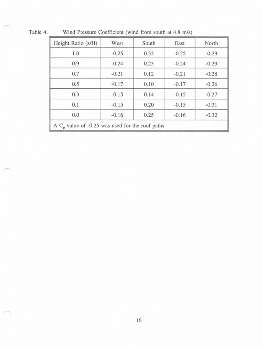
Tn BREEZE, for simulation involving a single wind direction only, the C, value of each
involving multiple wind directions, the C, value of each of such flow paths for different wind directions are input using a table form and saved as an independent file. The input file includes
both the horizontal and the vertical profiles of wind pressures exerted on the building envelope. In CONTAN, the wind pressure acting on each flow path for each wind direction can be
input directly (manual pre-calculation of the wind pressure is needed). Alternatively, the user can input a set of C , values from up to 16 wind directions to calculate the wind pressures for
paths at the same building height.
Tn addition to manual input for C,, as one of the major contributions to the multizone airflow modelling, COMIS includes a sub-routine to automatically calculate. the C , values at any
location of the building envelope for any wind angle. The calculation of C, requires a description of urban environments, surrounding Iayout, building dimensions, building shapes, and the Iocations of leakage openings in the building envelope. At present, the application of the
sub-routine is restricted to few specific cases (e.g., regular building shape and low terrain
roughness). Furthermore, in COMIS the reference wind speed (U) is calculated by a sub-routine that converts the wind profile (which are input explicitly) measured at a weather station to a specific wind profile on site. The calculation needs two sets of data: (1) at weather station:
Reference height for the wind speed, Altitude of the station and Wind speed profile exponent; (2)
on-site: Plan area densiry, Surrounding building height and Wind speed prqfife exponent (an
exponent in the power law function of the wind veIocity profile).
In BREEZE and CONTAM, the reference wind speed (U) must be input directly.
Stack Effect/Temperature Gradient. All three models use the following equation to calculate the stack effect pressure at a height (h) relative to a reference point of a building (i.e., floor level):
The air density is calculated from the temperature and ambient pressure. The temperature in a single storey zone is generally considered to be uniform. However, BREEZE allows the
temperature to vary vertically in a shaft (zones with a height greater than one storey) while
CUMTS uses a constant temperature gradient in each zone. Similar to BREEZE, CONTAM also
allows the temperature to vary in a shaft when the shaft is modeHed as a number of zones stacked one above the other.
Additionally, heat sources (e.g., a heater) and sinks (e.g., a cooling coil) are considered
in
BREEZE
and, therefore, the temperature in each zone is determined by conducting an energybalance. In COMIS, the temperature in each zone can be controlled using a specified
temperature profile (temperature schedule). In CONTAM, neither heat source nor heat sink in
each zone is included.
The temperature difference can also cause two-way airflows across a large opening such
as a doorway. All three models are able to calculate such two-way airflows. The flow rates through a two-way path are calculated by integrating the flows calculated from the power law
equation (Eq.(3)) over the height of the opening.
Contaminant Transport Models
In paraIIel with the multizone airflow models, all three models have included a multizone pollutant transport model to predict the contaminant concentration in each zone. All three models assume that the contaminants in each zone are well mixed with the indoor air, except that BREEZE allows the contaminant concentrations in a shaft to vary with the floor level.
CONTAM has the same flexibility if a shaft is modelled as several zones stacked one on top
another. The contaminant concentration in each zone is calculated by solving the mass balance equations.
In addition, BREEZE can model the contaminant generation and decay rates that vary exponentially with time in each zone. COMIS uses a constant coefficient model (i.e., constant
generation or sink rate). CONTAM provides the user with 5 SourcelSink models to simulate different contaminant activities, namely, Constant Coefficient model (constant rate), Pressure
Driven model (for contaminant sources which are governed by the inside-outside pressure
difference, such as radon or soil gas entry into basement), Cutoff Concentration model (for same
volatile organic compounds their emission would stop after a period of time), Exponential Decay Source model and Boundary Layer SourceISink model (Axley, 1990, 1 99 1). Additionally, a
kinetic reaction effect (with constant rate) is also included for each zone in CONTAM to account for some chemical reactions. The maximum number of contaminants which can be defined are 1, 5, and 10 for BREEZE, COMIS and CONTAM, respectively. Furthermore, a pollutant filter is also provided for each path in COMIS and CONTAM so only a fraction of contaminants (from 0 to 100%) can be passed from one zone to another, to simulate the effect of air cleaning device.
Dynamic Simulation
All three models allow predictions of the airflow rates and contaminant concentrations
over a period when temperatures, wind directions and other parameters vary with time. BREEZE uses a control database file for such purpose, while C O M E provides users with a set of path and zone schedules to describe the operation of the equipments (windows, fan, heating, humidifierlde- humidifier), scheduled activity (sourcelsink effect, occupant.), and weather profiles. Similarly,
in CONTAM the conditions of all the paths and zones including the airhandling systems and openings can be changed with time by using a time-control profile. However, CONTAM restricts
the transient simulation to a period of 24 hours only. It is expected that the newer version will allow simulating a longer period of time.
Algorithm (Equation Solves)
The algorithms used in dl three models for solving the system equations (Eq.(l]) are based on the Newton-Raphson method, which uses an iteration technique to calculate
the pressure at each zone and flow rate through each flow path. In general, the pressure (P,) at each zone is calculated by the following equation:
where
J(P,-,
S
- - the system Jacobian matrix, i.e., the derivatives of f(P,.,).The iteration is started by assuming an initial pressure (P,-,) at each zone. The pressure (P,) is then used to calculate the flow rate through each flow path. A mass balance in each zone is checked after each iteration. The iteration continues until the mass balance in each zone satisfies the convergence criterion.
The o in Eq.(8) is called the relaxation coefficient which is introduced to improve the rate of convergence. The selection of w depends on the building characteristics and environmental conditions. As shown in Table 1, BREEZE uses the N-R method (w=O) while COMIS and CONTAM use the modified N-R method ( O < w 1 ) . The Steffesen method which was developed by Walton (1993) was also used in COMIS. It is similar to the N-R method except that the
Steffesen method utilizes two or three steps of previous iterates (P,,., and P,,, or P,-,, P,_, and P,.
,) to obtain the next value (P,,).
Input and Output
Both BREEZE and CONTAM provide the user with a graphical interface for input. Using
a Sketchpad, the data of each level can be copied into a new level. This feature is particularIy useful for tall buildings where the inputs for each floor Ievel are often similar. A major difference between the two programmes is that BREEZE calculates the zone volume based on the scaled floor plan, while CONTAM uses an unscaled drawing and requires the user to input the zone volume explicitly. Additionally, both BREEZE and CONTAM display the input data
on the floor plan and, therefore, are more convenient for user to check the input data. The
graphical interface, while not available for the COMIS program used in this study (version 1.3), - IT
has been included in the later version (version 2.13.
CONTAM. The pressure and flow rates can be displayed on the floor plan. Furthermore, in
CONTAM the concentrations, normalized by the peak value, can be graphically viewed over the simulated period. In BREEZE both the text and graphic image on the screen can be saved to a
graphic (TIFF) file, while in CONTAM the drawing of each floor (rather than whole screen) is output into a graphic (PCX) file.
A CASE STUDY
Simulation Conditions and Experimental Data
Figure 1 shows the layout of a building (Shaw et al. 1991) selected for the simulation.
The building was selected because it represents a typical high rise apartment building and, some test data are available for a preliminary comparison with model results.
As shown in Figure 2, the building consists of 6 floors including a basement and is 12.5 m high (2.5 m for each floor). The north facade of the building is fully exposed and other three
facades are surrounded by buildings of similar height (H=12.5 m). The ground floor garbage room (GBRM) is connected directly to the garbage chute which opens to the corridor of each floor. The garbage chute is opened to the outside through a hatchway in the roof. The garbage
room also has an exhaust fan to exhaust the air directly to the outside. The ventilation shaft is
located at the centre of the building which supplies the outdoor air to the corridor of each floor. There are no return air ducts in this building. A dampered opening, however, exists in the bottom of the building's air handling unit through which some of the interior air can enter the HVAC system. Also, the outdoor air is ducted to the air handling unit.
In this study, two sets of test data were used: airtightness values and contaminant flow
patterns (Shaw at el., 199 1). The measured overall and component airtightness values were used to determine the leakage areas in the building envelope and internal partjtions (in addition, the
total HVAC fresh supply flow rate was also measured and was used to determine the HVAC supply flow rate to each corridor). The tracer gas test results were used to compare with the model predictions.
The contaminant-flow patterns in this building were measured under winter conditions (with an ambient outdoor air temperature condition of 1 I "C and 4.8 m/s wind speed from the
southeast first and then changed to the south shortly after the tracer gas injection). During the
test period, a small amount of tracer gas (SF,) was injected into the ground floor garbage room
(GBRM) to simulate the contaminant and samples were taken at selected locations (the corridors
and the individual apartments) in every floor. The tracer gas experiment has been fully described
earlier (Shaw, Reasdon, Said and Magee 1991 ; Shaw, Magee, and Rousseau 1991).
It shoutd be noted that because the experiments were not designed to obtain data for
model d i d a t i o n , some assumptions still need to be made for the simulation. Therefore, the focus here was to compare the predictions of the three models, while the comparison between the predicted and the measured resuIts can only be seen as preliminary and quaIitative validation
of the models,
Representation of the Building
The following assumptions were made to simplify the building configuration in this study:
1. no air leakage through floorkeiling (concrete assembly floor slabs);
2. no leakage through the HVAC ducts;
3. no air leakage through the elevator shafts;
4. exhaust fans in kitchens and bathrooms were off;
5. the air temperature inside the building was assumed to be uniform at 20 "C.
For the basement and the ground floor, only half (west side) of the floor was included
(Figures 3 and 4) in this simulation because the front (east) side was completely isolated from
the rest of the building (Shaw et al., 1991). For simplicity, the reminder of the basement was treated as one open space. At the ground floor, the 6 apartment units were treated as 6 individual zones. Similarly, for the upper (2-5) floors, the 12 apartment units at each floor were represented by 12 individual zones. In total, there were 65 zones, including 54 apartment units, 6 corridors,
1 open space and 4 vertical shafts (2 stairwelFs, 1 garbage chute, and I ventilation shaft). Figures 3-6 show the basic configurations for the building, and the leakage opening areas
(m2), measured flow rates (k@) and the zonal volumes (m'). The temperature in each zone was assumed to be 20 "C. The initial contaminant concentration was zero, except in the garbage room where a measured initiaI concentration of 5500 ppb was used. It should be pointed out that
since BREEZE depends on the user-specified scaled drawing to calculate the zonal volume, the values calculated by BREEZE were input into the other two programs so that all three models used the same zonal volumes. These zonal volumes may be slightly different from the real zonal volumes, but the differences were estimated to be within 5 % of each other.
As shown in Table 2, a total of 21 1 paths were used, including 9 fan flow paths defined
by the fan flow model (Eq.(2)$, and 202 general openings (77 exterior and 1 25 interior openings)
defined by the power law equation (Eq.(3)), respectively.
Table 3 shows the equivalent orifice areas A, for the total exterior walls of each floor. The A, values for the exterior walIs were calculated from the measured airtightness data of the
building by assuming n=0.5, Cd=0.6 and p=1.205 kglm! The individual A, values of each flow
path on the exterior walls shown in Figures 4-6 were then calculated based on the floor plan by
assuming uniform leakage per unit surface area of the building envelope. Table 3 also shows the measured orifice areas A, for the stairwells and some interior partitions (RM304-RM305 and
RM3 10-RM31 I ) at the third floor. The stair-shaft leakage area and the stair door leakage area were combined for each stair-shaft: the north and south stairwells had a leakage area equivalent to 6 and 7 apartment doors, respectively. The orifice areas for the other internal partition openings shown i n Figures 4-6 were all estimated based on the measurements. These include areas of openings through the garbage chute to the corridors, areas of cracks through the
apartment doors and areas of leakages through the interior partitions.
It should be noted that for n=0.5, the A, values (in Eq.(4j and ( 5 ) ) used by BREEZE and
CONTAM are the same. The C, values used by COMIS were calculated by equating Eq.(3) to
Eq.(4) or (5). This ensured that the actual flow path equations were the same for the three modeIs despite the differences in the input format.
The building's ventilation system supplied the outdoor air to the corridor of each floor. Since only the total outdoor air supply rate was measured, it was assumed the total ventilation rate was uniformly distributed to (through 'Tan flow paths") the corridor of each floor (Figures
3-6). The return flow rate to the air handling system was not measured but was resumed to be 8% of the total ventilation flow rate based on the design plan (Figure 3).
Figure 2 shows that the intake of the ventilation system and the outlet of the exhaust fan
of the garbage room are located on the same side of the building and, with a distance of about
3 rn apart from each other (horizontally the HVAC intake is Iocated at the north side of the
exhaust fan). Therefore, it was very likely that the contaminated air exhausted from the garbage
room would re-enter into building through the ventilation system during the tracer gas test when
the wind came from the South. Because no measurements were made to determine the re-
entering airflow rate, a moderate 10% of the total contaminated airflow exhausted from the
garbage room was assumed to re-enter the building through the supply intake. This transIated to an airflow of the contarninated air equivalent to 3.2 Us. This cross contaminated airflow was
modeled in the following two ways to ensure that the contaminant concentrations in the ventilation shaft are the same for all three models.
First, since the BREEZE model treated the ventilation shaft as 6 sub-zones (each per floor), the concentrations in the shaft might vary from floor level to floor level (sub-zone).
Therefore, an additional shaft (which is not shown in Figure 4) was used to transport the contamination airflow from the garbage room (GBRM) to the ventilation shaft (VS) in the basement. This ensured that all airflows (including the return air, the outdoor air supply and the contamination airflow) entered the ventilation shaft at the same height and, the air was
completely mixed in the ventilation shaft so that the concentrations in the ventilation outlet at each corridor were the same.
Secondly, in COMIS and CONTAM, since the concentrations in the ventilation shaft are uniform regardless of the path locations of the incoming airflows, the contamination flow from the garbage room (GBRMj was transported directly to the ventilation shaft (VS) on the ground floor. Figure 4 shows the configuration based on the input data for
COMTS
and CONTAM.The C , values (Table 4) were determined from wind tunnef pressure measurements (Shaw 1979, Shaw and Tamura 1977). The leakage openings were assumed to be located at mid-height of each storey (i.e., AH = 0.1, 0.3, 0.5, 0.7, 0.9). The C, values were manually input to each program in order to make the input consistent. Otherwise, the C, values calculated by the C,
Computation Time
All three programmes were executed on a PC 386 with the following control convergence
criteria:
BREEZE: Relative flow convergence: SOXIO-~ (the sirnuIation would not converge
when a convergence value less than SOX 10" was used for this simulation).
COMISICONTAM: Relative flow convergence: 10". Absolute flow convergence: kg/s.
A relaxation coefficient
(m)
value of 0.5 (the default w value of is 0.75) was used for CONTAM and Solver 5 (one of the 6 solvers provided by COMIS) for COMIS. BREEZE usesthe N-R method which is equivalent to wl. The number of iterations required for conducting
one simulation were 14, 13 and 16 for BREEZE, COMlS and CONTAM, respectiveIy
.
However,the simulation time taken by COMIS was much longer than those taken by other two models.
The difference in computation time may be mainly due to the contaminant transfer time steps
used by the three models. For example, in COMIS the contaminant time step was determined by the smallest ventilation time constant of all zones. By increasing the contaminant time step
from 0.01 (COMTS version 1.3) to 0.1 (COMIS version 2.1) times the shortest ventilation time constant, the computation time can be reduced by approximate 90% (Feustel, 1995).
Airflow Rates
The three models predicted the same airflow patterns (the same flow direction for each
flow path). As an example, the predicted mass flow rates at the third floor are compared in Figure 7. It can be seen from Figure 7 that, in general, the airflow rates predicted by all three
models agreed well with each other for openings with high airflow rates. The predicted results differed significanay for openings with low airflow rates (e.g., RM2 1 1 -RM2 12). The differences
are likely due to the different treatment for low flow rate openings used in each model. For
example, CONTAM uses a linear q-AP relation to replace the power q-AP relation when the Reynolds number of the opening is less than a pre-set value (hy the user). Such treatment is
necessary to ensure a good convergence at the low flow rates.
Contaminant Dispersion Patterns
Figure 8 also shows the predicted and measured contaminant dispersion patterns in the third floor corridor. The results indicate that the contaminant dispersion patterns predicted by
all three models agree closely with each other. Figure 8 also indicates that while the measured
values was much lower than the predicted results during the first 40 minutes, a close agreement
was obtained afterwards.
Figure 9 shows the predicted and measured contaminant dispersal patterns in an apartment at the third floor. The results predicted by all three models agree closely with each other. The
mainly caused by the fact that the measurements were made near the entrance (1 m from the door) where the contaminant entered into the apartment unit. These measurements did not represent the average concentrations i n the apartment units. Rather, they were close to those measured in the corridors. The contaminant concentration at any time during the first 60 minutes
in the entrance area would be much grater than the average concentration in the apartment unit as predicted by the models. This is because the contaminant distribution process simulated was a transient one. Multiple sampling points would be needed in the apartment unit to examine if
the contaminant is well mixed in it as assumed in the models.
CONCLUSIONS
In general, similar principles are used in all three models to describe various airflowlpressure relationships including the definitions for the air handling systems, wind
pressure, and thermal buoyancy. As well, similar algorithms are used to solve the non-linear equations. All three models are capable of computing the contaminant concentrations as a function of time. For the case studied, the three models predicted both the airflow rates and contaminant concentration profiles in the five-storey building equally well. More detailed field experimental data are needed for validating the rnodejs.
It was found that without a graphical interface, it would be too difficult for the users (e,g.,
designers) to enter the input data. It would also be very difficult to check the accuracy of the
inputs (to display the input of each building components). In this study, much effort was made
to interpret the user instructions to ensure the accuracy of the input such as reference wind speed,
air density and the opening areas. Therefore, an on-line help would be of great help to the users. ACKNOWLEDGEMENTS
We would like to acknowledge the co-operation and technical support of BREEZE,
COMIS and CONTAM program developers for making this study possible. Thanks are expressed
particularly to Dr. M.G. Smith, Dr. H.E. Fuestel and Dr. G.N. Walton for their technical
NOMENCLATURE
coefficient of cubic curve, Pa; equivalent orifice area, m2;
coefficient of cubic curve, pa.(m3/s)-I;
coefficient of cubic curve, ~a.(rn'/s)-~;
flow discharge coefficient, 0 - 1.0 (0.6 is used in this study); the flow path constant, (kg/s.Pan);
pressure coefficient, which can be obtained from wind tunnel tests or from full scde measurements;
coefficient of cubic curve, ~a.(m'/s)-~; system function derived from the mass balance;
gravity constant, m l s 2 ;
height relative to a reference point of a building (i.e., floor level), m;
zone number;
the system Jacobian matrix, i.e., the derivatives of f{P,-,);
flow path number;
mass flow rate through flow path j at zone i, kgls;
the exponent, 0.5 - 1 .O;
stack effect pressure, Pa; mass flow rate, kgls;
wind speed
(US
measured at a reference point, (m/s);air density, kg/& (1.205 at 20 'C, 1.24 1 at 1 1.3 "C); the relaxation coefficient;
pressure difference across a path, Pa; stack effect pressure, Pa;
air density difference, kg/m3;
pressure to be determined;
Axley, J. 1990. "Adsorption Modelling for Macroscopic Contaminant Dispersal Analysis", WIST-
GCR-90-573.
Axley, J. 199 1. "Reversible Sorption Modelling for Multi-Zone Contaminant Dispersal Analysis", Building Simulation
-
9 1, International Building Performance Simulation Association.Building Research Establishment (ERE). 1993.
BREEZE
6.0 User Manual, UK.Feustel, H.E., and V.M. Kendon. 1985. "Infiltration Models for MulticeIlular Structures - A
Literature Review. " Energy and Buildings, 8, 123- 136.
Feustel, I-I.E., and J. Dieris. 1992. "A Survey of Airflow Models for Multizone Structures."
Energy and Buildings, 18, 79-100.
FeusteI,
H.E.,
and B.V. Smith. 1994. COMlS 1.3 -User Guide. Feustel, H.E. 1945. Personal communications.Shaw, C . Y . 1979. "A Method for Predicting Air Infiltration Rates for a Tall Building Surrounded
- hy Lower Structures of Uniform Height." ASHRAE Transactions, V01.85, Past 1, pp.72-84.
Shaw, C.Y. and
R.J.
Magee. 1990. "Establishing the Protocols for Measuring Air Leakage andAir Flow Patterns in High-Rise Apartment Buildings. " Client Report for CMHC, CR5855.1.
Shaw, C.Y.,
R.J.
Magee, and J. Rousseau f 99 1. "Overall and Component Airtightness Values of a Five-Storey Apartment Building." ASHRAE Transactioxas, 199 1Part
2, pp.347-353.Shaw, C.Y., J.T. Reardon, M.N. Said, and R.J. Magee. 1991. "Airflow Patterns in a Five-Storey Apartment Building." Proc. 12th AIVC Conference, Ottawa, pp.359-374.
Shaw, C.Y., and G.T. Tamura. 1977. "The Calculation of Air Infiltration Rates Caused by Wind and Stack Action for Tall Buildings." ASHRAE Transactions, Vo1.83, Part 2, pp.145-158. Walton, G. N. 1994. CONTAM93 User Manual, NISTIR 5385, NIST, US.
Wang J.M., J.S. Zhang,
C.Y.
Shaw, J.T. Reardon and J.Z. Su. 1995. "Comparisons of MuItixone Airflow/contarninant DispersaI Models". IRCLNRC Internal report: IRC-IR-698.Wray, C.P. and G.K. YuilI. 1993 "AN Evaluation of Algorjthm for Analyzing Smoke Control Systems", ASHRAE Transactions, Vo1.99, Part 1, pp. 160- I 74.
Table 1 Comparison of the Main Features of the Three Models
Operating system
Flow rate unit mass or volume
Heat source/sink
Algorithm
Input schedule dynamic simulation
I N-R no modified N-R ycs modified N-R, Stcffcsen Yes
Table 3.
Table 2. The Total Zone and Path Numbers Used in This Simulation
Equivalent Orifice Area Calculated from Measured Data for Building Component,
11
LocationsI
Orifice Areas11
Numbers of zones 2nd F1. Ext. Wall 0.2 10 4th F1. Ext. Wall 0.252 Apartments 55 Numbers of paths Fan 5 9 Corridors 6 Openings