HAL Id: pastel-00005935
https://pastel.archives-ouvertes.fr/pastel-00005935
Submitted on 20 May 2010
HAL is a multi-disciplinary open access archive for the deposit and dissemination of sci-entific research documents, whether they are pub-lished or not. The documents may come from teaching and research institutions in France or abroad, or from public or private research centers.
L’archive ouverte pluridisciplinaire HAL, est destinée au dépôt et à la diffusion de documents scientifiques de niveau recherche, publiés ou non, émanant des établissements d’enseignement et de recherche français ou étrangers, des laboratoires publics ou privés.
PEGASES: Plasma Propulsion with Electronegative
Gases
Gary Leray
To cite this version:
Gary Leray. PEGASES: Plasma Propulsion with Electronegative Gases. Physics [physics]. Ecole Polytechnique X, 2009. English. �NNT : 2009EPXX0066�. �pastel-00005935�
Thèse présentée pour obtenir le grade de
DOCTEUR DE L’ÉCOLE POLYTECHNIQUE Spécialité:
Physique des Plasmas Présentée par:
Gary Leray
PEGASES: Plasma Propulsion with Electronegative
Gases
Thèse soutenue le 15 octobre 2009
Jury composé de:
Gerjan Hagelaar, Rapporteur IR CNRS - LAPLACE, U Toulouse III
Khaled Hassouni, Rapporteur Professeur - LIMHP, U Paris XIII
Pascal Chabert, Directeur DR CNRS - LPP, Ecole Polytechnique
Gilles Cartry MC - PIIM, U Provence
Stéphane Mazouffre CR - ICARE, U d’Orléans
Bill Graham Professeur - CPP, Queen’s University Belfast
Acknowledgements
First and foremost, I would like to thank Pascal Chabert for the opportunity he gave me to work on a PhD thesis with a brand new concept of plasma thruster. This allowed me to learn different aspects of plasma physics: from the design of an entire plasma system and probes, through theoretical and computational modeling, to experiments with multiple plasma reactors and probes.
I would also like to thank professors Allan Lichtenberg and Michael Lieberman for welcoming me on several occasions to Cory Hall in UC Berkeley, California. The collab-oration on this project has been invaluable and the experience enlightening. Moreover, I would like to thank Allan and Elizabeth Lichtenberg for often inviting me to their home and for excursions in the Bay Area.
I would like to thank the members of my jury: Gerjan Hagelaar and Khaled Hassouni, my examiners, who allowed me to defend; Gilles Cartry, Stephane Mazouffe, Bill Graham and Pere Roca i Cabarrocas, who reviewed my manuscript and defense.
I would like to thank Jean-Luc Raimbault for the multiple discussions we had on plasma modeling. I learned a lot from his experience and insight. Jean-Paul Booth for his experimental knowledge, and Jean Larour for his knowledge in radio-frequency inter-ferences.
I would like to warmly thank Jean Guillon for his help designing plasma setups and probes. His experience in mechanical design for vacuum systems proved invaluable, as well as plasma reactor design. Also, all the members of the electronic and work shops in the lab: Bruno D, Jean-Paul S, Christian K and Mickael B. A big thank to the lab staff: Cathy P, Cherifa Z, Isabelle L, Philippe A.
Of course, I would like to thank all the other PhD Students/Post-Docs in the lab. Special mention to Emilie and Laurent: I highly enjoyed being part of the PRAGM trio, from working, through breaks and discussions, to fun out of the office. Also Paul, who was my lab partner during the Master degree, for discussions and fun. As to the others, a list in alphabetical order is only fair: Albert, Ane, Binjie, Claudia, Cormac, Cyprien, Daniil, Dragana, Elisée, Garrett, Jaime, Joseph, Katia, Lara, Lina, Lorenzo, Nico B, Nico P, Olivier, Pierre, Richard, Seb C, Seb D, Sedina, Xavier.
I would like to thank Gilles, my brother, and Sophie and Jean-Luc, for their friendship and time. Also Sarah and Romain for their friendship. Special mention to Frantisek for all the fun we have had all these years.
iv ACKNOWLEDGEMENTS
A huge thanks to my mother, for all her help and support, especially during chaotic life changes during my college years.
Finally, Liz. My stay in Berkeley feels like it turned form gray to full color thanks to you, even though I was having fun to begin with. Thank you for all your support and help, and thank you for proof-reading my manuscript (physics looks so evil to an English major. . . ).
Contents
Acknowledgements iii
Symbols and Abbreviations ix
1 Introduction 1
1.1 Space Propulsion . . . 1
1.1.1 General Context . . . 1
1.1.2 Rocket Versus Electrical . . . 3
1.1.3 Electrical Propulsion . . . 6
1.1.4 Newer Concepts . . . 9
1.2 PEGASES: Plasma Propulsion with Electronegative GASES . . . 10
1.2.1 The Idea . . . 10
1.2.2 Advantages of PEGASES . . . 13
1.2.3 Timeline and Financing . . . 13
1.3 Outline. . . 14
2 Models and Diagnostics for Plasmas 17 2.1 Models for Plasmas . . . 17
2.1.1 Notations and Units . . . 17
2.1.2 The Various Models . . . 18
2.1.3 Maxwellian Species . . . 22
2.1.4 Boltzmann Relation . . . 22
2.2 Diagnostics . . . 22
2.2.1 Langmuir Probes . . . 23
2.2.2 Voltage and Current Probe. . . 29
2.2.3 Retarding Field Energy Analyzer . . . 29
2.2.4 Instruments . . . 31
2.2.5 Computer Programs . . . 33
2.3 Electronegativity Measurement Techniques . . . 34
2.3.1 Review of Techniques . . . 34 2.3.2 Electrostatic Probe . . . 36
I Experiments
39
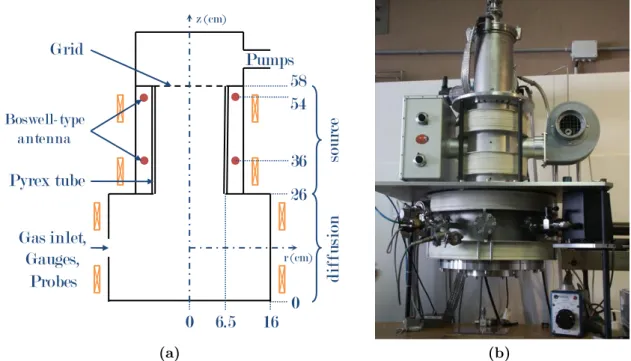
3 Experimental Setups 41 3.1 Helicon reactor . . . 41 3.2 PEGASES, Prototype I. . . 43 3.2.1 Geometry . . . 43 vvi CONTENTS
3.2.2 Source Region . . . 46
3.2.3 Additional Magnets . . . 47
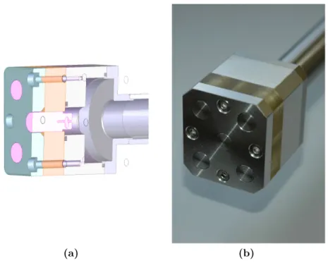
3.3 Thruster Chamber and Matchboxes . . . 47
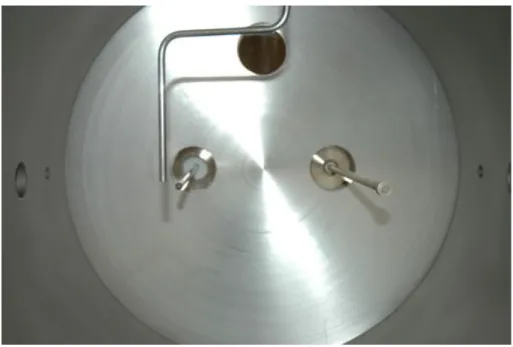
3.3.1 Thruster Chamber . . . 47
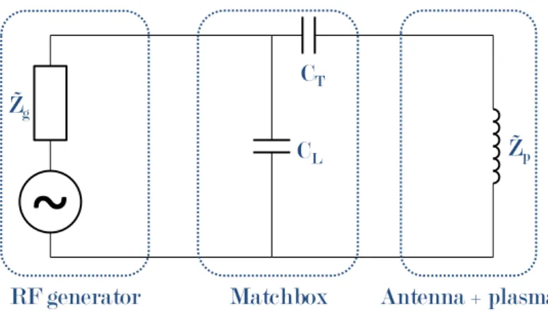
3.3.2 Matchboxes . . . 51
4 Ionization Stage 53 4.1 Power Coupling, Symmetry and Stability . . . 54
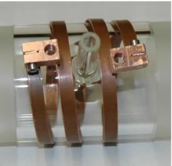
4.1.1 Helicon Mode . . . 54
4.1.2 Design Evolution . . . 55
4.1.3 Plasma Asymmetry . . . 60
4.1.4 Instabilities . . . 63
4.2 Positive Ion Current Density . . . 65
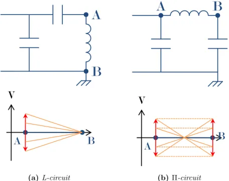
4.2.1 Original Matchbox Circuit . . . 66
4.2.2 Modified Matchbox Circuit. . . 67
4.3 Mass Efficiency . . . 70
4.3.1 Definition . . . 70
4.3.2 Non-Uniformity of the Current Density . . . 71
4.3.3 Results. . . 72
4.4 Electron Temperature . . . 72
4.4.1 Interest . . . 73
4.4.2 Discussion of the Results . . . 74
4.5 Conclusion . . . 77
4.5.1 Power Coupling . . . 77
4.5.2 Positive Ion Current Density . . . 78
4.5.3 Mass Efficiency . . . 78
4.5.4 Electron Temperature . . . 78
5 Magnetic Electron Filtering Stage - Experiments 81 5.1 Experimental Background on Ion-Ion Plasmas . . . 82
5.1.1 Ion-Ion Plasma Creation . . . 82
5.1.2 Electronegative Plasma Afterglow . . . 82
5.1.3 Magnetic Electron Filtering . . . 83
5.2 Helicon Reactor . . . 83
5.2.1 Electron Density and Positive Ion Flux . . . 83
5.2.2 I-V Characteristics . . . 86
5.2.3 Plasma and Floating Potentials, Electron Temperature . . . 89
5.2.4 RFEA Measurements . . . 92 5.2.5 Electronegativity Measurements . . . 95 5.3 PEGASES Prototype I . . . 96 5.3.1 I-V Characteristics . . . 97 5.3.2 Electronegativity Measurements . . . 97 5.4 Design Improvements . . . 100
5.4.1 Enhanced Magnetic Filtering . . . 100
5.4.2 Optimized Neutral Injection . . . 102
CONTENTS vii
II Models
105
6 Magnetic Electron Filtering Stage - Theory 107
6.1 Franklin Fluid Model in One Dimension . . . 107
6.2 Fluid Model Including End Losses . . . 110
6.2.1 Limitations of a 1D System . . . 110
6.2.2 Electron End Loss . . . 111
6.2.3 Reformulated Model with End Loss . . . 113
6.2.4 Results Using the Reformulated Model . . . 116
6.3 Analytic Approximation . . . 124
6.3.1 Analytic Model . . . 124
6.3.2 Comparison with Numerics, Parameter Scaling . . . 130
6.4 Model Limitations . . . 133
6.4.1 Symmetrical Ion-Ion Plasma . . . 133
6.4.2 Gas Electronegativity . . . 134
6.4.3 Solutions with ne(R)�= 0 . . . 135
6.4.4 Constant Te . . . 135
6.4.5 Non-Uniform Neutral Density . . . 136
7 Ion Extraction Stage 137 7.1 Description of the Problem . . . 138
7.1.1 High Voltage Sheath . . . 138
7.1.2 Low Voltage Sheath. . . 139
7.2 Basic Fluid Model Study . . . 139
7.2.1 Motivation . . . 139
7.2.2 Assumptions . . . 140
7.2.3 Poisson and Model Equations . . . 141
7.2.4 Ion-Ion Plasma . . . 147
7.3 PIC Simulations. . . 147
7.3.1 Description of the PIC Simulations . . . 147
7.3.2 Results . . . 148
7.3.3 PIC Limitations . . . 151
7.4 Kinetic Model . . . 151
7.4.1 Assumptions . . . 151
7.4.2 Initial Distribution Function Requirements . . . 153
7.4.3 Equation of the Model . . . 154
7.4.4 Bohm Criterion . . . 156
7.4.5 High Potential. . . 158
7.4.6 Floating Potential. . . 158
7.5 Conclusions . . . 162
8 Conclusions and Future Work 165 8.1 Ionization Stage . . . 165
8.2 Magnetic Electron Filtering Stage . . . 166
8.3 Extraction Stage . . . 167
8.4 Future Work. . . 167
8.4.1 What Could Not Be Done . . . 167
viii CONTENTS
A Relation Between Edge and Average Electronegativity 169
Symbols and Abbreviations
Symbol Descriptionα electronegativity (n−/ne0)
α0 electronegativity at the center (n−0/ne0)
αs electronegativity at x = R (n−(R)/ne0)
¯
α average electronegativity (¯n−/ne0)
a.m.u. atomic mass unit (1.6605×10⁻²⁷kg)
B0 static magnetic field
β normalized ion velocity at x = R (v±(R)/uB)
cs sound speed
D diffusion coefficient
e elementary charge (1.6022×10⁻¹⁹ C) ε0 vacuum permittivity (8.8542×10⁻¹² Fm−1)
f frequency
f+ positive ion distribution function
f− negative ion distribution function h positive ion edge-to-center density ratio
K reaction rate
m+ positive ion mass
m− negative ion mass me electron mass
Meff mass efficiency (Γ+/Γn|exit)
µ mobility coefficient
ν collision frequency n+ positive ion density
n− negative ion density ne electron density ng neutral density ϕ potential p pressure P power r radius
sccm standard cubic centimeters per minute T+ positive ion temperature
T− negative ion temperature Te electron temperature
uB Bohm velocity
v+ positive ion velocity
v− negative ion velocity ve electron velocity
ω angular frequency
Chapter 1
Introduction
Contents
1.1 Space Propulsion . . . 1
1.1.1 General Context . . . 1
1.1.2 Rocket Versus Electrical . . . 3
1.1.3 Electrical Propulsion . . . 6
1.1.4 Newer Concepts . . . 9
1.2 PEGASES: Plasma Propulsion with Electronegative GASES 10 1.2.1 The Idea. . . 10
1.2.2 Advantages of PEGASES . . . 13
1.2.3 Timeline and Financing . . . 13
1.3 Outline . . . 14
1.1 Space Propulsion
1.1.1 General Context
Space, or outer space, is defined as the relatively empty regions in the universe between celestial bodies. In the case of planets surrounded by an atmosphere, the latter is of course considered part of the planet and not space. It is also a region that mankind has wanted to explore for as long as Man has looked up from the ground. Contrary to the popular belief that it is a perfect vacuum, it contains atoms and particles with a density around ten per cubic centimeter [1]. For comparison, the density of air at sea level for a temperature of 20◦C is 2.5 × 10¹⁹ per cubic centimeter.
There are many reasons to send objects in space. Because of the atmosphere turbulence and city lights, observations of space are difficult and have limited accuracy. These issues can be solved by sending a telescope to space, as was the case with the Hubble Space Telescope [2]. Once in space, such a telescope can study the Earth (photos, meteorology, etc.), other celestial bodies (planets in our solar system, other solar systems, galaxies, etc.) or space itself (density of particles, radiations, etc.). An object orbiting a planet is called a satellite whether it is natural, e.g. Moon orbiting the Earth, or man-made,
2 CHAPTER 1. INTRODUCTION e.g. Hubble Space Telescope. A satellite can also be used for telecommunications: phone, television, GPS system, etc.
To achieve these objectives, a method to put the object in space and then move it, referred to as space propulsion, is needed. Any movement is described by Newton’s laws [3]:
• Every body persists in its state of being at rest or of moving uniformly straight forward, except insofar as it is compelled to change its state by force impressed, • The change of momentum of a body is proportional to the impulse impressed on the
body, and happens along the straight line on which that impulse is impressed, • For a force there is always an equal and opposite reaction: or the forces of two
bodies on each other are always equal and are directed in opposite directions. In a simpler form, these laws state that for an object to move, it has to push on another object. For instance, a pedestrian is able to walk because he is pushing on the ground with the combination of gravity keeping him on it and friction that allows him to create a force parallel to the ground. Any mean of propulsion works in the same way: cars with tires on the ground, boats with propellers on water or wind on sails, etc. As space is nearly empty (no ground to push on), these classical methods of propulsion cannot work. To solve this problem, one has to look at the third Newton law. On Earth, as an object is thrown, the thrower appears not to move. This is because the force impressed on him is transmitted to the ground through friction. In space, the sender is not held and will move in the opposite direction of the thrown object. This effect can be seen when two skaters (weak friction on the ground) push on each other and end up going away from one another. Intuitively, the faster the object is thrown, the faster the sender moves in the opposite direction. This is the principle on which space propulsion operates: a mass is accelerated and ejected from the vehicle. As a consequence, a part of the mass of the vehicle, called propellant, is used for propulsion.
Assuming that the variation of the total mass of the vehicle is negligible compared to the initial total mass M, the second Newton law can be written as
Force = Mdv
dt, (1.1)
with v the velocity of the vehicle and t time. Using the same law, the force on the vehicle T called thrust can be expressed as
T =−d
dt(mpvex), (1.2)
with mp the mass of the propellant and vexthe velocity of the ejected propellant compared to the vehicle. To simplify the problem, the exhaust velocity is assumed to be constant, resulting in
T =−vexdmp
dt . (1.3)
The mass of the spacecraft can be separated into two categories. On the one hand, the propellant which will be ejected. On the other hand, the body of the spacecraft and its cargo, also called the payload. The mass of the latter being constant,
dM dt =
dmp
1.1. SPACE PROPULSION 3 Combining (1.1), (1.3) and (1.4) yields
Mdv
dt =−vex dM
dt , (1.5)
which can be rewritten as
dv =−vexdM
M . (1.6)
For a straight line motion, this equation can be integrated from the initial state (vi, Mi)to the final state (vf, Mf). Defining ∆v = vf − vi as the increase in velocity, the integration gives
∆v = vexln Mi Mf
. (1.7)
The specific impulse Isp is defined as the ratio of the propellant exhaust velocity vex to the gravitational acceleration g [4]. Equation (1.7) can thus be rewritten as
∆v
g =Ispln Mi Mf
. (1.8)
It can be seen from this equation that there are two ways to maximize the increase in velocity: either by increasing the exhaust velocity, or the mass expelled (ratio Mi/Mf).
1.1.2 Rocket Versus Electrical
Two main propulsion methods can be used. The first is called rocket propulsion and relies on the fast expansion of a heated gas, channeled into the proper geometry. The second, electrical propulsion, consists of creating a plasma composed of ions and electrons where the ions are accelerated outward by electromagnetic forces (potential difference between two plates acting on ionic charges in the simplest case).
Rocket Engine
The heated gas for rocket propulsion can be created with a multitude of designs [5], with three as the main ones:
• chemically powered: two propellants or more, whether solid or liquid, react together to create the heated gas. One propellant is a fuel and the other one an oxidizer, • electrically powered: a monopropellant is heated electrically either directly or through
an arc,
• nuclear powered: the nuclear reaction is used to heat the propellant.
To optimize the thrust created by the heated gas, a nozzle is placed at the exit of the combustion chamber. The nozzle is the element converting most of the thermal energy into kinetic energy. The exiting gas velocity is a few kilometers per second.
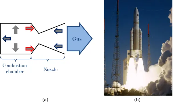
As it can be seen on figure 1.1a, the expansion of the heated gas results in pressure forces (gray arrows) on all surfaces of the combustion chamber and the nozzle. Any pressure force perpendicular to the gas exhaust does not provide thrust (no outline) as it is compensated by an opposite one. Parallel to it, a positive thrust is provided (blue
4 CHAPTER 1. INTRODUCTION
Combustion
chamber Nozzle
Gas
(a) (b)
Figure 1.1: Rocket principle(a) with the expansion of the heated gas (gray arrows): part of the pressure does not provide thrust (no outline), part does (blue outline) and part provides a negative thrust (red outline). Ariane 5 (b) combines several rocket engines to put satellites in orbit [credits Ariane Espace].
outline) when the force is opposite to the gas exhaust, and negative (red outline) when in the same direction.
Ariane 5, figure 1.1b, combines several rocket engines to take its payload from ground to orbit. Moreover, it is separated in different stages that burn one after the other. For its main core stage [6], liquid hydrogen (fuel) and liquid oxygen (oxidizer) are used as propellants, and fed in the combustion chamber with two turbo-pumps. A thrust of 1390 kN is thus provided in vacuum with a specific impulse of 432 s. As much as 170 t of propellant is ejected in 540 s.
Electrical Propulsion
A plasma is a collection of charged particles, with or without a neutral background, moving freely in a volume. In equilibrium, as electrical forces interact with the particles, a plasma is neutral on average. It is created by applying enough power to a gas to partially or fully ionize it (an atom is separated into an ion and an electron in the general case). Since only ions are used to create thrust, the process is optimized when the plasma is fully ionized: any neutral entering the chamber is turned into an ion, accelerated and provides thrust. The electrical power can either be direct-current or alternating-current. As thrusters are meant to be operated in space, the background pressure is zero. The pressure in the chamber resulting from the gas injection is thus low: plasmas in electrical thruster are low-pressure plasmas. In the case of an alternating-current electrical power, these plasmas can be created via three main modes of power coupling [7], shown in figure 1.2: capacitive (a), inductive (b) or wave heated (c).
The classical geometry of a direct-current discharge consists of a positive anode at one end and a negative cathode at the other. When the constant electric field between the
1.1. SPACE PROPULSION 5 IRF Plate Plasma (a) IRF Plasma Dielectric tube Antenna (b) IRF
Plasma Dielectrictube
Static B coils Wave launching antenna (c)
Figure 1.2: Modes for plasma creation with an alternative-current electrical power: capacitive(a), inductive (b) and wave heated(c) in the case of a helicon wave which needs a static magnetic field to be launched.
two electrodes is high enough, the neutral gas is ionized and a plasma is created. The advantage of these discharges, compared to alternating-current ones, is that all plasma parameters are constant, and thus more easily investigated. However, the structure of the discharge is quite complicated.
The simplest structure of a capacitively coupled discharge consists of two plates sur-rounding a volume where a gas is introduced. The applied power creates an electric field between the two plates. When this electric field is strong enough to ionize the neutral gas, a plasma is created. As a plasma is quasi-neutral, most of the potential difference occurs in a small region, called a sheath, near the polarized plates. The plasma density obtained is of the order of 1016 m−3. For the discharge to be considered capacitive, the characteristic length of the plates should be small compared to the vacuum wavelength of the electric field when the applied power is alternating [8]. Otherwise, a standing wave effect occurs [9] with the consequence of the induced magnetic field playing a role in the discharge equilibrium [10], as in an inductively coupled discharge.
In an inductively coupled discharge, the magnetic field induced by a current creates and sustains the plasma. The applied power is coupled to the plasma with a coil which can be either around the plasma volume or placed next to one of its containment walls. This results in the creation of an evanescent wave in the plasma. The walls of the plasma volume should be made out of dielectric material to allow the electromagnetic field to penetrate. The plasma density about 1017-1018 m−3 is higher than capacitively coupled discharges. It should be noted that in the case where the antenna is close to the wall, a capacitive coupling does occur, resulting in a simultaneous capacitive and inductive power coupling.
The last mode of power coupling is the wave heated discharge. The waves can either be created outside of the plasma, as in microwave discharges [7], or created directly in the
6 CHAPTER 1. INTRODUCTION plasma itself by another mode, such as helicon discharges [11,12]. In the case of a helicon discharge, a static magnetic field is necessary for the wave to exist in the plasma. Several helicon modes exist [13, 14] and require specifically designed antennae to be efficiently excited. The typical plasma density around 1018-1019 m−3 is higher than both previously discussed modes.
The electrical nature of the ion acceleration allows high exiting velocities, therefore a high Isp, to be reached. However, as the neutral gas is used at low pressure, the expelled mass is small. The resulting thrust is usually low with a maximum around 1 N. As an example, the Hall thruster BPT-4000 [15] at a maximum power of 4.5 kW delivers a thrust of 254 mN with an Isp of 2150 s.
Comparison
Rocket and electrical propulsion have different characteristic values: high thrust and low Isp for the first, and low thrust and high Isp for the second. Therefore, on average, they are used for different types of missions.
As a rocket engine expels a lot of propellant, it cannot be used for long term missions where the weight and volume of the stored propellant would be too large. However, it is the only method of bringing an object from ground to orbit with thrusts ranging as high as a few meganewtons.
The situation for electrical thrusters is the opposite as the thrust is very small com-pared to a rocket engine. Nevertheless for a small weight and volume of stored propellant, this low thrust can be sustained for an extended time. Electrical thrusters are well suited for long missions.
In the case of sustaining a satellite in orbit around Earth where friction forces due to the atmosphere need to be compensated, either propulsion method is reasonable since the required thrust is low and the propellant usage scarce enough for a rocket engine not to be cumbersome.
However, there is a significant drawback to electrical propulsion: the electrical power needed to operate electrical thrusters is not directly available from the power conversion systems on satellites and probes [16]. These systems convert the power collected by solar panels into usable power at given voltages and currents. Depending on the type of electrical thruster, the demand in voltage or current is too high for classical power conversion systems. An additional power conversion subsystem, therefore, is needed which adds weight to the spacecraft. As the mass of the power conversion subsystem depends on the amount of power required, an efficiency parameter is the mass to available power ratio called specific mass in kgkW−1, multiplying the classical efficiency of a power supply (ratio of delivered power to consumed power). In the case of Hall thrusters, specific masses can be as high as 10 kgkW−1 for power efficiencies as high as 93%. Again, as voltage and current requirements depend on the type of thruster, the power efficiency also depends on it: for ion thrusters, the maximum power efficiency is around 88%.
1.1.3 Electrical Propulsion
As described previously, the electrical propulsion relies on the creation of a plasma where the positive ions are accelerated and expelled to create thrust. Two main categories of electrical thrusters are currently being used for space missions: the ion thruster and the Hall thruster.
1.1. SPACE PROPULSION 7 e-
Power
Gas
Xe Xe+ Xe* e- Xe Xe+ Grids CathodeIon
beam
(a) (b)Figure 1.3: Ion thruster principle (a) with three stages: plasma creation, ion ac-celeration (grids) and neutralization (cathode). Picture of an ion thruster (b) with the exiting ion beam [credits NASA JPL].
Ion Thruster
Three stages characterize an ion thruster: plasma creation, ion acceleration and neutral-ization. These can be separated in three different regions of the thruster as can be seen schematically in figure1.3a.
The different modes possible to couple energy to a plasma were presented in sec-tion 1.1.2. The electrical power can either be direct-current or alternating-current. The aim of the first stage is to obtain a fully ionized plasma for a minimum power, with the ideal situation of every atom or molecule converted into an ion. However, an atom can also be excited without separating into an ion and an electron. The two types of reac-tions possible can be written in the case of xenon (a widely used propellant for electrical thrusters) as
Ionization : Xe + e− → Xe++ 2e− (1.9)
Excitation : Xe + e− → Xe∗+e− (1.10)
Both processes are functions of the electron energy. For Maxwellian electrons and a temperature below 8 V (9.3×10⁴ K), the excitation rate exceeds the ionization rate. This means that the ionization process is fairly inefficient for such electron temperatures. The design for the power coupling should minimize the part used for excitation by producing electron temperatures as high as possible, or non-Maxwellian distributions with enhanced tails of high energy electrons. One containment method is to employ a magnetic field cusp, using permanent magnets around the plasma volume.
Once the ions are created, they need to be accelerated, thus forming an ion beam which can be seen in figure1.3b. Although not the only possibility, the main method of ion acceleration consists of biased grids. This mechanism relies on the fact that a charged
8 CHAPTER 1. INTRODUCTION particle is accelerated in a steady electric field: potential energy is transformed into kinetic energy. A minimum of two grids is necessary: the screen grid and the acceleration grid. The role of the first grid is to ensure that no electrons enter the acceleration region where they would be accelerated back into the plasma region and damage the thruster. The potential difference between the two grids accelerates the ions outward. As grids are constantly bombarded, the choice of material is important for a long thruster lifetime: a low sputter erosion rate for the given propellant is needed. The main materials used are molybdenum, carbon-carbon composites and pyrolytic graphite. Two erosion mechanisms occur on the accelerating grid: the barrel erosion and the erosion due to secondary ions. As ions are accelerated, a part of them is collected by the accelerating grid resulting in barrel erosion: the edges of the grid holes are sputtered. At the same time, ions that left the thruster can undergo charge exchange collisions yielding a fast neutral and a slow ion called secondary ion. This slow ion, called a backscattering ion, is then accelerated toward the thruster because of the bias of the accelerating grid. A third grid positioned after the accelerating grid collects these secondary ions and preserves the accelerating grid, increasing its lifetime.
The fact that positive ions are leaving the thruster leads to a negative charging of the thruster body, which would end up in attracting the expelled ions, canceling the thrust. The exiting ion beam, therefore, needs to be neutralized, which is realized by an electron emitting hollow cathode placed at the thruster exit. There are thus two charged beams leaving the thruster, one positive and one negative. The cathode is a vital part of the thruster, and several materials and geometries are used depending on the conditions. Hall Thruster
Contrary to ion thrusters where the three stages correspond to three different regions, a Hall thruster combines all of these into one chamber. It is a gridless thruster, which, therefore, eliminates the grid lifetime issue of ion thrusters. The characteristic specific impulse is usually lower than that of ion thrusters, but the absence of current limitations due to grids makes its thrust capabilities similar to ion thrusters.
The geometry of a Hall thruster is cylindrical with its axis in the direction of the thrust, see figure 1.4a. The plasma region is annular, as can be seen in figure1.4b, and is set between an anode where the gas is introduced and a cathode at the exit of the thruster. Contrary to ion thrusters, the cathode does not only act as a neutralizer for the exiting ion beam, but is also part of the discharge mechanism. A part of the electrons emitted by the cathode feeds the channel where the plasma is created and sustained; another part flows with the exiting ion beam for charge neutrality to be fulfilled. The magnets, placed at the center and outside of the thruster body, create a radial static magnetic field. Given the mass ratio between electrons and ions, an intermediate value of the magnetic field confines the electrons (Larmor radius smaller than the system) but not the ions (Larmor radius bigger than the system). As the diffusion of electrons is impeded by the magnetic field, the potential difference between the anode and the cathode is distributed and electrons are not accelerated toward the anode. Instead, electrons have a helical motion in the channel due to the E × B drift. Ions created in the plasma are thus accelerated outward and provide thrust.
Similarly to ion thrusters, two main processes occur: ionization (1.9) and excita-tion (1.10). The aim is once again to reduce the power dissipated in excitation to op-timize the thruster. The electron temperature is higher in the channel and estimated
1.1. SPACE PROPULSION 9 Xe e- e- Xe* Xe+ B
Gas
Ion beam
Cathode Magnet (S) Magnet (N) Dielectric Anode (a) (b)
Figure 1.4: Schematics (a) of a Hall effect thruster: the plasma is created between the anode and the cathode with electrons confined along the magnetic field lines. Photo (b) of a Hall effect thruster.
around 25 V (2.9×10⁵ K), which results in a better ionization to excitation ratio.
A Hall thruster lifetime is limited by the erosion of the channel wall (dielectric) and the cathode lifetime. The material for the channel wall should have a low sputter erosion rate with the propellant, xenon in most cases. A widely used material is BNSiO2.
1.1.4 Newer Concepts
Concepts other than the ion thruster and the Hall effect thruster are being developed, but are yet to be used on actual probes or satellites. Some aim at higher power to obtain higher thrusts (VASIMIR), and others on a physical effect present in plasmas to create a gridless and anodeless thruster (HDLT).
Variable Specific Impulse Magnetoplasma Rocket
The VASIMIR thruster was invented by F R Chang-Diaz and has been in development since 1979 [17]. This thruster is composed of three stages: the plasma is first created with a radio-frequency antenna, then heated with a radio-frequency booster, and finally a magnetic nozzle transforms the energetic ions into fast moving ions.
In order to reach the highest plasma densities possible, a helicon mode of power cou-pling was chosen with as much as 30 kW delivered to the antenna. The radio-frequency booster consists of an ion cyclotron resonance: the ions are magnetized with a strong magnetic field, and an electromagnetic wave with a period equal to the period of rotation of the ions around the magnetic field lines is applied. The resulting local electric field is always in the same direction as the ion motion, accelerating the ions which end up with a high azimuthal velocity. A magnetic nozzle consists of a strong magnetic field diver-gence. As the strength of the magnetic field decreases, the azimuthal velocity of the ions
10 CHAPTER 1. INTRODUCTION is transformed into axial velocity (magnetic moment and energy conservation) [7].
The VASIMIR thruster is being tested with different propellants [18] and a recent agreement with NASA allows future tests on the International Space Station.
Helicon Double Layer Thruster
The HDLT was invented by C Charles and R W Boswell with a patent filed in 2002 [19]. As a gridless and cathodeless thruster, it removes two main lifetime limitations of thrusters. This thruster is also based on a helicon power coupling for the creation of the plasma. The radio-frequency used for the first prototype was 13.56 MHz. The set of coils creates a magnetic field not only for the helicon wave to exist in the plasma, but also provides a magnetic field divergence at the exit of the thruster. This divergence is a possible condition for the appearance of a double layer. The latter is defined [20] as two equal but oppositely charged, essentially parallel but not necessarily plane, space charge layers. The regions around it have to satisfy quasi-neutrality. The potential profile over a double layer, therefore, is an elongated step function (Poisson equation). The double layer in the HDLT appears with a negative potential difference between where the plasma is created and the thruster exit: ions going through the double layer as they diffuse are accelerated, which makes the HDLT a gridless thruster. Moreover, as the downstream plasma is quasi-neutral, there is no need for neutralization: the HDLT is a cathodeless thruster.
The main limitation of this thruster concept comes from the relatively small poten-tial difference over the double layer. As this potenpoten-tial difference is responsible for the acceleration of the ions, the specific impulse of this thruster concept is limited.
The concept of the HDLT was studied at Laboratoire de Physique des Plasmas (LPP) during Nicolas Plihon’s PhD thesis [21] in the context of an ESA report [22].
1.2 PEGASES: Plasma Propulsion with
Electronega-tive GASES
1.2.1 The Idea
The PEGASES thruster is a very recent electrical thruster concept developed in the Laboratoire de Physique des Plasmas (LPP), with a patent [23] filed in late 2005. Its principle is a consequence of studies done on a helicon reactor with electronegative gases. An electropositive gas is a gas that, in a plasma state, yields positive ions and electrons. Examples of such gases are argon (Ar), krypton (Kr) and xenon (Xe). The ionization reaction that creates the plasma can be written as
Ar + e− → Ar++ 2e−, (1.11)
for an argon plasma. The plasma equilibrium results of the interaction of two species, the positive ions and the electrons. An electronegative gas yields positive ions, negative ions and electrons. Oxygen (O2) and sulfur hexafluoride (SF6) are examples, among others. Two processes take part in the creation of the plasma: ionization and attachment. The main ionization reaction is similar to electropositive gases:
1.2. PEGASES: PLASMA PROPULSION WITH ELECTRONEGATIVE GASES 11 in the case of oxygen. The attachment reaction needs a molecular gas as electrons are too energetic to attach directly to a neutral. Part of the electron energy is absorbed by the molecule, which either breaks down into atoms and molecules or transforms the electron energy into rotational and vibrational oscillations. The breaking down reaction is called dissociative attachment:
O2+e−→ O−+O, (1.13)
for oxygen. Otherwise, it is direct attachment:
SF6+e− → SF−6, (1.14)
for sulfur hexafluoride. In the simple case of oxygen, there are three charged species that interact for the plasma equilibrium, one positively charged and two negatively charged. For bigger molecules, several species of positive ions and negative ions can be created, giving a more complex equilibrium. As a result, electronegative plasmas are prone to instabilities [24, 25, 26].
Since the power is coupled via a helicon mode, a static magnetic field is necessary and modifies the behavior of charged species as a circular motion is superimposed on their trajectories. The radius of such circular motions is called the Larmor radius and can be expressed as
rL = mv⊥
|q|B, (1.15)
with m the particle mass, v⊥ its velocity perpendicular to the magnetic field, q its charge and B the strength of the magnetic field. Comparing the Larmor radius of a species and the characteristic length of the plasma volume gives a rough indication whether it is magnetized or not. As positive and negative ions have comparable masses, there are two characteristic Larmor radii in an electronegative plasma, that of the electrons and that of the ions. The mass ratio between electrons and ions (5.8 × 10⁴ for O+
2) is such that the Larmor radius for electrons is much smaller than the one for ions. Therefore, it is possible to choose a magnetic field strength for a given characteristic dimension where electrons are magnetized but ions, both positive and negative, are not. Considering the cylindrical geometry of a helicon reactor, the electrons may be confined to the center where they are created, while ions may diffuse more rapidly across the magnetic field. An electron-free plasma, or ion-ion plasma, may be created in the periphery of the electronegative core. This is possible since quasi-neutrality can be fulfilled with two oppositely charged species. A steady-state ion-ion plasma can be created in this way.
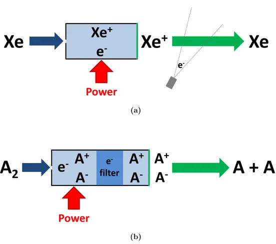
The idea behind PEGASES consists of using both positive and negative ions for thrust, contrary to classical thrusters using positive ions only as can be seen in figure 1.5a– b. The general structure of PEGASES is similar to a classical electropositive thruster: a propellant is ionized by applying electrical power and the ions are accelerated with an electrical method to create the thrust. However, there are many subtleties. First, an electronegative propellant is chosen and yields three species: positive ions, negative ions and electrons. Second, between the plasma creation and the ion acceleration is an additional stage where the electrons are filtered by a static magnetic field. Third, both ion species are accelerated to provide thrust. After different acceleration methods were considered, biased grids were chosen and will be discussed in chapter 7. Finally, there is no need for neutralization with a cathode as the accelerated beam is neutral to begin with. In order to maximize the plasma density, a helicon mode is chosen as the power coupling method.
12 CHAPTER 1. INTRODUCTION
Xe
Xe
+
Xe
+
Xe
e
-‐
e
-‐Power
(a)A
2
A
+
A + A
A
-‐
e
-‐
A
+
A
-‐
e
-‐filter
A
+
A
-‐
Power
(b)Figure 1.5: Principle of an electropositive plasma thruster (a) with xenon as pro-pellant and principle of the PEGASES thruster (b) with A2 as electronegative pro-pellant.
1.2. PEGASES: PLASMA PROPULSION WITH ELECTRONEGATIVE GASES 13
1.2.2 Advantages of PEGASES
Not only is PEGASES a revolutionary thruster concept because it uses both positive and negative ions for thrust, but it also possesses key advantages compared to classical electropositive thruster.
As described above (1.2.1), the ion beam created for the thrust is neutral, rendering a neutralizing cathode unnecessary. Therefore, the PEGASES thruster lifetime is not limited by the cathode lifetime. Compared to Hall thrusters, the elimination of the cathode ensures that no electrons are accelerated back toward the plasma chamber, which is a source of wall erosion, and a thruster breakdown possibility.
In an electropositive thruster, the process of neutralizing the ion beam with electrons should end with the recombination between these two species, but in the case of PE-GASES, the recombination happens between positive and negative ions. The velocity component of ions contributing to the thrust is along the thruster axis, with any other component either useless or deteriorating the total thrust. For optimization, the beam should be neutralized as soon as possible as a singly charged beam will diverge due to electrical forces, the same charge particles repelling one another. As the recombination between positive ions and negative ions is significantly faster than that of positive ions and electrons, a beam divergence is less likely to happen for the PEGASES thruster. For comparison in the case of oxygen, the reaction rate for the recombination between O+
2 and an electron is 2.2 × 10⁻¹⁴/ √
Te m3s−1, and for the recombination between O+2 and O−, 5.2 × 10⁻¹⁴(0.026/T
i)0.44 m3s−1. The ratio between the two constant factors of these reaction rates is 2.5. The temperature dependence further increases the ratio of ion-ion recombination to electron-ion recombination: for the typical values of Te = 3 V (3.5×10⁴ K) and T
i = 26mV (300 K), the ratio becomes 4.1. For an electron temperature of 10 V (1.2 × 10⁵ K) and the same ion temperature, the ratio is 7.5. It should be noted that the ion-ion recombination rate is even faster for other gases like sulfur hexafluoride (SF6) and dichlorine (Cl2).
When grids are used to accelerate ions, the grid lifetime is limited by erosion due to backscattering ions, described in section 1.1.3. This process is also limited by how fast ions are neutralized. Since the recombination for the PEGASES thruster should be significantly faster, the grid lifetime should be increased in the case of a PEGASES thruster using grids for ion acceleration.
1.2.3 Timeline and Financing
The PEGASES thruster project began with the filing of a patent by Pascal Chabert on December 7, 2005 [23]. This patent describes the basic idea of this new thruster concept (see 1.2.1). At that time, no experiments or modeling had been done.
I began working on this project in March, 2006, for a four month long internship which was part of my Plasma Physics Master Degree. I investigated ion-ion plasmas created in the helicon reactor and worked on the early beginning of sheath modeling for ion-ion plasmas.
I obtained a three year PhD grant in May, 2006, to begin in September, 2006. This grant was financed by Ecole Polytechnique and required me to spend a minimum of two months abroad for a collaboration. Concurrently, an ANR Jeunes Chercheurs grant was awarded to Pascal Chabert, to be used for this project. Two Post-Docs were recruited for PEGASES related work. Ane Aanesland obtained a Marie Curie grant (Europe) for a
du-14 CHAPTER 1. INTRODUCTION ration of two years on the experimental aspects of the PEGASES thruster. Albert Meige, through the ANR Jeunes Chercheurs, worked for eighteen months on PIC simulations.
The first year of the project (September 2006 - August 2007) was spent designing the first PEGASES prototype and ion-ion plasma sheath modeling with fluid models, PIC simulations and kinetic models. A group of students from Ecole Polytechnique took part in both aspects of the PEGASES project for their Projet Scientifique Commun (PSC), with two hours per week dedicated to it. I supervised two students working on the experiments and a third one on ion-ion plasma sheath modeling. A visit to Pivoine 2G, located in the ICARE laboratory, was organized. It consists of a large test chamber for thrusters where different diagnostics, among which a thrust scale, can be used to characterize a thruster model. One of the tested thrusters was the Hall thruster PPS1350-G which was chosen as the propulsion system on the Smart-1 mission coordinated by the European Space Agency. By the end of the year, the first PEGASES prototype was assembled, along with its vacuum chamber and electrical diagnostics.
During the second year (September 2007 - August 2008), the PEGASES prototype was characterized, as well as evolutions of the first design. The kinetic study of ion-ion plasma sheaths was continued. Another group of students from Ecole Polytechnique picked up where the previous one had left off: experiments on the PEGASES prototype and ion-ion plasma modeling. I once again supervised two students working on the experimental part of the project. As was required by my PhD grant, I spent ten weeks (between March and May) at UC Berkeley, California, to work with Allan J Lichtenberg and Michael A Lieberman from the Electrical Engineering and Computer Science department at UC Berkeley, on the magnetic electron filtering in electronegative plasmas to obtain an ion-ion plasma. Fluid models were developed in the case of an oxygen plasma. During this year, EADS-Astrium, a european company in space propulsion, took interest in the PEGASES thruster, bought the patent back from Ecole Polytechnique and started a collaboration with the laboratory.
The third year (September 2008 - August 2009) saw the continuation of experiments on the PEGASES prototype and further evolutions of its design. The collaboration with UC Berkeley on the magnetic electron filtering went on. On November 28, a new patent on the PEGASES thruster [27] was filed by Pascal Chabert, Ane Aanesland, Albert Meige and me. In the context of the collaboration, it was paid for by EADS-Astrium. At the start of the year, Ane Aanesland became a permanent researcher in the laboratory on the PEGASES thruster, specifically on the experimental part. Also, Lara Popellier started working in March on the experimental aspects of PEGASES during an internship, part of her Plasma Physics Master Degree. She will be picking up the work on the PEGASES project from where I left off during her PhD thesis to start in September, 2009.
1.3 Outline
First, a short background on plasma physics is presented in chapter 2, with the various models and diagnostics which were used for this thesis. The models range from PIC simulations, through kinetic models, fluid models, to global models. The notations are also defined. Two types of diagnostics were used, Langmuir-type probes and a retarding field energy analyzer. Electronegativity measurement techniques are also presented, with an emphasis on the electrostatic probe technique, used in this thesis.
1.3. OUTLINE 15 magnetic electron filtering stage, and the ion acceleration stage. These stages form the structure of this thesis, which moreover, is divided into experimental results in partI and modeling results in partII.
Ionization Stage
• In chapter 3, the different experimental setups are described: the helicon reactor, the PEGASES thruster prototype I, the vacuum chamber for the thruster, and the matchbox for the thruster.
• In chapter 4, the ionization stage in the first PEGASES prototype is investigated, with emphasis on the energy coupling, the positive ion flux, the mass efficiency, and the electron temperature profile.
Magnetic Electron Filtering Stage
• In chapter5, the experimental aspect of the magnetic electron filtering is investigated with Langmuir-type probes, a retarding field energy analyzer, and electronegativity measurements. First, in the helicon reactor in which ion-ion plasmas were originally obtained, then, in the PEGASES thruster prototype I, in which ion-ion plasmas could only be obtained after design improvements.
• In chapter 6, the fluid modeling of the magnetic electron filtering, the result of the collaboration with UC Berkeley, is presented. It consists of numerical and analytical solutions to the fluid equations of the model. The role of electron and positive ion axial losses (along the magnetic field lines) is stressed. The scaling of the main outputs (negative ion flux and thruster radius) is described as a function of the main parameters.
Extraction and Acceleration Stage
• In chapter7, the structure of sheaths in ion-ion plasmas is investigated. The problem is first treated with basic fluid models, corresponding to two extreme cases of ion-ion plasmas. The existence of a Bohm criterion-ion for ion-ion-ion-ion plasmas is then shown with PIC simulations and a kinetic model. With this Bohm criterion fulfilled in the kinetic model, two cases are studied: high voltage sheaths corresponding to a biased grid, and low voltage sheaths corresponding to the potential structure with dielectric walls (floating potential). It will be shown that the classical scaling law of the floating potential in the electron-positive ion case is woefully wrong for ion-ion plasmas.
In chapter8, the different conclusions from the work presented in this thesis are sum-marized, as well as a brief overview of the future of the PEGASES thruster project.
Chapter 2
Models and Diagnostics for Plasmas
Contents
2.1 Models for Plasmas . . . 17
2.1.1 Notations and Units . . . 17
2.1.2 The Various Models . . . 18
2.1.3 Maxwellian Species . . . 22
2.1.4 Boltzmann Relation . . . 22
2.2 Diagnostics . . . 22
2.2.1 Langmuir Probes . . . 23
2.2.2 Voltage and Current Probe . . . 29
2.2.3 Retarding Field Energy Analyzer . . . 29
2.2.4 Instruments . . . 31
2.2.5 Computer Programs . . . 33
2.3 Electronegativity Measurement Techniques . . . 34
2.3.1 Review of Techniques . . . 34
2.3.2 Electrostatic Probe . . . 36
Whether for experiments or modeling, various plasma models are needed to under-stand the plasma equilibrium. These models, as well as notations and units, are first described. The diagnostics used to characterize the plasma equilibrium in experiments are then presented. These are Langmuir-type probes, voltage and current probes, retard-ing field energy analyzer, and the various instruments and computer programs. Finally, electronegativity measurement techniques are presented, with emphasis on the one used in this thesis, the electrostatic probe.
2.1 Models for Plasmas
2.1.1 Notations and Units
General Notations
As plasmas are modeled in this thesis, three species are involved. For any variable related to one of these species, a subscript is used: (e) electrons, (+) positive ions, and (-) negative
18 CHAPTER 2. MODELS AND DIAGNOSTICS FOR PLASMAS ions.
The charge of a particle is noted q with the elementary (electron) charge e. The density n is given in m−3, the velocity v in ms−1, the flux Γ in m−2s−1, the mass m in kg.. The potential is written as ϕ in V, the electric field as E in Vm−1 and the magnetic field as B in G. For the temperature, the choice is made to use volts, with the following relation between volts and kelvins
T (K) = e kB
T (V ), (2.1)
with kBthe Boltzmann constant. It can be calculated that 1 V is equivalent to 1.16×10⁴K. The vacuum permittivity is noted as ε0.
The ionization fraction, electron density divided by the neutral density, is written as ne/ng. The ratio of negative ion density to electron density is noted as α = n−/ne. The ratio of electron to negative ion temperature is γ = Te/T−. The edge-to-center density ratio is noted h, and represents the drop in the density from the center of the plasma to the sheath edge.
Fluid Notations
The reaction rates are noted K: Kiz for ionization, Katt for attachment, Kdet for detach-ment, and Krec for ion-ion recombination. The neutral density is written as ng. Similarly, the frequencies are noted ν, with νiz = Kizng the ionization frequency for instance. In the case of collisions with neutrals, the momentum transfer rate is noted Km and the frequency ν. In the case of electrons, νe = Km,eng.
The plasma frequency of a species is noted ωp, with the following expression ωp =
� q2n ε0m
. (2.2)
As to the cyclotron frequency, it is noted ωc ωc =
qB
m . (2.3)
2.1.2 The Various Models
A plasma is a collection of charged particles (electrons and ions) and neutral particles (background neutrals and excited neutrals). Following the position and velocity of each and every particle as a function of time for all possible interactions (electric force, colli-sions, etc.) is an accurate description and its principle is similar to the N-body problem where the position of all particles is followed as a function of time with Newton’s laws. However, such a problem cannot be solved, whether analytically or numerically, due to the sheer amount of information needed: a six-dimensional vector (three for position and three for velocity) as a function of time (continuous if analytical, with a small enough time step if numerical) for all particles. For the example of a neutral gas with a pressure of 10 mTorr in a volume of 1 cm3 (very low pressure in a very small volume), there are 3.3× 10¹⁴ particles to account for, leading to 6.6 × 10¹⁴ particles for full ionization (each neutral yields an ion and an electron). Moreover, a complete description of all interactions between the particles is not feasible.
However, it is possible to use macro-particles to describe the plasma equilibrium, with each macro-particle representing a large number of real particles. These simulations are
2.1. MODELS FOR PLASMAS 19 called Particle-In-Cell (PIC) simulations [28]. The cells are defined by the mesh points and are used for the calculation of the fields on the mesh points. The macro-particles do not interact with one another with the Coulomb force, but through the fields. The collisions between macro-particles can be taken into account through Monte-Carlo simulations. PIC simulations can be used in one, two or three dimensions, but the computations, even in one dimension, are quite time-consuming. For example, the PIC simulations presented in chapter 7 were more than a week long for 2 × 10⁶ macro-particles and an average of 2000 cells.
Kinetic description
The first order of approximation is called the kinetic description. Instead of following individual particles, a distribution function for each species is considered with the position, velocity and time as function parameters: f(r, v, t). For any given (r0, v0, t0), this function returns the number of particles at the position r = r0 with the velocity v = v0 for t = t0. Using the continuity equation for the distribution function over dt, the Boltzmann equation can be obtained
∂f ∂t + v· ∇rf + F m · ∇vf = ∂f ∂t � � � � c , (2.4)
with F the sum of the forces applied on the particle. The right hand side term is called the collision term and accounts for elastic and inelastic collisional processes, among which are particle creation and loss. When it is assumed to be zero, the Boltzmann equation becomes the Vlasov equation
∂f
∂t + v· ∇rf + F
m · ∇vf = 0. (2.5)
For further simplification of equations (2.4) and (2.5), the number of dimensions can be restricted to one or two. The Vlasov equation in one dimension is written as
∂f ∂t + v ∂f ∂x + F m ∂f ∂v = 0. (2.6)
This equation is used in chapter 7 for the modeling of sheaths in ion-ion plasmas. For a characteristic sheath size smaller than the ion mean free path (distance between two collisions for ions), the collisionless assumption is justified.
Fluid description
The next order of approximation is the fluid description. Here, all quantities are the result of an integration over the velocity components of the distribution functions. A moment of order i of the distribution function f is defined as the integration of the product of this function and its argument (here velocity) to the ith power,
Mi(f )(r, t) = ���
R3
vif (r, v, t)dv. (2.7)
By definition of the distribution function, the first moment i = 0 is the density at (r, t), and the moment i = 1 is the average velocity at (r, t). To obtain relations between the vari-ables, the Boltzmann equation (2.4) is integrated using the definition of moments (2.7).
20 CHAPTER 2. MODELS AND DIAGNOSTICS FOR PLASMAS The equations are called continuity equation for i = 0 (direct integration), momentum conservation for i = 1 (integration of mvf) and energy conservation for i = 2 (integration of 1
2mv
2f). The knowledge of all the moments of a function, i.e. i ∈ N, is equivalent to the knowledge of the function. Since solving all moments of the Boltzmann equation is impossible, only a few are considered (two in most cases, sometimes three). The issue with this limited approach resides in the fact that one variable needed to solve the mo-ment of order n is solution of the momo-ment of order n + 1. For example the temperature, solution of the energy conservation, is needed to solve the momentum conservation. As-sumptions are thus needed to close the system and obtain as many variables as equations. When solving two moments of the fluid equations, the particle temperatures are usually determined by considering an additional equation, such as the power balance (described in equations (2.14) through (2.16)). In the numerical integration of the fluid model presented in chapter6, a constant electron temperature is determined by the boundary conditions. Fluid models presented in chapters 6 and 7of this thesis are one-dimensional (r = x) and steady-state (∂
dt· = 0).
The general expression of the continuity equation is
∇(nv) = G − L, (2.8)
with G the creation term and L the loss term, both of which come from the collision term in the Boltzmann equation (2.4). Ionization is an example of creation term and recombination an example of loss term. The continuity equation is thus the evolution of the flux as particles are created or lost.
An approximation of the momentum conservation equation is eT∇n � �� � pressure ± en∇ϕ � �� � E force + mnv∇v � �� � inertia + mνnv + mv(G− L) � �� � collisions = 0, (2.9)
with ± being + for positively charged particles or − for negatively charged. The pressure term uses the assumption of constant temperature as the full expression is e∇(T n). The electric force term comes from the fluid electric force ∓enE and the definition between potential and electric force E = −∂ϕ
∂x. The inertia term is the remnant part of the total derivative d dt· = � ∂ ∂t+ dx dt ∂ ∂x � · =� ∂ ∂t + v ∂ ∂x � · . (2.10)
There are two kinds of collisions taken into account. The first corresponds to collisions of the particle with background neutrals, and the second to momentum losses when particles are created or lost. This second term is usually combined with the inertia term by using equation (2.8) and yields the general expression of the momentum conservation equation
eT∇n � �� � pressure ± en∇ϕ � �� � E force + m∇(nv2) � �� � inertia + mνnv � �� � collisions = 0. (2.11)
It should be noted that m∇(nv2) is referred to as the inertia term although it is the combination of the inertia term from the total derivative and the collision term from creation and losses.
2.1. MODELS FOR PLASMAS 21 Global description
As the variables were integrated over the velocity from the kinetic to the fluid description, they are now integrated over the position to obtain the global description. Such models are often called 0D models as the dependence on the position has been removed and variables characterize the plasma in its entirety. Their goal is to relate the plasma and what is exterior to it: how the power is coupled, what happens at the walls, etc.
The plasmas considered are always enclosed in a volume, defined by surrounding walls. As a plasma is created, the electrons and ions diffuse, to be lost either in the volume (recombination for positive ions for instance) or at the walls (recombination). Due to the mass ratio, the electron diffusion is faster than that of the ions: more electrons are collected at the walls, which becomes negatively charged compared to the plasma potential. In turn, positive ions are accelerated towards the wall while electrons are confined to the center of the discharge (electropositive case). Since a plasma should be quasi-neutral, the potential difference is localized near the walls, in a region called the sheath. The complete structure is thus plasma/sheath/wall.
With a radio-frequency excitation of frequency ω, the ions cannot respond to the electromagnetic field as ω is higher than the ion plasma frequency. The plasma frequency ωp for a particle is defined as the frequency with which it responds to a perturbation, and its expression is ωp = � q2n ε0m . (2.12)
The scaling between the frequencies is
ωp+ < ω < ωpe. (2.13)
Therefore, the power is only coupled to the electrons, with a simplified power balance written as d dt � 3 2neeTeVT � = Pabs− Ploss, (2.14)
with Pabs the electrical power absorbed by the plasma, Ploss the electron power lost in the plasma and at the walls, VT the total volume of the plasma, and a 32 factor as the plasma considered is three dimensional. With ET the total energy loss per electron-ion pair created (dependent on the electron temperature), the power lost in the plasma can be written as
Ploss = ΓeAwall VT ET
(Te), (2.15)
with Γe the electron flux at the walls, and Awall the area of the walls. In a steady-state regime, the absorbed and lost power compensate one another
Pabs = Ploss. (2.16)
As the electron flux is proportional to the electron density, equations (2.15) and (2.16) mean that for a relatively constant electron temperature, the electron density is propor-tional to the applied power. It should be noted that the power balance presented here was simplified for the sake of clarity.
22 CHAPTER 2. MODELS AND DIAGNOSTICS FOR PLASMAS
2.1.3 Maxwellian Species
When a species reaches a thermodynamic equilibrium, its velocity distribution function can be expressed as a function of its temperature
f (v) = A exp−mv 2
2eT, (2.17)
with A a normalization factor, usually determined by the density with n = �Rf (v)dv. It can be seen that this expression is in fact a balance between kinetic energy (1
2mv
2) and thermal energy (eT ).
Although the considered plasmas are never in thermodynamic equilibrium, it is possible for some species to be in such an equilibrium on their own. For instance electrons are often assumed to be Maxwellian in global models and simple fluid models.
The kinetic model in chapter 7 uses Maxwellian-based distribution functions as as-sumptions to solve the Vlasov equation (2.6).
2.1.4 Boltzmann Relation
The Boltzmann relation is derived from equation (2.11) for the electrons. They are as-sumed to be massless, the inertia term is dropped, and collisionless. This equation becomes
eTe∇ne= ene∇ϕ, (2.18)
where only two terms are kept, pressure and electric force. Simplifying it yields ∇ne
ne
= ∇ϕ Te
. (2.19)
For x = 0, which usually corresponds to the center of the plasma, the electron density is set to ne0 and the potential to zero. Equation (2.19) can be integrated between 0 and x
� x 0 d(ln ne) = � x 0 dϕ Te , (2.20)
which gives the expression of the Boltzmann relation
ne(x) = ne0eϕ(x)/Te. (2.21)
With the approximation in (2.18), the electron density is only a function of the potential.
2.2 Diagnostics
Two kinds of electrical diagnostics were used to characterize the plasma: Langmuir-type probes and a retarding field analyzer. These require additional instruments and computer programs for repetitive and/or fast measurements.
2.2. DIAGNOSTICS 23 Vp Vf V I I- sat I+ sat (a) Vp Vf V I I (Vp) (b)
Figure 2.1: Sheath-free I-V characteristic (a) and actual I-V characteristic (b) for plasmas where the electrons dominate the equilibrium. The current from negative charges (electrons and negative ions) is arbitrarily chosen as positive.
2.2.1 Langmuir Probes
Principle
The idea of Langmuir-type probes consists of placing a conductor in the plasma and looking at the collected current for a given bias or range of bias. The curve of the collected current as a function of polarization voltage is called an I-V characteristic, with the arbitrary choice of plotting the electron current as positive, and the positive ion current as negative as a consequence.
The plasma potential Vp is the potential at which the plasma sets itself in regards to the surrounding walls in order to confine electrons when these dominate the plasma equilibrium. As a result, all species, regardless of their velocities, are collected by a conductor biased to this potential. The floating potential Vf is the potential for which a biased probe would collect a net current of zero. Although the net current is zero, positive (ions) and negative (electrons, negative ions) charges are collected.
In a case where temperatures are negligible for all species, an I-V characteristic would be a step function centered around Vp with I(V < Vp) = Isat+ and I(V > Vp) = Isat−. In an electron dominated plasma, however, the electron temperature is too high (∼ 3 eV) to be neglected while the ion temperatures are low. This means that an important part of the electrons have a high velocity, with the ability to overcome potential barriers. With the assumption of a Boltzmann equilibrium (see equation (2.21) in section 2.1.4), the expression of the density of electrons for a given voltage applied to a conductor is
ne(V ) = ne0e(V−Vp)/Te. (2.22)
Assuming a thermal flux for the electrons, the current is Ie= Ie0e(V−Vp)/Te with Ie0 = eAne0 ¯ v 4 = eAne0 � eTe 2πme , (2.23)
with A the area of collection. As V is decreased from Vp, the electron current is decreasing exponentially. The resulting I-V characteristic can be seen in figure 2.1a. Increasingly, as soon as V reaches Vp, all electrons are collected which is the reason why there is a
24 CHAPTER 2. MODELS AND DIAGNOSTICS FOR PLASMAS saturation for V > Vp. As V is decreased from Vp, more and more electrons are repelled, until a certain voltage where all electrons are reflected and the collected current is a pure positive ion current. During this phase, the floating potential is reached when the potential difference (Vf− Vp)reduces the electron current to the positive ion current. For smaller values of bias, the current saturates to the positive ion current.
The previous description does not take sheaths into account for the saturation currents. As the bias |V − Vp| is increased, either toward the negative or positive current, a sheath is formed between the plasma and the conductor. The size of this sheath increases with the potential difference |V − Vp|. As a consequence, the volume of the sheath region increases, which means that the collection surface (sheath surface) is increased with |V − Vp|. Therefore, there is no saturation for V > Vp or V < Vp with all electrons reflected, but an increase of absolute collected current. Although the scaling is the same for electrons and ions, this increase is more significant in the case of electron collection because of the temperature difference between electrons and ions. The resulting I-V characteristic can be seen in figure 2.1b.
An I-V characteristic can be used to obtain different plasma parameters. The first parameter is the floating potential as it can be easily determined from an I-V characteristic: I(Vf) = 0. The second parameter is the plasma potential. For V < Vp the current follows an exponential (repelled electrons) and its curvature is thus positive. For V > Vp, it is slowly increasing as a result of sheath expansion with a negative curvature. Therefore, the point I(Vp) is an inflection point and can be determined by calculating the second derivative with d2I(V
p)
dV2 = 0. The third parameter is the ion current Ii. Although there is no flat saturation current because of sheath expansion, the ion current can be determined using the Orbital Motion Limited theory [29] for a cylindrical collector which gives Ii(V )∝ �
V − Vp +const with the proportional factor depending on the probe dimensions. The fourth parameter is the electron temperature Tethat can be obtained with the assumption of Boltzmann electrons. Taking the logarithm of the electron current in (2.23) gives
ln Ie = ln Ie0+
V − Vp Te
. (2.24)
The electron temperature can thus be determined from the slope of ln Ieas a function of V . It should be noted that if the ion current is non-negligible compared to the electron current, the electron temperature is obtained from the slope of ln (I − Ii) versus V . The last parameter is the electron density, determined from the current at Vp and equation (2.23) where the expression of the average velocity ¯v is a function of the electron temperature. Since there is no sheath at V = Vp, the area of collection A is the probe area.
The situation for an ion-ion plasma differs from the electron dominated one as both species, negative and positive, have comparable masses and temperatures, usually much lower than the electron temperature in a classical electron-ion plasma. Because of sym-metry, the floating potential is zero and the saturation currents are the same: the I-V characteristic is symmetrical around the value V = Vf = 0. I-V characteristics, therefore, can be used to determine whether a plasma is electron dominated (asymmetric) or an ion-ion plasma (symmetric), as it will be discussed in chapter 5.
Radio-frequency Discharges
For a radio-frequency excited plasma, the plasma potential oscillates at the same frequency as the excitation. Harmonics, mainly the second one, can also be found. This means that