A controllably adhesive climbing robot using magnetorheological fluid

A Controllably Adhesive Climbing Robot Using

Magnetorheological Fluid

by

Nicholas Eric Wiltsie

Submitted to the Department of Mechanical Engineering

in partial fulfillment of the requirements for the degree of

Master of Science in Mechanical Engineering

at the

MASSACHUSETTS INSTITUTE OF TECHNOLOGY

MASSACHGKSFTS INST OACVESNOLOGY

T 2 22012

September 2012

@

Massachusetts Institute of Technology 2012. All rights reserved.

A uthor ...

...

.

... ...

Department of Mechanical Engineering

August 24, 2012

Certified by....

Karl Iagnemma

Principal Research Scientist, Robotic Mobility Group

Thesis Supervisor

Accepted by ...

...

...

David E. Hardt

Chairman, Department Committee on Graduate Theses

A Controllably Adhesive Climbing Robot Using

Magnetorheological Fluid

by

Nicholas Eric Wiltsie

Submitted to the Department of Mechanical Engineering on August 24, 2012, in partial fulfillment of the

requirements for the degree of

Master of Science in Mechanical Engineering

Abstract

In this thesis, the novel adhesive effects of magnetorheological fluid for use in climbing robotics were experimentally measured and compared to existing cohesive failure fluid models of yield stress adhesion. These models were found to correlate with experimental results at yield stresses below 1.12 kPa. MR fluid samples activated to have yield stresses above 1.12 kPa were limited to an adhesive stress of approximately 25-30 kPa regardless of inital fluid thickness or yield stress. A climbing robot capable of utilizing MR fluid adhesion was constructed and shown to be capable of adhering to surfaces of any orientation and climbing rough surfaces with a 450 slope. The robot was capable of controllably adhering to rough sandpaper and smooth glass with an adhesive stress of 7.3 kPa, demonstrating a novel form of adhesion on a wide range of surface roughnesses and orientations.

Thesis Supervisor: Karl lagnemma

Acknowledgments

The author gratefully acknowledges the contributions of Professors Anette Hosoi and Gareth McKinley, as well as Nadia Cheng, Ahmed Helal, Maria Telleria, and Robin Deits for their assistance in conducting these experiments and designing the robot.

This work was supported by Battelle and by the DARPA Maximum Mobility and Manipulation program.

Contents

1 INTRODUCTION

2 BACKGROUND

2.1 Magnetorheological Fluid. . . . . 2.2 Magnetic Field Strength and Flux Density . . . . 2.3 Fluid Adhesion . . . .

3 EXPERIMENTAL DESIGN

3.1 Equipm ent . . . . 3.2 Electrom agnet . . . . 3.3 Experimental Procedure . . . . 3.3.1 Fluid Thickness and Field Strength . . . . 3.3.2 Surface Properties . . . .

4 RESULTS

4.1 Critical Yield Stress . . . .

5 ROBOTIC DESIGN

5.1 Functional Requirements ....

5.2 First-Order Analysis ... 5.2.1 Robot Geometry ....

5.2.2 Magnetic Field Strength 5.2.3 Design Parameters . . . 5.3 Robot Modules . . . .

13

21

29

37

5.3.1 Magnetic Field Production . . . . 42

5.3.2 Electromagnets . . . . 42

5.3.3 Electropermanent Magnets . . . . 44

5.3.4 Permanent Magnets . . . . 45

5.4 Magnetic Field Modulation . . . . 45

5.5 Movement . . . . 48 5.6 C ontrol . . . . 50 6 Robotic Results 51 6.1 Static Adhesion . . . . 51 6.2 Climbing . . . . 54 6.3 Performance . . . . 55 7 CONCLUSIONS 57

List of Figures

2-1 Lord 132-DG MR fluid yield stress as a function of applied magnetic field intensity [1] . . . I . . . . 16 2-2 Magnetic permability curve for Lord MRF-132DG [1]. . . . . 17

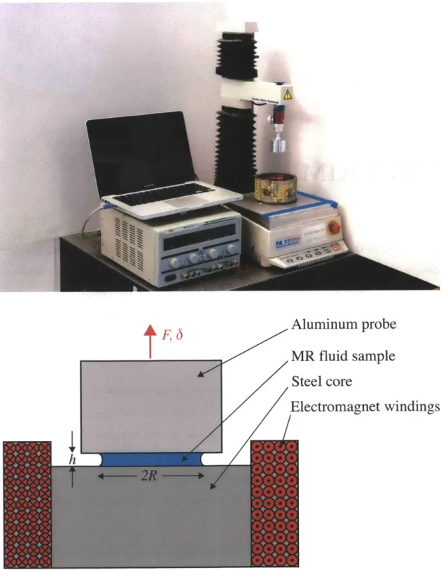
3-1 Photograph and graphic of the experimental design. A known volume of MR fluid was placed on the upper surface of the electromagnet and squeezed to a height h and radius R by the aluminum probe. The electromagnet was then activated and the two surfaces separated at a rate of 10 pm /s. . . . . 22 3-2 Finite element method magnetics simulation of the electromagnet used

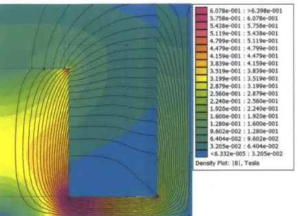
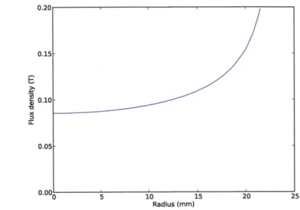
for the experiments in this study. Warmer colors correspond to higher flux densitites, and solid black lines indicate magnetic field lines. . . . 24 3-3 Example magnetic flux density along the electromagnet surface as a

function of the radius. . . . . 25

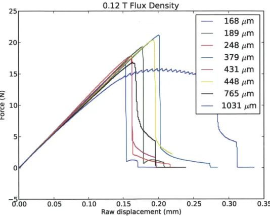
4-1 Raw force/displacement data at a flux density of 0.12 T. Image is best viewed in color. . . . . 30 4-2 Corrected force/displacement curves. . . . . 30 4-3 Peak adhesive stresses for 30mm diameter MR fluid samples at a variety

of magnetic flux densities. Samples are connected by lines as a guide to the eye. . . . . 31 4-4 Experimental data compared with a cohesive failure fluid model. . . . 32 4-5 Appearance of MR fluid samples after failure. Each sample had an

4-6 Results of the probe-tack experiments with |B| = 0.15 T. . . . .3

5-1 Geometric parameters and free body diagram of a two-footed robot. . 38

5-2 Geometric parameters and free body diagram of a two-footed robot with a spring-loaded tail. . . . . 39

5-3 An example of an amperian loop that can be used to estimate the magnetic field inside an infinite solenoid. . . . . 43 5-4 The magnetic flux produced by a 19 mm dimeter, 6 mm thick neodymium

magnet normal to planes located 0.8 mm and 32 mm away from one face. The right plot shows the flux field, where warmer colors represent higher fields and flux lines are drawn in black. . . . . 46 5-5 The permanent magnet actuation assembly. The left image is a

cross-sectional view of the robot foot, showing the two extreme positions of the magnet and the 3-D printed loop to which the cable was attached. The actuator cable entered through the tube at the top while the flex-ible sheath was press-fit around it. The right image shows the cable actuation assembly; the wire entered the tube shown in the middle and wrapped up to halfway around the spool. The front and back spool pairs were combined for spatial efficiency. . . . . 48 5-6 The path of one foot during a stepping action. The step length was

approxim ately 10 cm . . . . 49

6-1 The MR fluid-based climbing robot. . . . . 52

6-2 The robot adhering to a vertical board covered with P100 grit sanding cloth. With three of four magnets activated during a step the MRF sustained a shear of approximately 7.3 kPa; without the MR fluid, the

robot slid at an angle of approximately 450, or a stress of 0.96 kPa. . 53 6-3 The robot hanging completely inverted beneath a glass sheet. The

adhesion stress is approximately 7.3 kPa. . . . . 54 35

A-1 Corrected force/displacement curves at a flux density smooth aluminium. . . . . A-2 Corrected force/displacement curves at a flux density

smooth aluminium. . . . . A-3 Corrected force/displacement curves at a flux density

smooth aluminium. . . . . A-4 Corrected force/displacement curves at a flux density

smooth aluminium.. . . . . A-5 Corrected force/displacement curves at a flux density

smooth aluminium. . . . . A-6 Corrected force/displacement curves at a flux density

rough aluminium. . . . . of 0.03 T on of 0.06 T on of 0.09 T on of 0.12 T on of 0. 15 T on of 0.15 T on

A-7 Corrected force/displacement curves at a flux density of 0.15 T on P100 grit sandpaper. . . . . A-8 Corrected force/displacement curves at a flux density of 0.15 T on Teflon. A-9 Corrected force/displacement curves at a flux density of 0.18 T on

sm ooth aluminium. . . . . A-10 Corrected force/displacement curves at a flux density of 0.21 T on

sm ooth aluminium. . . . . A-11 Corrected force/displacement curves at a flux density of 0.24 T on

sm ooth aluminium. . . . .

61

63

63

Chapter 1

INTRODUCTION

Various methods have been developed for achieving robotic locomotion on inclined, vertical, and inverted surfaces. One of the simplest solutions for adhesion involves pressure-sensitive adhesives (PSAs) such as tape [6]. PSAs use a compliant layer of material to conform to the target surface, maximizing the contact area and creating adhesion through van der Waals forces. As van der Waals forces scale as 1/h, where h is the local separation between the material and substrate, the surfaces typically must lie within a few hundreds of nanometers of each other. PSAs can be designed to exhibit high adhesive forces but can often require relatively high forces for attachment and detachment and are subject to rapid fouling by dust and dirt.

A non-adhesive approach to enable climbing on vertical surfaces is based on the engagement of small spikes ("microspines") with surface asperities [2]. While not true adhesion, this approach enables "clinging" to surfaces with high degrees of roughness, such as stucco and brick. This technology generally cannot be employed on smooth surfaces, and can potentially damage a flexible substrate; additionally, microspines can be subject to plastic deformation and wear even under moderate loading due to high Hertzian contact stresses at the sharp spike tips.

Recently, adhesive locomotion has been achieved through the use of bio-inspired materials. Gecko lizards can achieve impressive climbing performance through the ability of their appendages to adhere to a wide variety of surfaces [3]. These ap-pendages exhibit hierarchically compliant microstructures which allow them to

con-form to rough and undulating surfaces over multiple length scales and achieve intimate contact. The van der Waals forces induced by such intimate contact produce sufficient adhesion for climbing. Moreover, gecko adhesive forces also exhibit directionality, al-lowing the gecko to adhere to surfaces with small preload forces in the normal direction and to detach with small pull-off force. However, the synthetic Gecko-like adhesives that have been developed to date are subject to fouling (like PSAs), are only effective on glass and other smooth surfaces, and are difficult to manufacture [14].

Various dry adhesives have been developed, including those based on arrays of multi-wall carbon nanotubes [27] and polymer fibers [24] [19]. These adhesives can achieve moderate levels of adhesion only with careful surface preparation and high normal preloads. Also, the size and shape of the contacting elements is important in sustaining adhesion [10] [12]. For extremely small elements such as carbon nanotubes, shape sensitivity is low, but for softer materials and larger features on the order of 100 pim the contacting element geometry dramatically affects adhesion.

The use of magnets and magnetic running gear, such as magnetic wheels and track shoes, is another common way of achieving adhesion [4] [25]. Such approaches have the obvious drawback of being effective only on ferrous substrates. Devices employing electrostatic forces have recently been developed in the context of climbing robotic systems, and have been shown to be effective on a wide variety of surface types

[26][17].

The novel form of controllable adhesion based on magnetorheological fluid ex-plored in this thesis is unique in that it can potentially be applied to a wide range of surface conditions (i.e. substrate types and roughnesses) and yield large clamping pressures without needing a ferrous substrate. This approach could potentially over-come problems with dust and other surface contaminants. One potential drawback is that fluid may be deposited on the substrate, potentially leaving evidence of the locomotion device's presence or staining the substrate with oil. Observations made during this research have shown, however, that it may be possible to recover most of the active fluid that is deposited during the adhesion process.

Chapter 2

BACKGROUND

2.1

Magnetorheological Fluid

Magnetorheological (MR) fluids are "active" or "smart" fluids composed of

micrometer-scale iron particles suspended in an inert oil. When a magnetic field is passed through a sample of MR fluid, these iron particles form microstructure chains aligned with the field direction that dramatically increase the viscosity of the MR fluid. Under suffi-cient fields this microstructure changes the fluid into a Bingham plastic, also known as a yield stress fluid, that can sustain finite stresses without flowing [18]. Yield stress fluids are commonly characterized with the Herschel-Bulkley model,

o-= -9y + Ki", (2.1)

where K and n are fit parameters describing the particular fluid [7]. For stresses

below the yield stress o-y, the fluid will behave as an elastic solid. If the fluid is forced

to yield but strained at a sufficiently low rate, i 0, it can be modelled as a perfect

plastic.

Common examples of Bingham plastics are toothpaste and peanut butter; these fluids can maintain solid forms under sufficiently low stresses (such as the body force of gravity), but will flow like a viscous fluid once a threshold stress is exceeded. A key charactereistic is that yield stress fluids will consistently transition between these

60 50 ,40

~30

Figure 2-1: Lord 132-DG MR fluid yield stress as a function of applied magnetic field intensity [1].

two states; when the applied stress is removed and flow ceases, they will again act as solids until forced to yield. Even beyond this feature of ordinary yield stress fluids, when the applied field is removed from the MR fluid it begins to acts as a Newtoninan fluid within a few milliseconds [23].

MR fluid is commonly used for applications requiring controllable viscosity or damping, such as in vehicle suspensions or earthquake vibration control systems in skyscrapers [18][22]. It has also found use as a variable damper in human interfaces

and prosthetics [11].

The yield stress of the Lord MRF-132DG MR fluid used in this study is reported graphically as a function of applied magnetic field intensity, as shown in Figure 2-1. Ewoldt et al. characterized this yield stress as increasing with the square of the applied magnetic flux,

o-, = oyO + aB 2, (2.2)

where o-yo is the small yield stress present even in the absence of a magnetic field and B is the magnetic flux density in teslas [8]. Ewoldt et al. reported these parameters as -yo ~ 6.24 Pa and a = 137737 Pa/T2

2--600 .400 -200

I4

200 400 600 500

H (kAmp/m)

Figure 2-2: Magnetic permability curve for Lord MRF-132DG [1].

2.2

Magnetic Field Strength and Flux Density

"Magnetic field" can be an ambiguous term, in that it can be used to refer to both the magnetic B-field and the magnetic H-field. These fields are related but distinct; in this thesis when the distinction is important H will be referred to as the magnetic field strength, measured in amperes per meter, and B will be referred to as the magnetic flux density, measured in teslas.

The magnetic field strength and flux density in a vacuum are related through the magnetic constant, uo = 47r - 10-7 N/A 2:

(2.3)

Nonmagnetic materials are characterized by their permeabilities are often non-dimensionalized into characteristic of the material, ,:

Po

magnetic permeability, p. These a relative permeability that is a

(2.4)

In ferrous or magnetic materials such as iron, the relationship between the field strength and the flux density is both hysteretic and non-linear; as MR fluid contains a large quantity of iron, this non-linearity can be seen in the B-H curve of the fluid's

U

a -800

datasheet included in Figure 2-2. In such cases the relative permeability becomes a function of both the applied magnetic field and the history, but for ease of calculation the incremental permeability (pA) is commonly used for first order calculations. By examining Figure 2-2, the Lord MRF-132DG fluid used in these experiments can be seen to have an initial relative permeability of pj ~ 5.97.

2.3

Fluid Adhesion

As reported by Derks et al., ordinary Newtonian fluids can exhibit a dynamic adhesive tensile or compressive force when spread in a thin layer between two parallel plates in a phenomenon known as Stefan adhesion [7]. Neglecting capillary effects and line traction, the adhesive force generated by a cylindrical drop of fluid with radius R and height h is given by the integral of the fluid gage pressure field, p(r):

R

Fadhesion = -2-x

Jp(r)rdr

0

If the fluid is confined with a sufficiently low Reynolds number and high aspect ratio, R/h

>

dh-(r2)

U(r)(27rrh)

dh r

U(r) =

r(2.7)

When Equation (2.5) is combined with the momentum balance and continuity equations for a Newtonian fluid with viscosity il, the equation for Stefan adhesion in a low Reynolds number scenario for a constant fluid volume is found as:

Fste fan =

37rR

dh

For Newtonian fluids, this effect is dependent upon the relative motion of the plates, as evidenced by the dt/dt term in Equation (2.8); with no motion, there is no pressure gradient, limiting this effect to dynamic conditions.

By contrast, yield stress fluids can sustain static adhesive and shear forces. For brevity's sake a partial derivation is shown here; Ewoldt et al. provide a full discussion of this topic [9]. A disc of yield stress fluid with radius R and height h and confined between two plates in an identical manner to the Newtonian fluid described above can be modelled as a shear-dominated lubricant. In this case any flow is shear-dominated, and at low strain rates the fluid can be modelled as a perfect plastic. By observing the force balance on an annulus of fluid, the pressure field of the yield-stress field after flow is initiated can be found as:

dp 2o-"(r)

dr h (2.9)

dr

h

In general, the yield stress may vary as a function of the fluid radius due to a non-homogenous applied magnetic field; however, the electromagnet used in these exper-iments (detailed in Section 3.2) produced a consistent field across the entirety of the fluid. If the yield stress is assumed to be constant throughout the fluid then Equation (2.9) can be integrated to find a linear pressure field, which can be combined with the force balance in Equation (2.5) to find the maximum adhesive force available from the fluid:

Fyieldstress -

2o

3h

With the yield stress characterized as in Equation (2.2), the maximum adhesive strength of a disc-shaped sample of MR fluid with radius R and thickness h exposed to a homogenous magnetic flux density B can be found to be:

FMRF= ~ y +

ozB

3 (h)

If the fluid radius exceeds that of the magnet (Rm), it is exposed to non-homogenous field intensities. Again omitting the derivation, the adhesive force for this situation

can be found to be

FMRF R -R _{( R > R,) (2.12)}

F R a> RRm

where Fm = ,7raB2R3/ho and BO is the homogenous field strength beneath the magnet.

The above analysis is focused upon tensile adhesive forces; the static shearing force that a yield stress fluid can bear is found as the simple product of the yield stress and the active area:

Chapter 3

EXPERIMENTAL DESIGN

As the goal of this research was to produce functional data to inform robotic adhesive design, the experiments focused on identifying the key parameters of MR adhesion. Specifically, these experiments were intended to identify the optimal values of the parameters that could be controlled on a mobile robot -magnetic field strength, fluid thickness, and fluid volume - as well as predict the available holding stress available based on the surface properties.

Probe tack experiments, in which a rigid steel probe is forced against an adhesive sample and slowly drawn away, are commonly used to characterize pressure-sensitive adhesives due to the ease of independently varying the adhesive area, strain rate, and initial contact force [51. Although MR fluid is not a PSA, many of the same analysis techniques can be used to characterize the nature of the adhesion, with the additional advantage that probe tack experiments, at a high level, emulate a robotic foot interacting with a target surface.

The probe tack experiments performed for this thesis were designed to investigate normal adhesion, or the force required to remove the probe perpendicularly from the target surface. Experiments measuring shear adhesion, or the force required to slide the probe along the target surface, are a topic of future work and were not conducted for this thesis.

Aluminum probe

MR fluid sample

Steel core

Electromagnet windings

h

Figure 3-1: Photograph and graphic of the experimental design. A known volume

of MR fluid was placed on the upper surface of the electromagnet and squeezed to a

height h and radius R by the aluminum probe. The electromagnet was then activated

and the two surfaces separated at a rate of 10 pm/s.

3.1

Equipment

For this thesis, a TA.XT Plus Texture Analyzer was used to perform adhesive probe-tack experiments. The texture analyzer is a linear load/displacement machine capable of applying either a specified strain rate or a sustained load to a test sample and recording the resultant force and displacement. The machine was equipped with a 5 kgf load cell with a sensitivity of ± 0.1 gf, and could report the position of the probe with a resolution of 1 pum.

A diagram of the experimental apparatus can be seen in Figure 3-1. An elec-tromagnet with a smooth-topped steel core was placed on the base of the texture analyzer, and acted as the target surface for adhesion. The robotic foot was emulated by a 43 mm diameter aluminum probe mounted to the texture analyzer's load cell through a lockable ball-and-socket joint. The relative permeability of aluminum, Iptr,

is very near to 1, ensuring that there would be a negligible magnetic force between the electromagnet and the probe.

The mating surfaces of the aluminum probe and the electromagnet (referred to hereafter as the top and bottom surfaces, respectively) were parallelized by unlocking the ball joint and slowly bringing the two surfaces into contact. As the two surfaces touched and began to load against one another, the probe was rocked from side to side to find the minimum energy state and bring the surfaces into alignment. When the load cell reported a force of approximately 1 kgf and the probe could no longer be displaced by hand, the joint was locked. The probe was slowly raised until the load cell reported a force of 10 gf, at which point the height was tared.

When loaded with an adhesive fluid sample, this system acted as a serial connec-tion of the mechanical impedances of the texture analyzer and the fluid. The texture analyzer was capable of reporting the force and position of the motor assembly at 200 Hz, but did not correct for the machine compliance. In order to reduce the com-plexity of solving for the displacement of the fluid, the linear velocity of the texture analyzer's probe was restricted to 10 pm/s. A compression test with no fluid sample (i.e. one in which the top and bottom surfaces were directly in contact) confirmed

6.078e-001 : >6.398e-001 5.758e-001 6.078e-001 5.438e-001 5.758e-001 5.119e-001 5.438e-001 4.799e-001 5.119e-001 4.479e-001 4.799e-001 4.159e-001 4.479e-001 3.839e-001 4.159e-001 3.519e-001 3.839e-001 3.1990-001: 3.519e-001 2.879e-001 : 3.1990-001 2.560e-001 2.879e-001 2.240e-001 :2.560e-001 1.920e-001 : 2.240e-001 l ll l/ ///////1.600e-001:1.920e-001 1.280e-001 : 1.600e-001 9.602e-002: 1.280e-001 6.404e-002 : 9.602e-002 3.205e-002 6.404e-002 <6.332e-005 : 3.205e-002

Density Plot: I B1, Testa

Figure 3-2: Finite element method magnetics simulation of the electromagnet used for the experiments in this study. Warmer colors correspond to higher flux densitites, and solid black lines indicate magnetic field lines.

that this test speed allowed the impedance of the machine to be well modeled as a

simple elastic stiffness of

105.72 N/m.

3.2

Electromagnet

A custom-built electromagnet powered by a benchtop power supply was used as the magnetic field source. This electromagnet consisted of 1000 turns of 21 AWG magnet wire wound around a 41 mm tall, 46 mm diameter steel core, with a steel baseplate and surrounding cylinder to help direct and concentrate the magnetic flux. The coil exhibited an electrical resistance of 14.2 Q. The coil extended 7 mm beyond the top surface of the steel core, which was flat and polished smooth, allowing for a more parallel field alignment through the MR fluid sample. A finite element method magnetics simulation of the electromagnet with a 300 pm thick MR fluid sample is shown in Figure 3-2, and a plot of the flux intensity through the middle of the sample as a function of the radius is shown in Figure 3-3.

Based on the results of these simulations, MR fluid samples were limited to a maximum radius of 15 mm in order to maintain a consistent flux density across the

E

U.

Radius (mm)

Figure 3-3: Example magnetic flux density along the electromagnet surface as a

function of the radius.

sample. These results were confirmed by measuring the flux density produced by the

electromagnet driven at several current levels with a gaussmeter. The magnet was

found to respond linearly to the applied current and produce approximately 0.06 T/A.

3.3

Experimental Procedure

3.3.1

Fluid Thickness and Field Strength

The MR fluid was prepared by vigorously agitating the fluid container for three

minutes to bring any settled iron particles into suspension. A pipette was used to

deposit a small volume of MR fluid at the center of the electromagnet. The pipette was

weighed on a Mettler Toledo XS64 analytical balance before and after fluid deposition

in order to determine the mass of the fluid sample. As the fluid's data sheet reported

a range of fluid densities between 2.98 and 3.18 g/cm

, a value of 3.00 g/cm

was

chosen to estimate the volume of the deposited fluid [1]. The necessary fluid height

to create a cylinder with a 30 mm diameter was calculated from this volume.

texture analyzer's control software. As the texture analyzer and load cell were mea-sured to have a series compliance of approximately 105.72 N/mm and the maximum force observed at this minimum thickness point was observed to be on the order of 10 gf, the positional error was less than 1 pm. No attempt was made to correct for this error. The electromagnet was energized and the experimental run started, with the plates separating at a rate of 10 pm/s and data collected at 200 Hz. The experiment was manually stopped when the the force reported by the texture analyzer dropped below 10 gf. The surfaces were then manually separated and the electromagnet deac-tivated. The maximum fluid diameter, observable by the residual stain on the bottom surface (see Figure 4-5 for an example), was measured with a pair of calipers. This diameter was used during the data analysis to compensate for any misestimation in the fluid density. The plates were then cleaned and the MR fluid discarded.

A number of trials with differing fluid thicknesses were conducted for each level of flux density, as determined by the current in the electromagnet. Due to the high wettability of the steel surface by the MR fluid, the fluid thickness for a 30 mm diameter contact patch was practically limited to be less than 900 Am.

3.3.2

Surface Properties

After the results of the experiments varying the fluid thickness and magnetic field strength described in the previous section were examined, additional experiments examining the effect of the probe's surface properties upon the adhesive stress were conducted.

Three additional surface types were tested in addition to the smooth aluminum probe used in the previous experiments. First, the probe was roughened using P100 grit sandpaper. Second, the P100 sandpaper was affixed to the probe surface with epoxy. Finally, the sandpaper was removed and a smooth Teflon disk was affixed to the probe surface. The surface roughness and material type of each testing condtion is presented in Table 3.1.

For each of these three additional surface conditions, the experimental procedure described in the previous section was carried out. The magnetic flux density was fixed

Table 3.1: Surface roughnesses of experimental probes.

Material

_{Rq (PM)}

at 0.15 T, as the adhesive saturation described in Chapter 4 indicated a minimal effect of additional field strength beyond this point.

Chapter 4

RESULTS

An example of the raw force/displacement data collected across a range of initial fluid thicknesses at a magnetic flux density of 0.12 T is shown in Figure 4-1. The displacements shown in these plots are of the machine-fluid system; in order to extract the fluid displacement, the stiffness of the texture analyzer found in Section 3.1 was subtracted from the total displacement:

6totaI = 6fIuid + 6 TA (4.1)

oTA

(4.2)

Two examples of the resulting force/corrected displacement curves can be seen in Figure 4-2. The remainder of these plots are presented in Appendix A. The data in Figure 4-2a were collected at "low" fields of 0.03 T, while the data in Figure 4-2b were collected at "high" fields of 0.21 T. From these plots it is apparent that the fluid deforms relatively little before failing, regardless of the flux density. However, the deformation path after failure varies greatly between the two plots; at low fields the fluid exhibits substantial ductility, while at high fields it behaves very much like a brittle solid. In order to more fully examine the effect of fluid thickness and flux density upon the failure modes of the fluid samples, the peak force of each sample was

0.12 T Flux Density

379 pum

765 pm

Figure 4-1: Raw force/displacement data at a flux density of 0.12 T. Image is best viewed in color. 0.03 T Flux Density , - 34pm 6 - 57 pm - 125 pm 5 - 166 pm - 170 pm 4 212 pm - 268 pm 3 - 342 pm - 429 pm 2 - 538 pm - 615pm 0 '1 0.0 0.1 0.2 0.3 0.4 Corrected displacement (mm) (a)

IBI

Figure 4-2: Corrected force/displacement curves.

201-15 10 z L-u* 5 0

(.0 o

Peak Engineering Stress

0.03 T

->-+

0.09 T

Initial fluid thickness (pm)

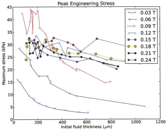
Figure 4-3: Peak adhesive stresses for 30mm diameter MR fluid samples at a variety

of magnetic flux densities. Samples are connected by lines as a guide to the eye.

extracted and normalized by the measured contact area into an engineering stress.

The MR fluid adhesion stress is plotted as a function of initial fluid thickness,

organized by magnetic flux density, in Figure 4-3. From this plot it is apparent

that there are two distinct failure mechanisms in operation: at low flux densities the

adhesive stress is inversely proportional to the fluid thickness, but between 0.09 T

and 0.12 T the adhesive stress saturates. Increasing the flux density beyond this

point has very little (or even a detrimental) effect upon the adhesive stress, and the

initial fluid thickness becomes irrelevant. 0.09 T and 0.12 T correspond to fluid yield

stresses of 1.12 kPa and 1.98 kPa, respectively.

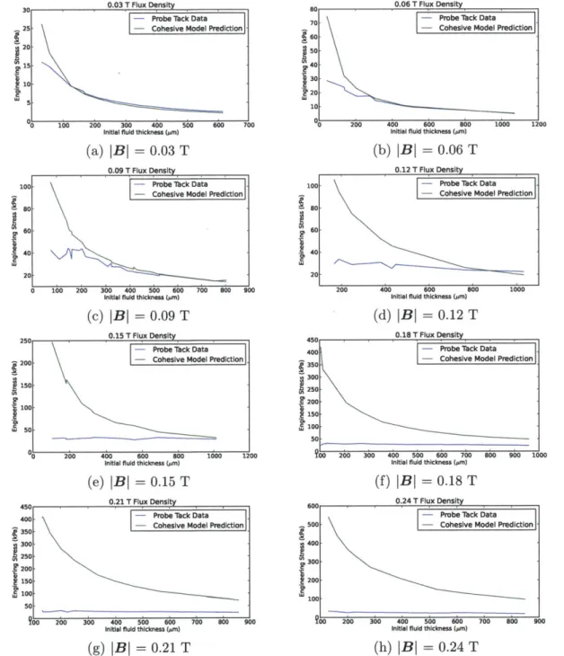
Comparison plots of these maximum stresses compared with the cohesive failure

model given in Equation (2.11) are presented in Figure 4-4. For flux densities less

than or equal to 0.09 T, the cohesive model closely corresponds to the experimental

0.03 T Flux Density -Probe ack Data

25 - Cohesive Model Prediction

20 15

10-00, 100 200 300 400 500 600 700

initial fluid thickness (sm) (a) |BI = 0.03 T

0.09 T Flux Density 100 - Probe Tck Data

- Coeive Model Prediction

80

60

40-

20-0 100 200 300 400 500 600 700 800 900

initial fluid thickness (sm) (c) |BI = 0.09 T 7Kn 0.15 T Flux Density 200 150 100 50 0 450 400 350 300 250 200 j 150 100 50 -4 Probe 8ck Data1 -Cohesive Model Predietion

1 200 400 600 800 1000

Initial fluid thickness (sm)

(e) |BI = 0.15 T 0.21 T Flux Density 70 6e0 50 40 f30 20 10 100 80 60 40 2C 400 350 300 250 200

15

-Cohesive Model Predietion

00 200 300 400 500 500 700 Boo 900

Initial fluid thickness (pm)

(g) |BI = 0.21 T

0.06 T Flux Density

2- Probe 80ck Data -Cohesive Model Prediction

17 200 400 600 800 1000 121 Initial fluid thickness (prn)

(b) |BI = 0.06 T

0.12 T Flux Density

Probe ack Data Cohesive Model Prediction

200 400 600 Bo0o

initial fluid thickness (sm)

(d) |BI = 0.12 T

0.18 T Flux Density

1000

-

Cohesive Model Prediction

-0 0 0 0 0 60 70 80 90 1

?00 200 300 400 500 600 700 S00 900 10

Initial fluid thickness (sm)

(f) |BI = 0.18 T

0.24 T Flux Density

-Probe ack Data

0 - Cohesive Model Prediction

0

0

10 0 0 0

300 400 500 6W0 7 0

Initial fluid thickness (sm)

(h) |BI = 0.24 T

0

a00 90

Figure 4-4: Experimental data compared with a cohesive failure fluid model.

I

I

,

,

,

data, with the exception of samples less than 100 pin thick. Above this critical flux density, the cohesive model greatly over-predicts the available adhesive force.

The activation of the new failure mode with increasing fluid yield stress implies that it is an adhesive, rather than a cohesive, failure. As noted in Section 2.3, the cohesive model was predecated upon the no-slip fluid assumption; that is, the fluid would remain in contact with the target surfaces and fail by yielding and flowing within the bulk of the fluid. At magnetic flux densities of 0.12 T and above, cor-responding to fluid yield stresses above 1.98 kPa, the observed maximum adhesive stress saturates. This strongly implies that failure occurs at the fluid-solid interface and not within the bulk of the fluid; the energy required to create new surfaces is independent of the fluid thickness and yield stress, and therefore once the critical fluid yield stress is exceeded the failure will always be at the interface rather than in the bulk.

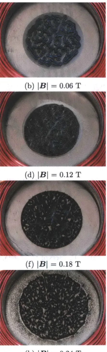
The existance of this adhesive failure mode is further supported by observation of the MR fluid samples after failure. Photographs of fluid samples after experimental runs at each of the magnetic flux levels are shown in Figure 4-5. The electromagnet remained energized through the duration of these photographs. Figures 4-5a, 4-5b, and 4-5c correspond to the magnetic flux densities that correlate well with the cohesive model. In each of these examples the bulk of the fluid moved radially inward from the original boundary, shown by the dark gray circular stain on the electromagnet surface. The results shown in Figure 4-2a indicate that this flow occured during the ductile phase after the maximum stress was achieved, showing that the fluid-solid interface remained intact while the fluid yielded internally. This response is in line with the assumptions made during the derivation of the cohesive model.

By contrast, those fluid samples which exhibited the saturated adhesive stress did not withdraw from the original fluid boundary (Figures 4-5d through 4-5h) or exhibit any ductility after the initial failure (Figure 4-2b). The lack of flow implies that the failure was at the interface, deviating from the assumptions made in deriving the cohesive failure model.

(a) IBl = 0.03 T

(c) |BI = 0.09 T (d) IBl = 0.12 T

(e) IBl = 0.15 T (f) |BI = 0.18 T

(g) |Bl = 0.21 T (h) |B| = 0.24 T

Figure 4-5: Appearance of MR fluid samples after failure. Each sample had an initial

thickness of 400 pLm and diameter of 30 mm.

Peak Engineering Stress

400 600 800

Initial fluid thickness (pm)

Figure 4-6: Results of the probe-tack experiments with |BI

=

0.15 T.

4.1

Critical Yield Stress

The critical yield stress dividing cohesive failure from adhesive failure is of paramount

importance from an engineering perspective; it sets the boundary of the maximum

adhesive stress that can be obtained from a given sample of MR fluid, as well as

defining point at which increasing flux density will cease returning increased adhesive

stress.

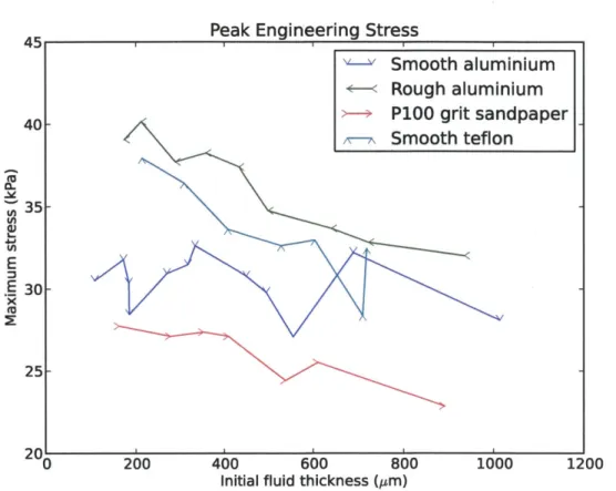
The results of the experiments in using the different probe materials given in

Table 3.1 are shown in Figure 4-6. While the maximum yield stress of the rough

surfaces varies more with initial thickness as compared to the smooth aluminium,

that variation is far less than the 1/h relation predicted by Equation (2.11). This can

be seen by comparing these results with those in Figure 4-4e

-

the cohesive model

predictions are clearly far higher than the observed stresses.

40 V--v

Smooth aluminium

Rough aluminium

P100 grit sandpaper

a

Smooth teflon

35-

While a full investigation into modelling this failure mechanism is beyond the scope of this thesis, these experiments have revealed two key points. First, the roughness of the target surface varied by two orders of magnitude between the smooth aluminium and sandpaper, but the adhesive stress varied non-monotonically and declined less than 50%. Second, the surface material varied between aluminium and Teflon with no appreciable change in adhesive stress. From an engineering perspective, this increases the attractiveness of the adhesive; the available force only varies a small amount in response to different surface types and finishes. This can be contrasted with many other robotic adhesion schemes, such as dry adhesives or microspines, which require carefully cleaned surfaces or a specific feature size.

Chapter 5

ROBOTIC DESIGN

5.1

Functional Requirements

The goal of this research was to produce a prototype mobile robot that could demon-strate MR fluid adhesion. Initial design concepts for robotic adhesion exploiting MR fluid adhesion focused on a small, low-profile, legged robot. Legged locomotion was chosen for the simplicity of adhesion events; during a step cycle each foot would contact the surface, adhere, bear a load, detach, and advance. This "discontinuous" approach was deemed more conducive to analysis of the limitations of MR adhesion than a "continuous" approach, such as a tank with an adhesive tread, despite being more mechanically complex.

An important initial design decision was to not include any mechanism for fluid dispensation onboard the robot. This greatly simplified the functional requirements of the robot, in that it did not need to account for any pumping mechanism or carry a fluid reservoir, at the expense of a much less capable robot.

At a high level, the robot was required to exploit two distinct MR fluid adhe-sion phenomena: normal adheadhe-sion, as examined through the experiments detailed in Chapter 3 and necessary while clinging to ceilings, and shear adhesion, necessary to climb walls. This would be accomplished using legged locomotion and assuming samples of MR fluid would be pre-placed or placed as necessary on the target surface by an outside observer.

Fi~y

A \

h-m

L

mg

Figure 5-1: Geometric parameters and free body diagram of a two-footed robot.

5.2

First-Order Analysis

5.2.1

Robot Geometry

A two-legged robot with mass m, center of mass height h, adhesion area per foot A,

and length between adhesive centers of pressure L is shown schematically in Figure 5-1

using MR fluid to adhere to a vertical wall. The reaction forces on the robot's feet are

drawn such that positive forces correspond to adhesion. A moment balance centered

around the center of pressure of the bottom foot reveals the necessary adhesive stress

for the single top foot to prevent the robot from falling backward due to gravity:

E(M =)2

mgh

-

F

,-L

=

0

(5.1)

mgh (5.2)

('ad)req = AL

As there are only two forces in the horizontal direction in Figure 5-1, it is clear that

this adhesive force of the front feet balancing the gravitational moment is balanced

{

mg

M---+F2y

g

z

Figure 5-2: Geometric parameters and free body diagram of a two-footed robot with

a spring-loaded tail.

by a compressive force on the hind feet.

EFx = Fi,x +

= 0

(5.3)

F1,X

-F2,

(5.4)

This force balance is inefficient, as the adhesive potential of the hind feet is wasted,

and can lead to problems with the front feet "walking off the wall". However, by

adding a spring-loaded tail that presses against the wall at a distance Ltaii behind

the rear feet with force Fta,,,x, the adhesive load on the front feet can be reduced at

the expense of the compressive force on the hind feet. This situation is illustrated

in Figure 5-2, where the the tail's reaction force is drawn such that a positive force

corresponds to compression against the wall.

E (Mz 2=

mgh

F1,xl

(5.5)

F1 =

(5.6)

E(M,)= mgh + F2,,L - Ftaui,w(L + Ltai) =0 (5.7)

mgh Ftaii,x(L + Ltaii)

(5.8)

L L

If the tail force is tuned to equalized the adhesive load between the fore and hind

feet, that force can be found as:

F1X= 2,x-+ Ftaii,x = 2mgh (5-9)

2Ltaii + L 2mgh F1,X = F2,x = mh(5.10)

2Ltai + L

The minimum necessary adhesive stress for a single front and single back foot is therefore:

mgh

(Oad)req = A(2Ltaii + L) (5.11)

While using a tail in this manner increases the total adhesive force necessary for the robot, it reduces the individual contribution from any single foot or set of feet. This enables the use of smaller feet or less powerful magnets, at the expense of additional body length necessary for the tail's operation.

5.2.2

Magnetic Field Strength

A force balance in the vertical direction sets a minimum bound on the adhesive area

and the yield stress of the MR fluid, oy:

EF = En_1(F ,y) - mg = 0 (5.12)

1(F=,y) mg (5.13)

This can be combined with Equation (2.2) to find the minimum magnetic flux neces-sary through the bulk of the fluid:

2 mg

UyO + aB 2 _{nA (5.15)}

Breq= _anA mg a- o _a (5.16 )

In a similar analysis to that of Equation (5.14), the minimum adhesive stress necessary for adhesion to a fully inverted surface can be found as

mg

(Uad)req -

A

(5.17)

nA

5.2.3

Design Parameters

Equations (5.10), (5.16), and (5.17) reveal the ideal shape of a robot using MR fluid for adhesion: a small aspect ratio (L > h), low mass, and large adhesion area will reduce the adhesive stress necessary for operation. High levels of applied magnetic flux will increase both the shear and the adhesive stress, increasing the payload capacity and reducing the necessary adhesive area.

The maximum adhesive area per foot and off-state magnetic flux are bounded by Stefan adhesion and performance requirements; as shown in Equation (2.8), the force required to remove a deactivated foot scales linearly with area, removal velocity, and fluid viscosity. As minimizing actuator mass and maximizing robot speed is desirable, the adhesive area and off-state fluid viscosity should not be arbitrarily increased beyond what is necessary for adhesion.

From Figures 4-3 and 4-6 it was determined that 25 kPa was a reasonable average value for the maximum failure stress of MR fluid activated by a field of 0.4 T across a wide range of potential surfaces. A safety factor of 2.5 reduced the expected working stress to 10 kPa.

From this value, a robot with an overall maximum footprint of approximately 30 cm by 30 cm with a total mass less than 1 kg and total adhesive area of 100 cm2 _was

production. Ultimately a four-legged walking design was chosen, with two additional fixed outrigger legs for stability and a spring-loaded tail to counteract the gravitational peeling moment while climbing. A treaded tank-style design was also considered but rejected due to the problem of sufficiently tensioning the tread to prevent separation from the main body during inverted driving.

5.3

Robot Modules

The design is easily broken into three distinct modules: magnetic field production, magnetic field modulation, and movement.

5.3.1

Magnetic Field Production

In order to control the adhesive force of the robotic feet to properly adhere and detach, it is necessary to modulate the magnetic field strength applied to the MR fluid. As observed by Lira et al., magnetorheological fluid adhesion is strongest when the magnetic field lines are aligned normal to the fluid thickness

[15].

5.3.2

Electromagnets

Electromagnets are composed of tightly packed coils of current-carrying wire that generate a magnetic field through the motion of the electrical charges. The use of electromagnets to produce magnetic fields is desirable due to their solid-state con-struction; they have no moving parts, and the field strength is modulated by altering the current. This allows for relative mechanical simplicity at the cost of increased electrical complexity.

The primary disadvantage of electromagnets in the context of an adhesive climbing robot is power consumption; the electromagnet requires continuous power to produce continuous magnetic fields. A first-order estimate for the minimal power consumption necessary for adhesion can be found from Ampere's law, which states that the line

B

t _N

Figure 5-3: An example of an amperian loop that can be used to estimate the magnetic

field inside an infinite solenoid.

integral of the magnetic B-field around a closed curve is proportional to the total current passing through the enclosed surface. This is expressed symbolically as

B - dl = poIen, (5.18)

where yo is the magnetic constant, defined to be equal to 47r -10-7N/A 2.

The magnitude of the B-field inside an infinite ideal solenoid (a straight cylindri-cal electromagnet) carrying current I can be found by choosing the amperian loop enclosing N turns shown in Figure 5-3. The only segment of this curve for which the

B - dl is non-zero is inside the coil; thus, Equation (5.18) becomes

B = (5.19)

Combining this result with the minimum necessary flux density for adhesion given

by Equation (5.16) and rearranging terms yields the minimum necessary number of

amp-turns:

NI= -

mg

y o anA a

Combining Equation (5.20) with the physical constants given in Section background

and the first-order assumptions of a 1 kg robot with a total adhesive area of 100 cm2

for a small and mobile robot.

5.3.3

Electropermanent Magnets

Electropermanent magnets combine the solid-state construction of electromagnets with the zero-power operation of permanent magnets. In their simplest form they are composed of a parallel configuration of two permanent magnets made from different materials enclosed inside an electromagnet. If the materials are well matched to have similar remnant flux densities but very different coercivities, then appropriately powered pulses of current through the electromagnet will reverse the polarity of the easily coerced material while leaving the other unchanged.

When the two magnets are aligned, the flux lines will exit the magnet assembly and can be routed with appropriate iron poles. When the magnets are opposed, due to their similar remnant flux densities the field will remain entirely within and between the magnets, leaving nothing to exit the poles. This creates an electrically switchable solid-state magnet that requires zero power to remain either "on" or "off." The disadvantages of working with electropermanent magnets are the switch-ing energy and the morphology. The energy to switch the magnet's state scales with the volume of magnetic material, or with the cube of the characteristic length. Additionally, electropermanent magnets are usually designed with nearly-complete low-magnetic-impedance circuits in order to concentrate the flux through the highly coercive magnet while minimizing power consumption. This low-magnetic-impedance requirement usually restricts the shape of the device to a horse shoe with keeper bar or nearly complete circle. To adhere via magnetorheological fluid, the horse shoe shape must be used; unfortunately, this arranges the magnetic field lines parallel to the MR fluid in an ineffecient arrangement [15].

An excellent design guide for electropermanent magnets is presented by Knaian [13]. A hypothetical device with a core consisting of two 12 mm long, 12 mm diameter cylindrical magnets with 200 turns of 26 AWG wire would have a total diameter of 31 mm. This device would require a 2 ms pulse of 18 A to change states - an event that would consume approximately 1 J of energy and require discharging a 1000 pF

capacitor charged to 50 V across the electromagnet's coils. The power electronics and capacitor mass required to manage this switching were deemed unacceptable for a mobile robot.

5.3.4

Permanent Magnets

Permanent magnets require zero power to produce strong magnetic fields; rare earth magnets can produce flux densities higher than 1 T in a smaller volume than what an electromagnet would require, and with a correspondingly smaller mass [16].

The disadvantage of working with permanent magnets is that physical distance is the primary method of modulating the flux density. The magnets must either be mechanically actuated to bring them closer or further from the target surface, or the flux must be shunted away with an external magnetic circuit.

For the purposes of this climbing robot, the advantage of the high ratio of flux density to mass expressed by permanent magnets was deemed to outweigh the me-chanical complexity of actuation. Meme-chanically actuated permanent magnets were chosen as the magnetic field sources for the climbing robot.

5.4

Magnetic Field Modulation

For a given permanent magnet interacting with a sample of MR fluid, there are two ways to alter the activation of the fluid: the field intensity may be changed by physically displacing the magnet or shunting the field, or the field direction may be changed by rotating the magnet.

At first glance the latter option seems more attractive, particularly given that spherical and non-axially magnetized cylindrical magnets exist; the magnet and the iron in the MR fluid are attracted, and there can be a substantial force acting to draw the two together. Displacing the magnet requires moving it directly away from the MR fluid, requiring relatively high forces and a large energy input. By contrast, a spherical magnet rotating in place could continually bear this force against a fixed surface while greatly reducing the flux intensity by the motion of its poles. Unfortunately,

0.5 0.4 0.3 4 0.2 0.8mm 0.1 - - - 30mm 0 0 5 10 15 20 Radius (mm)

Figure 5-4: The magnetic flux produced by a 19 mm dimeter, 6 mm thick neodymium magnet normal to planes located 0.8 mm and 32 mm away from one face. The right plot shows the flux field, where warmer colors represent higher fields and flux lines

are drawn in black.

the relative permeability of MR fluid sufficiently changes the local field shape as to make this approach ineffective; the field intensity along the "equator" of the 12 mm spherical magnets used to test this scheme was sufficient to activate the fluid.

As magnetic field intensity drops off as 1/r 3, the magnet should have as much

surface area in close proximity to the target as possible, while remaining as light as possible to reduce the load the robot must carry [21]. Given that the magnetic field intensity must be modulated by physical separation, the ideal magnet shape for maximum adhesion becomes clear: an axially symmetric magnet, such as a disc or cylinder, that is sufficiently thick to produce the required magnetic field at its face.

The magnets chosen for use were composed of grade N52 neodymium (NdFeB), shaped into discs measuring 19 mm in diameter and 6 mm in thickness.

As seen in Figure 5-4, at a distance of 0.8 mm from the magnet's face the magnetic flex density varies between 0.35 T and 0.5 T between the magnet's center and a radius of 11 mm, with a weaker field extending some distance beyond this. From Figure 4-3 it can be seen that the existence of this flux density through the robot's soles will grant a measure of freedom in fluid thickness; fluid thicknesses between 150 and 800 Pm all have similar failure stresses, suggesting that it may not be necessary to carefully

control the foot's position relative to the wall. At a distance of 32 mm from the magnet's face, the flux density drops to 0.01 T. Thus, an actuation method capable of translating the magnet between 0.8 mm and 32 mm away from the target surface would be sufficient to fully activate and fully deactivate the adhesive effect.

The robotic foot shown in Figure 5-5 was capable of actuating the magnet between these "on" and "off" states. The foot was composed of two plastic halves, joined by nylon screws: the bottom half was made from machined Delrin for mechanical strength and the top half was 3D-printed. The magnet was epoxyed to a plastic guideblock and inserted into a cylindrical cavity enclosed by the foot halves. This cavity extended from 0.8 mm above the foot's sole to the top of the foot, allowing the magnet the required translation for fluid activation and deactivation.

The plastic guideblock epoxyed to the magnet served two purposes: it prevented the relatively wide and thin magnet from jamming in the cylindrical pathway, and contained a semi-circular attachment pathway for an 24 AWG spring steel actuation wire. The wire entered the cavity through a small hole at the top of the foot, and connected to the block-magnet assembly. By feeding wire into or extracting it from the foot, the magnet could be pushed closer to the sole or pulled up to 32 mm away. The wire was sufficiently thick to bear the weight of the magnet and guideblock without buckling if the foot were inverted - as it would be if the robot were walking on the ceiling.

In order to reduce the foot's mass, and therefore the size of the actuators required to lift and move the leg during walking, the magnet's actuator was placed on the body of the robot. A rigid linkage connecting the remote actuator to the magnet would interfere with the motion of the foot unless it was very carefully designed; in order to eliminate this problem entirely, the magnet was actuated using a Bowden cable, also known as a push/pull cable.

The wire that connected to the magnet traveled within a flexible but inextensible sheath that joined the foot and the body. On the body, the wire connected to a cylindrical horn on a Hitec HS-485HB servomotor; this horn was surrounded by a co-axial cylindrical wire guide, both of which were constructed via 3D-printing. When