HAL Id: hal-02042526
https://hal.inria.fr/hal-02042526v2
Submitted on 20 Feb 2019HAL is a multi-disciplinary open access
archive for the deposit and dissemination of sci-entific research documents, whether they are pub-lished or not. The documents may come from teaching and research institutions in France or abroad, or from public or private research centers.
L’archive ouverte pluridisciplinaire HAL, est destinée au dépôt et à la diffusion de documents scientifiques de niveau recherche, publiés ou non, émanant des établissements d’enseignement et de recherche français ou étrangers, des laboratoires publics ou privés.
Fluid-attenuated inversion recovery MRI synthesis from
multisequence MRI using three-dimensional fully
convolutional networks for multiple sclerosis
Wen Wei, Emilie Poirion, Benedetta Bodini, Stanley Durrleman, Olivier
Colliot, Bruno Stankoff, Nicholas Ayache
To cite this version:
Wen Wei, Emilie Poirion, Benedetta Bodini, Stanley Durrleman, Olivier Colliot, et al.. Fluid-attenuated inversion recovery MRI synthesis from multisequence MRI using three-dimensional fully convolutional networks for multiple sclerosis. Journal of Medical Imaging, SPIE Digital Library, 2019, 6 (01), �10.1117/1.JMI.6.1.014005�. �hal-02042526v2�
Fluid-attenuated inversion recovery MRI synthesis from
multisequence MRI using three-dimensional fully convolutional
networks for multiple sclerosis
Wen Weia,b,c,*, Emilie Poirionb, Benedetta Bodinib, Stanley Durrlemanb,c, Olivier Colliotb,c, Bruno Stankoffb, Nicholas Ayachea
aUniversit´e Cˆote d’Azur, Inria, Epione project-team, Sophia Antipolis, France
bSorbonne Universit´e, Inserm, CNRS, Institut du cerveau et la moelle (ICM), AP-HP-Hˆopital Piti´e-Salpˆetri`ere,
Boulevard de l’hˆopital, Paris, France
cInria, Aramis project-team, Paris, France
Abstract. Multiple sclerosis (MS) is a white matter (WM) disease characterized by the formation of WM lesions, which can be visualized by magnetic resonance imaging (MRI). The fluid-attenuated inversion recovery (FLAIR) MRI pulse sequence is used clinically and in research for the detection of WM lesions. However, in clinical settings, some MRI pulse sequences can be missing because of various constraints. We propose to use 3D fully convolutional neural networks to predict FLAIR pulse sequences from other MRI pulse sequences. In addition, we evaluate the contribution of each input pulse sequence with a pulse-sequence-specific saliency map. Our approach is tested on a real multiple sclerosis image dataset and evaluated by comparing our approach to other methods and by assessing the lesion contrast in the synthetic FLAIR pulse sequence. Both the qualitative and quantitative results show that our method is competitive for FLAIR synthesis.
Keywords: MR Images, FLAIR Synthesis, 3D Fully Convolutional Networks, Multiple Sclerosis, Deep Learning. *Wen Wei, [email protected]
1 Introduction
Multiple sclerosis (MS) is a demyelinating and inflammatory disease of the central nervous system
and a major cause of disability in young adults.1 MS has been characterized as a white matter
(WM) disease with the formation of WM lesions, which can be visualized by magnetic resonance
imaging (MRI).2,3 The fluid-attenuated inversion recovery (FLAIR) MRI pulse sequence is
com-monly used clinically and in research for the detection of WM lesions which appear hyperintense
compared to the normal appearing WM tissue (NAWM). Moreover, the suppression of the
ventric-ular signal, characteristic of the FLAIR images, allows an improved visualization of the
periven-tricular MS lesions,4and can also suppress any artifacts created by CSF. In addition, the decrease
Fig 1: MRI pulse sequences usually used in a clinical setting.
T1-w provides an anatomical reference and T2-w is used for WM lesions visualization. However, on the T2-w, periventricular lesions are often indistinguishable from the adjacent cerebrospinal fluid (CSF) which is also of high signal. WM lesions (red rectangles) characteristic of MS are best seen on FLAIR pulse sequence because of the suppression of the ventricular signal. Double inversion recovery (DIR) has direct application in MS for evaluating cortical pathology. Proton density (PD) and T1 spin-echo (T1SE) are also used clinically.
sequences used in a clinical setting are shown in Fig.1. WM lesions (red rectangles) characteristic
of MS are clearly best seen on FLAIR pulse sequences. However, in a clinical setting, some MRI
pulse sequences can be missing because of limited scanning time or patients’ interruptions in case
of anxiety, confusion or severe pain. Hence, there is a need for predicting the missing FLAIR when
it has not been acquired during patients’ visits. FLAIR may also be absent in some legacy research
datasets, that are still of major interest due to their number of subjects and long follow-up periods,
such as ADNI.5 Furthermore, the automatically synthesized MR images may also improve brain
tissue classification and segmentation results as suggested in Refs.6and7, which is an additional
motivation for this work.
T1-w and T2-w. In this approach, given a set of atlas images (IT1, IT2, IFLAIR) and a subject S
with (ST1, ST2), the corresponding FLAIR ˆSFLAIRis formed patch by patch. A pair of patches in
(ST1, ST2) is extracted and used to find the most similar one in the set of patches extracted from
the atlas (IT1, IT2). Then the corresponding patch in IFLAIRis picked and used to form ˆSFLAIR.
In Ref.9, random forests (RF) are used to predict FLAIR given T1-w, T2-w, and PD. In this
approach, a patch at position i is extracted from each of these three input pulse sequences. All
these three patches are then rearranged and concatenated to form a column vector Xi. The vector
Xiand the corresponding intensity yi in FLAIR at position of i are used to train the RF. There are
also some other close research fields doing subject-specific image synthesis of a target modality
from another modality. For example, in Refs.10and11, computed tomography (CT) imaging is
predicted from MRI pulse sequences.
Recently, deep learning has achieved state-of-the-art results in several computer vision
do-mains, such as image classification,12 object detection,13 segmentation14 and also in the fields of
medical image analysis.15 Various methods of image enhancement and reconstruction using a deep
architecture have been proposed, for instance, reconstruction of 7T-like images from 3T MRI16
and of CT images from MRI,17 and prediction of positron emission tomography (PET) images
with MRI.18 The research work most similar to ours is Ref. 19. In this method, FLAIR is
gener-ated from T1-w MRI by a five-layer 2D deep neural network (DNN) which treats the input image
slice-by-slice.
However, these FLAIR synthesis methods have their own shortcomings. The method in Ref.8
breaks the input images into patches. During inference process, the extracted patch is then used
the atlas. This makes the method fail in the presence of abnormal tissue anatomy since the images
in the atlas do not have the same pathology. The learning based methods in Refs.9and19are less
computationally intensive, because they store only the mapping function. However, they do not
take into account the spatial nature of 3D images and can cause discontinuous predictions between
adjacent slices. Moreover, many works used multiple MRI pulse sequences as the inputs,8,9 but
none of them evaluated how each pulse sequence influences the prediction results.
In order to overcome the disadvantages mentioned above, we propose 3D Fully Convolutional
Neural Networks (3D FCNs) to predict FLAIR. The proposed method can learn an end-to-end and
voxel-to-voxel mapping between other MRI pulse sequences and the corresponding FLAIR. Our
networks have three convolutional layers and the performance is evaluated qualitatively and
quan-titatively. Moreover, we propose a pulse-sequence-specific saliency map (P3S map) to visually
measure the impact of each input pulse sequence on the prediction result.
2 Method
Standard convolutional neural networks are defined for instance in Refs.20and21. Their
architec-tures basically contain three components: convolutional layers, pooling layers, and fully-connected
layers. A convolutional layer is used for feature learning. A feature at some locations in the image
can be calculated by convolving the learned feature detector and the patches at those locations. A
pooling layer is used to progressively reduce the spatial size of feature maps in order to reduce
the computational cost and the number of parameters. However, the use of a pooling layer can
cause the loss of spatial information, which is important for image prediction, especially the lesion
regions. Moreover, a fully-connected layer has all the hidden units connected to all the previous
it easy to reach the hardware limits both in memory and computation power. Therefore, we propose
fully convolutional neural networks composed of only three convolutional layers.
2.1 3D Fully Convolutional Neural Networks
Our goal is to predict FLAIR pulse sequences by finding a non-linear function s, which maps
multi-pulse-sequence source images Isource = (IT1, IT2, IPD, IT1SE, IDIR), to the corresponding target
pulse sequence Itarget. Given a set of source images Isource, and the corresponding target pulse
sequence Itarget, our method finds the non-linear function by solving the following optimization
problem: ˆ s = arg min s∈S PN i=1k(I i
target, s(Isourcei ))k2
N (1)
where S denotes a group of potential mapping functions, N is the number of subjects and
mean-square-error (MSE) is used as our loss function which calculates a discrepancy between the
pre-dicted images and the ground truth.
In order to learn the non-linear function, we propose the architecture of our 3D fully
convolu-tional neural networks shown in Fig.2. The input layer is composed of the multi-pulse-sequence
source images Isourcewhich are arranged as channels and then sent altogether to the network. Our
network architecture consists of three convolutional layers (L = 3) followed by rectified linear
functions (relu(x) = max(x, 0)). If we denote the mthfeature map at a given layer as hm, whose
filters are determined by the weights km and bias bm, then the feature map hm is obtained as
follows:
where the size of input x is H × W × D × M . Here, H, W, D indicate the height, width and
depth of each pulse sequence or feature map and M is the number of the pulse sequences or
feature maps. To form a richer representation of the data, each layer is composed of multiple
feature maps {hm : 1, ..., F }, also referred as channels. Note that the kernel k has a dimension
Hk×Wk×Dk×M ×F where Hk, Wk, Dkare the height, width and depth of the kernel respectively.
The kernel k operates on x with M channels, generating h with F channels. The parameters k, b
in our model can be efficiently learned by minimizing the function 1 using stochastic gradient
descent (SGD).
Fig 2: The proposed 3D fully convolutional neural networks.
Our network architecture consists of three convolutional layers. The input layer is composed of 5 pulse sequences arranged as channels. The first layer extracts a 64-dimensional feature from input images through convolution process with a 3 × 3 × 3 × 5 × 64 kernel. The second and third layers apply the same convolution process to find a non-linear mapping for image prediction.
2.2 Pulse-sequence-specific Saliency Map (P3S Map)
Multiple MRI pulse sequences are used as inputs to predict FLAIR. Given a set of input pulse
sequences and a target pulse sequence, we would like to assess the contribution of each pulse
which is used for image classification to see which pixels influence the most the class score. Such
pixels can be used to locate the object in the image. We call the method presented in this paper
pulse-sequence-specific saliency map to visually measure the impact of each pulse sequence on
the prediction result. Our P3S map is the absolute partial derivative of the difference between the
predicted image and the ground truth with respect to the input pulse sequence of subject i. It is
calculated by standard backpropagation.
Mi= ∂kIi target− ˆItargeti k2 ∂Ii source (3)
where i denotes the subject, Itarget and ˆItarget are the ground truth and the predicted image,
respectively.
2.3 Materials and Implementation Details
Our dataset contains 24 subjects including 20 MS patients (8 women, mean age 35.1, sd 7.7) and
4 age- and gender-matched healthy volunteers (2 women, mean age 33, sd 5.6). Each subject
underwent the following pulse sequences:
a) T1-w (1 × 1 × 1.1mm3)
b) T2-w and Proton Density (PD) (0.9 × 0.9 × 3mm3)
c) FLAIR (0.9 × 0.9 × 3mm3)
d) T1 spin-echo (T1SE, 1 × 1 × 3mm3)
e) Double Inversion Recovery (DIR, 1 × 1 × 1mm3)
All have signed written informed consent to participate in a clinical imaging protocol approved by
and intra-subject affine registration24 onto FLAIR space. Finally, each preprocessed image has a
size of 208 × 256 × 40 and a resolution of 0.9 × 0.9 × 3mm3.
Our networks have three convolutional layers (L = 3). The filter size is 3 × 3 × 3 and for
every layer the number of the filters is 64 which is designed with empirical knowledge from the
widely-used FCN architectures, such as ResNet.12 We used Theano25 and Keras26 libraries for
both training and testing. The whole data is first normalized by using ¯x = (x − mean)/std, where
mean and std are calculated over all the voxels of all the images in each sequence. We do not use
any data augmentation. Our networks were then trained using standard SGD optimizer with 0.0005
as the learning rate and 1 as the batch size. The stopping criteria used in our work is early stopping.
We stopped the training when the generalization error increased in p successive q-length-strips:
• ST OPp: stop after epoch t iff ST OPp−1stops after epoch t − q and Ege(t) > Ege(t − q)
• ST OP1: stop after first end-of-strip epoch t and Ege(t) > Ege(t − q)
where q = 5, p = 3 and Ege(t) is the generalization error at epoch t. It takes 1.5 days for training
and less than 2 seconds for predicting one image on a NVIDIA GeForce GTX TITAN X.
Our method is validated through a 5-fold cross validation in which the dataset is partitioned
into 5 folds (4 folds have 5 subjects with 1 healthy subject in each fold and the last fold has 4
subjects). Subsequently 5 iterations of training and validation are performed such that within each
iteration one different fold is held-out for validation and remaining four folds are used for training.
The validation error is used as an estimate of the generalization error. And then we compared
it qualitatively and quantitatively with four state-of-the-art approaches : modality propagation,27
random forests (RF) with 60 trees,9 U-Net,28 and voxel-wise multilayer perceptron (MLP) which
consists of 2 hidden layers and 100 hidden neurons for each layer, trained to minimize the mean
in their works.9,27 The U-Net architecture is separated in 3 parts: downsampling, bottleneck and
upsampling. The downsampling path contains 2 blocks. Each block is composed of two 3 × 3 × 3
convolution layers and a max-pooling layer. Note that the number of feature maps doubles at each
pooling, starting with 16 feature maps for the first block. The bottleneck is built from simply
two 64-width convolutional layers. And the upsampling path also contains 2 blocks. Each block
includes a deconvolution layer with stride 2, a skip connection from the downsampling path and
two 3 × 3 × 3 convolution layers. Lastly, we use our pulse-sequence-specific saliency map to
visually measure the contribution of each input pulse sequence.
3 Experiments and Results
3.1 Model Parameters and Performance Trade-offs
3.1.1 Number of Filters
Generally, the wider the network is, the more features can be learned so that the better performance
can be obtained. Based on this, besides our default setting (F1 = F2 = F3 = 64), we also did
two experiments for comparison: (1) a wider architecture (F1 = F2 = F3 = 96) and (2) a thinner
architecture (F1 = F2 = F3 = 32). The training process is the same as described in the section2.3.
The results are shown in Table1. We can observe that increasing the width of network from 32 to
64 leads to a clear improvement. However, increasing the filter numbers from 64 to 96 only slightly
improved the performance. However, if less computational cost is needed, a thinner network which
Table 1: Comparison of Different Number of Filters MSE (SD) Number of
Parameters Inference Time (sec) F1 = F2 = F3 = 32 1094.52 (49.46) 60.6 K 0.72
F1 = F2 = F3 = 64 918.07 (41.70) 213.7 K 1.34 F1 = F2 = F3 = 96 909.84 (38.68) 513.5 K 2.58
3.1.2 Number of Layers
It is indicated in Ref.12 that neural networks could benefit from increasing the depth of the
net-works. We thus tested two different number of layers by adding or removing a 64-width layer
based on our default setting (L = 3), i.e. (1) L = 2 and (2) L = 4. The comparison result is shown
in Fig.3. It can be found that when L = 2, the result is worse than our default setting (L = 3).
However, when we increased the number of layers to L = 4, it converges slower and finally to the
same level as the 3-layer network. In addition, we also designed a much deeper network (L = 6)
by adding three more 64-width layers on our default setting (L = 3). It is shown in the Fig.3that
the performance even dropped and failed to surpass the 3-layer network. The cause of this could
be the complexity is increasing while the networks are going deeper. During the training process,
it is thus more difficult to converge or falls into a bad minimum.
3.2 Evaluation of Predicted Images
Image quality is evaluated by mean square error (MSE) and structural similarity (SSIM). Table2
shows the result of MSE and SSIM on 5-fold cross validation. Our method is statistically
signif-icantly better than the rest of the methods (p < 0.05) except for U-Net which got the best result
on two folds for MSE and three folds for SSIM. However, the difference with our method is very
small and we outperformed at the average level. Furthermore, the number of the parameters in
Fig 3: Comparison of Different Number of Layers.
Shown are learning curves for different number of layers (L = 2, 3, 4, 6). As the network goes deeper, the result can be increased. However, deeper structure cannot always lead to better results, sometimes even worse.
method is preferred. To further evaluate the quality of our method, in particular on the MS lesions
detection, we have chosen to evaluate the MS lesion contrast with the NAWM (Ratio 1) and the
surrounding NAWM (Ratio 2), defined by a dilatation of 5 voxels around the lesions. Given the
mean intensity of each region Ii(R) of subject i, Ratio 1 and Ratio 2 are defined as:
Ratio 1 = 1 N N X i=1 Ii(Lesions) Ii(N AW M ) , Ratio 1 = 1 N N X i=1 Ii(Lesions) Ii(SN AW M ) (4)
As seen from Table 3, our method achieves statistically significantly better performances (p <
0.01) than other methods on both Ratio 1 and Ratio 2 which reflects a better contrast for MS
lesions. The evaluation results can be visualized in Fig.4with the absolute difference maps on the
2nd and 4th rows. It can be observed that RF and U-Net can generate the good global anatomical
information but the MS lesion contrast is poor. This can be truly reflected by a good MSE and
SSIM ( See in Table2), but a low Ratio 1/ 2 (See in Table3). On the contrary, our method can
Table 2: Quantitative comparison between our method and other methods
(a) Mean Square Error (Standard Deviation)
Random Forest 60
Modality Propagation
Multilayer
Perceptron U-Net Our Method Fold 1 993.68 (67.21) 2194.79 (118.73) 1532.89 (135.82) 921.69 (38.51) 905.05 (26.06) Fold 2 1056.76 (125.51) 2037.69 (151.23) 1236.53 (100.95) 912.03 (38.58) 913.34 (39.95) Fold 3 945.38 (59.42) 1987.32 (156.11) 1169.78 (142.43) 916.16 (38.97) 898.76 (46.90) Fold 4 932.67 (74.48) 2273.58 (217.85) 1023.35 (97.93) 938.34 (52.54) 945.33 (63.80) Fold 5 987.63 (78.34) 1934.25 (140.06) 1403.57 (146.35) 908.11 (36.13) 927.88 (31.80) Average 983.22 (80.99) 2085.53 (156.80) 1273.22 (124.70) 919.26 (40.95) 918.07 (41.70)
(b) Structural Similarity (Standard Deviation)
Random Forest 60
Modality Propagation
Multilayer
Perceptron U-Net Our Method Fold 1 0.814 (0.044) 0.727 (0.044) 0.770 (0.052) 0.847 (0.038) 0.868 (0.036) Fold 2 0.822 (0.038) 0.718 (0.045) 0.773 (0.045) 0.856 (0.025) 0.854 (0.028) Fold 3 0.832 (0.040) 0.713 (0.047) 0.790 (0.044) 0.854 (0.036) 0.880 (0.031) Fold 4 0.850 (0.032) 0.708 (0.049) 0.786 (0.044) 0.853 (0.031) 0.846 (0.035) Fold 5 0.830 (0.041) 0.723 (0.039) 0.781 (0.047) 0.861 (0.034) 0.850 (0.027) Average 0.830 (0.039) 0.718 (0.045) 0.780 (0.046) 0.854 (0.033) 0.860 (0.031)
Table 3: Evaluation of MS lesion contrast (Standard Deviation) Random Forest 60 Modality Propagation Multilayer Perceptron U-Net Our Method Ground Truth Ratio 1 1.33 (0.07) 1.31 (0.06) 1.39 (0.11) 1.34 (0.09) 1.47 (0.13) 1.66 (0.12) Ratio 2 1.15 (0.04) 1.13 (0.04) 1.20 (0.05) 1.17 (0.04) 1.22 (0.07) 1.33 (0.09)
Moreover, we input the synthetic FLAIR and the ground truth to a brain segmentation pipeline29
to generate automatic segmentations of WM lesions. A similar segmentation should be obtained
if the FLAIR synthesis is good enough and the DICE score is used to compare the overlap of the
segmentations previously obtained from both the synthetic FLAIR and the ground truth. We got
Fig 4: Qualitative comparison of the methods to predict FLAIR sequence.
Shown are synthetic FLAIR obtained by RF with 60 trees, MLP, U-Net, and our method followed by the true FLAIR. The 2nd and 4th rows show the absolute difference maps between each syn-thetic FLAIR and the ground truth.
examples are shown in Fig.5.
3.3 Pulse-Sequence-Specific Saliency Map (P3S Map)
It can often happen that not all the subjects have the five complete protocols (T1-w, T2-w, T1SE,
PD, and DIR). Therefore, it might be useful to measure the impact of each input pulse sequence.
Fig 5: Examples of WM lesion segmentation for a high and a low DICE.
The WM lesions are very small and diffuse, so even a slight difference in the overlap can cause a big decrease for the DICE score. (a)(c) True FLAIR. (e)(g) Predicted FLAIR. (b)(d) Segmentation of WM lesions (red) using true FLAIR. (f)(h) Segmentation of WM lesions using predicted FLAIR.
PD or T1SE. In the P3S map, the intensity reflects the contribution of each input pulse sequence.
In particular, from the P3S map we can easily find which sequence affects more the generation
of which specific ROIs. For example, as shown in the first row of Fig. 6, even though generally
DIR is the most important sequence (see Table4(a)), T1-w contributes more for the synthesis of
ventricle which can be proved by the high degree of resemblance of ventricle between T1-w and
FLAIR (see 2nd row of Fig.6).
In order to test our P3S Map, five experiments have been designed. In each one, we removed
one of the five pulse sequences (T1-w, T2-w, T1SE, PD, and DIR) from the input images.
Ta-ble4(a)shows the testing result on 5-fold cross validation by using MSE as the error metric. As
Fig 6: Pulse-Sequence-Specific Saliency Maps for input pulse Sequences.
The first row is the saliency maps for T1, T1SE, T2, PD, and DIR, respectively. And the second row is the corresponding multi-sequence MR images. It can be found that T1-w, DIR, and T2-w contribute more for FLAIR MRI prediction than PD or T1SE.
DIR, T1-w and T2-w contribute more than T1SE and PD. In particular, DIR is the most relevant
pulse sequences for FLAIR prediction. However, DIR is not commonly used in clinical settings.
We thus show a performance comparison between other methods in Table4(b). It can be observed
that when DIR is missing, the performance decreases for all the methods suggesting a high
simi-larity between DIR and FLAIR. In addition, even though DIR is not such common, we still got an
acceptable result for FLAIR prediction without DIR.
Besides, some legacy research datasets do not have T1SE or PD, we thus predicted FLAIR
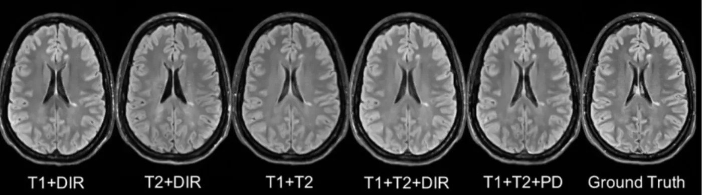
from different combinations of T1, T2, DIR and PD (see in Table 4(c) and Fig. 7). It indicates
that our method can be used to get an acceptable predicted FLAIR from the datasets which only
contain some sequences. From Table4(c)we can also infer that adding a pulse sequence improves
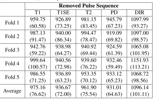
Table 4: FLAIR prediction results by using different input pulse sequences
(a) Mean Square Error (Standard Deviation)
Removed Pulse Sequence
T1 T1SE T2 PD DIR Fold 1 959.75 (60.58) 926.89 (73.25) 981.15 (83.45) 945.79 (67.23) 1097.99 (93.27) Fold 2 987.13 (91.47) 940.00 (86.34) 994.47 (78.47) 919.09 (69.82) 1097.00 (98.57) Fold 3 942.76 (59.22) 938.98 (64.27) 940.92 (69.44) 924.59 (61.39) 1065.08 (101.95) Fold 4 999.64 (100.57) 940.56 (72.98) 939.60 (76.22) 932.46 (59.49) 1151.93 (113.21) Fold 5 986.55 (71.25) 936.89 (63.23) 953.35 (70.12) 933.12 (65.23) 1068.72 (98.56) Average 975.16 (76.62) 936.67 (72.00) 961.90 (75.54) 931.01 (64.63) 1096.14 (101.11)
(b) Performance Comparison by removing DIR (Standard Deviation)
Random Forest 60 Multilayer
Perceptron U-Net Our Method Fold 1 1035.17 (102.37) 1589.62 (131.32) 1068.59 (100.28) 1097.99 (93.27) Fold 2 1167.52 (127.67) 1375.28 (121.12) 998.66 (106.79) 1097.00 (98.57) Fold 3 1170.36 (105.37) 1316.53 (128.46) 1135.24 (128.15) 1065.08 (101.95) Fold 4 1218.38 (129.01) 1235.26 (117.26) 1175.68 (107.33) 1151.93 (113.21) Fold 5 1189.64 (108.28) 1537.61 (135.78) 1003.54 (95.18) 1068.72 (98.56) Average 1156.21 (114.54) 1410.86 (126.79) 1076.34 (107.55) 1096.14 (101.11)
(c) Mean Square Error (Standard Deviation)
Input Pulse Sequences
T1+DIR T2+DIR T1+T2 T1+T2+DIR T1+T2+PD Fold 1 966.67 (70.12) 993.25 (99.35) 1375.83 (123.68) 926.88 (83.68) 1281.06 (112.57) Fold 2 953.87 (68.57) 974.88 (86.32) 1562.46 (132.68) 944.39 (79.23) 1324.17 (121.37) Fold 3 998.71 (84.90) 1007.69 (103.87) 1158.65 (112.29) 961.19 (71.68) 1261.68 (128.91) Fold 4 973.24 (77.79) 998.56 (98.23) 1078.67 (103.89) 931.47 (69.31) 1143.58 (98.95) Fold 5 968.55 (71.59) 986.57 (91.33) 1212.59 (126.79) 958.28 (73.45) 1156.79 (102.67) Average 972.21 (74.60) 992.19 (95.82) 1277.64 (119.87) 944.44 (75.47) 1233.46 (112.89)
Fig 7: Different Combinations of T1, T2, DIR and PD as input sequences.
Shown are synthesized FLAIR with different MRI pulse sequences as inputs from T1+DIR to T1+T2+PD. A better performance can be achieved when both DIR and T1 exist.
4 Discussion and Conclusion
We introduced 3D fully convolutional neural networks for FLAIR prediction from multiple MRI
pulse sequences, and a sequence-specific saliency map for investigating each pulse sequence
con-tribution. Even though the architecture of our method is simple, the nonlinear relationship between
the source images and FLAIR can be well captured by our network. Both the qualitative and
quanti-tative results have shown its competitive performance for FLAIR prediction. Compared to previous
methods, representative patches selection is not required so that this speeds up the training process.
Additionally, 2D Convolutional Neural Networks (2D CNNs) become popular in computer vision,
however they are not suitable to directly use 2D CNNs for volumetric medical image data. Unlike
Refs.19and9, our method can better keep the spatial information between slices. Moreover, the
generated FLAIR has a good contrast for MS lesions. In practice, in some datasets, not all the
subjects have all the pulse sequences. Our proposed P3S map can be used to reflect the impact
of each input pulse sequence on the prediction result so that the pulse sequences which contribute
very little can be removed. Furthermore, DIR is often used for the detection of MS cortical gray
FLAIR can be saved. Also, our P3S map can be generated by any kinds of neural networks trained
by standard backpropagation.
Our 3D FCNs have some limitations. The synthetic images appear slightly more blurred and
smoother than the ground truth. This maybe because we use a more traditional loss L2 distance as
our objective function. As mentioned in Ref.30, the use of L1 distance can encourage less blurring
and generate sharper image. Additionally, the proposed P3S is generated after the data
normaliza-tion which may affect the gradient. However, the network is changed as the normalizanormaliza-tion strategy
changes. And the saliency map is based on the network. Moreover, the dataset should be ideally
partitioned into training-validation-test sets. However, our dataset only has 24 subjects which is
quite small to split into training-validation-test set. Instead, we divided it into training-testing set
and the testing error is used as an estimate of the generalization error.
In the future, it would be interesting to also assess the utility of the method in the context
of other WM lesions (e.g. age-related WM hyperintensities). Specifically, FLAIR is the pulse
sequence of choice for studying different types of white matter lesions,31 including leucoaraiosis
(due to small vessel disease) that is commonly found in elderly subjects, that is associated to
cognitive decline and is a common co-pathology in neurodegenerative dementias.
Disclosures
Authors have no conflict of interest regarding this article.
Acknowledgments
The first author is funded by an Inria fellowship. The research leading to these results has received
Recherche-10-IA Institut Hospitalo-Universitaire-6) ANR-11-IDEX-004 (Agence Nationale de la
Recherche-11- Initiative d’Excellence-004, project LearnPETMR number SU-16-R-EMR-16), and
from the “Contrat d’Interface Local” program (to Dr Colliot) from Assistance Publique-Hˆopitaux
de Paris (AP-HP).
References
1 A. Compston and A. Coles, “Multiple sclerosis,” Lancet 372(9648), 1502–1517 (2008).
2 D. W. Paty, J. J. Oger, L. F. Kastrukoff, et al., “MRI in the diagnosis of MS: a prospective
study with comparison of clinical evaluation, evoked potentials, oligoclonal banding, and
CT,” Neurology 38, 180–185 (1988).
3 F. Barkhof, M. Filippi, D. H. Miller, et al., “Comparison of MRI criteria at first presentation
to predict conversion to clinically definite multiple sclerosis,” Brain 120 ( Pt 11), 2059–2069
(1997).
4 J. H. Woo, L. P. Henry, J. Krejza, et al., “Detection of simulated multiple sclerosis lesions on
t2-weighted and flair images of the brain: Observer performance,” Radiology 241(1), 206–
212 (2006).
5 S. G. Mueller, M. W. Weiner, L. J. Thal, et al., “The alzheimer’s disease neuroimaging
initia-tive,” Neuroimaging clinics of North America 15, 869–xii (2005).
6 J. E. Iglesias, E. Konukoglu, D. Zikic, et al., “Is synthesizing mri contrast useful for
inter-modality analysis?,” in Medical Image Computing and Computer-Assisted Intervention –
MICCAI 2013, LNCS 8149, Springer (2013).
clas-sification?,” in Medical Image Computing and Computer-Assisted Intervention – MICCAI
2015, LNCS 9349, Springer (2015).
8 S. Roy, A. Carass, N. Shiee, et al., “MR contrast synthesis for lesion segmentation,” in Proc
IEEE Int Symp Biomed Imaging, 932–935 (2010).
9 A. Jog, A. Carass, D. L. Pham, et al., “Random Forest FLAIR Reconstruction from T1, T2,
and PD -Weighted MRI,” Proc IEEE Int Symp Biomed Imaging 2014, 1079–1082 (2014).
10 T. Huynh, Y. Gao, J. Kang, et al., “Estimating CT Image From MRI Data Using Structured
Random Forest and Auto-Context Model,” IEEE Trans Med Imaging 35(1), 174–183 (2016).
11 N. Burgos, M. J. Cardoso, K. Thielemans, et al., “Attenuation correction synthesis for
hy-brid pet-mr scanners: Application to brain studies,” IEEE Transactions on Medical Imaging
33(12), 2332–2341 (2014).
12 K. He, X. Zhang, S. Ren, et al., “Deep residual learning for image recognition,” in 2016 IEEE
Conference on CVPR, 770–778, IEEE Computer Society (2016).
13 G. Chen, W. Choi, X. Yu, et al., “Learning efficient object detection models with
knowl-edge distillation,” in Advances in Neural Information Processing Systems 30, I. Guyon, U. V.
Luxburg, S. Bengio, et al., Eds., 742–751, Curran Associates, Inc. (2017).
14 E. Shelhamer, J. Long, and T. Darrell, “Fully convolutional networks for semantic
segmenta-tion,” IEEE Trans. Pattern Anal. Mach. Intell. 39(4), 640–651 (2017).
15 S. Zhou, H. Greenspan, and D. Shen, Deep Learning for Medical Image Analysis, Elsevier
Science (2017).
16 K. Bahrami, F. Shi, I. Rekik, et al., “Convolutional neural network for reconstruction of
and Data Labeling for Medical Applications, LABELS 2016, DLMIA 2016, LNCS 10008,
Springer (2016).
17 D. Nie, X. Cao, Y. Gao, et al., “Estimating ct image from mri data using 3d fully convolutional
networks,” in Deep Learning and Data Labeling for Medical Applications - LABELS 2016,
DLMIA 2016, LNCS 10008, 170–178, Springer (2016).
18 R. Li, W. Zhang, H.-I. Suk, et al., “Deep learning based imaging data completion for
im-proved brain disease diagnosis,” in Medical Image Computing and Computer-Assisted
Inter-vention – MICCAI 2014, LNCS 8675, 305–312, Springer International Publishing (2014).
19 V. Sevetlidis, M. V. Giuffrida, and S. A. Tsaftaris, “Whole image synthesis using a deep
encoder-decoder network,” in Simulation and Synthesis in Medical Imaging, SASHIMI 2016,
LNCS9968, 127–137, Springer (2016).
20 Y. LeCun, B. Boser, J. S. Denker, et al., “Backpropagation applied to handwritten zip code
recognition,” Neural Comput. 1, 541–551 (1989).
21 A. Krizhevsky, I. Sutskever, and G. E. Hinton, “Imagenet classification with deep
convolu-tional neural networks,” in NIPS 25, 1097–1105, Curran Associates (2012).
22 K. Simonyan, A. Vedaldi, and A. Zisserman, “Deep inside convolutional networks:
Visualis-ing image classification models and saliency maps,” CoRR abs/1312.6034 (2013).
23 N. J. Tustison, B. B. Avants, P. A. Cook, et al., “N4itk: Improved n3 bias correction,” IEEE
Transactions on Medical Imaging29, 1310–1320 (2010).
24 D. N. Greve and B. Fischl, “Accurate and robust brain image alignment using boundary-based
25 Theano Development Team, “Theano: A Python framework for fast computation of
mathe-matical expressions,” arXiv e-prints abs/1605.02688 (2016).
26 F. Chollet et al., “Keras.”https://github.com/fchollet/keras(2015).
27 D. H. Ye, D. Zikic, B. Glocker, et al., “Modality propagation: Coherent synthesis of
subject-specific scans with data-driven regularization,” in Medical Image Computing and
Computer-Assisted Intervention – MICCAI 2013, LNCS 8149, Springer (2013).
28 O. Ronneberger, P.Fischer, and T. Brox, “U-net: Convolutional networks for biomedical
im-age segmentation,” in Medical Imim-age Computing and Computer-Assisted Intervention
(MIC-CAI), LNCS 9351, 234–241, Springer (2015).
29 P. Coup´e, T. Tourdias, P. Linck, et al., “Lesionbrain: An online tool for white matter lesion
segmentation,” in International Workshop on Patch-based Techniques in Medical Imaging–
Patch-MI 2018, LNCS, Springer (2018).
30 P. Isola, J.-Y. Zhu, T. Zhou, et al., “Image-to-image translation with conditional adversarial
networks,” arxiv (2016).
31 J. Koikkalainen, H. Rhodius-Meester, A. Tolonen, et al., “Differential diagnosis of
neurode-generative diseases using structural mri data,” NeuroImage: Clinical 11, 435 – 449 (2016).
Wen Wei, MSc at University of Paris XI, is a PhD student in ARAMIS Laboratory and EPIONE
project team at Inria. His current research interests include deep learning for medical image
anal-ysis, medical image synthesis in particular for Multiple Sclerosis.
Emilie Poirion, MSc at UPMC paris VI, is a PhD student in the team Pr. Stankoff at the Brain and
applied to neurological disease, in particular Multiple Sclerosis.
Benedetta Bodini, MD-PhD, is an associate professor of neurology at Sorbonne-Universit´e in
Paris. She is part of the research team “Repair in Multiple Sclerosis, from basic science to clinical
translation”, at the Brain and Spinal Cord Institute (ICM) in Paris, where she studies the
mecha-nisms underlying the pathogenesis of multiple sclerosis using MRI and molecular imaging.
Stanley Durrleman, PhD, is the co-head of joint Inria/ICM Aramis Lab at the Brain and Spine
Institute (ICM) in Paris. He is also the coordinator of the ICM Center of Neuroinformatics, and
scientific director of the ICM platform of biostatistics and bioinformatics. His team focuses on the
development of new statistical and computational approaches for the analysis of image data and
image-derived geometric data such a surface meshes.
Olivier Colliot, PhD, is a Research Director at CNRS and the head of the ARAMIS Laboratory,
a joint laboratory between CNRS, Inria, Inserm and Sorbonne University within the Brain and
Spine Institute (ICM) in Paris, France. He received the PhD in Signal Processing from Telecom
ParisTech in 2003 and the Habilitation degree from University Paris-Sud in 2011. His research
interests include machine learning, medical image analysis and their applications to neurological
disorders.
Bruno Stankoff, MD-PhD, is a professor of neurology in Sorbonne-Universit´e in Paris. He leads
the Multiple Sclerosis (MS) center of Saint Antoine Hospital (AP-HP), and co-lead the research
team entitled “Repair in Multiple Sclerosis, from basic science to clinical translation”, at the Brain
network, OFSEP steering committee, ARSEP medico-scientific committee, French MS Society
(SFSEP).
Nicholas Ayache, PhD, is a member of the French Academy of Sciences and a Research
Direc-tor at Inria (French Research Institute for Computer Science and Applied Mathematics),
Sophia-Antipolis, France, where he leads the EPIONE project-team dedicated to e-Patients for e-Medicine.
His current research interests are in biomedical image analysis and simulation. He graduated from
Ecole des Mines de Saint-Etienne and holds a Ph.D. and a Th`ese d’Etat from University of
Paris-Sud (Orsay).
List of Figures
1 MRI pulse sequences usually used in a clinical setting.
T1-w provides an anatomical reference and T2-w is used for WM lesions visual-ization. However, on the T2-w, periventricular lesions are often indistinguishable from the adjacent cerebrospinal fluid (CSF) which is also of high signal. WM le-sions (red rectangles) characteristic of MS are best seen on FLAIR pulse sequence because of the suppression of the ventricular signal. Double inversion recovery (DIR) has direct application in MS for evaluating cortical pathology. Proton den-sity (PD) and T1 spin-echo (T1SE) are also used clinically.
2 The proposed 3D fully convolutional neural networks.
Our network architecture consists of three convolutional layers. The input layer is composed of 5 pulse sequences arranged as channels. The first layer extracts a 64-dimensional feature from input images through convolution process with a 3 × 3 × 3 × 5 × 64 kernel. The second and third layers apply the same convolution process to find a non-linear mapping for image prediction.
3 Comparison of Different Number of Layers.
Shown are learning curves for different number of layers (L = 2, 3, 4, 6). As the network goes deeper, the result can be increased. However, deeper structure cannot always lead to better results, sometimes even worse.
4 Qualitative comparison of the methods to predict FLAIR sequence.
Shown are synthetic FLAIR obtained by RF with 60 trees, MLP, U-Net, and our method followed by the true FLAIR. The 2nd and 4th rows show the absolute difference maps between each synthetic FLAIR and the ground truth.
5 Examples of WM lesion segmentation for a high and a low DICE.
The WM lesions are very small and diffuse, so even a slight difference in the over-lap can cause a big decrease for the DICE score. (a)(c) True FLAIR. (e)(g) Pre-dicted FLAIR. (b)(d) Segmentation of WM lesions (red) using true FLAIR. (f)(h) Segmentation of WM lesions using predicted FLAIR.
6 Pulse-Sequence-Specific Saliency Maps for input pulse Sequences.
The first row is the saliency maps for T1, T1SE, T2, PD, and DIR, respectively. And the second row is the corresponding multi-sequence MR images. It can be found that T1-w, DIR, and T2-w contribute more for FLAIR MRI prediction than PD or T1SE.
7 Different Combinations of T1, T2, DIR and PD as input sequences.
Shown are synthesized FLAIR with different MRI pulse sequences as inputs from T1+DIR to T1+T2+PD. A better performance can be achieved when both DIR and T1 exist.
List of Tables
1 Comparison of Different Number of Filters
2 Quantitative comparison between our method and other methods 3 Evaluation of MS lesion contrast (Standard Deviation)