HAL Id: hal-02549111
https://hal.archives-ouvertes.fr/hal-02549111v2
Preprint submitted on 30 Nov 2020
HAL is a multi-disciplinary open access
archive for the deposit and dissemination of
sci-entific research documents, whether they are
pub-lished or not. The documents may come from
teaching and research institutions in France or
abroad, or from public or private research centers.
L’archive ouverte pluridisciplinaire HAL, est
destinée au dépôt et à la diffusion de documents
scientifiques de niveau recherche, publiés ou non,
émanant des établissements d’enseignement et de
recherche français ou étrangers, des laboratoires
publics ou privés.
Gradient discretization of two-phase flows coupled with
mechanical deformation in fractured porous media
Francesco Bonaldi, Konstantin Brenner, Jérôme Droniou, Roland Masson
To cite this version:
Francesco Bonaldi, Konstantin Brenner, Jérôme Droniou, Roland Masson. Gradient discretization
of two-phase flows coupled with mechanical deformation in fractured porous media. 2020.
�hal-02549111v2�
Gradient discretization of two-phase flows coupled with mechanical
deformation in fractured porous media
Francesco Bonaldi∗1, Konstantin Brenner†1, Jérôme Droniou‡2, and Roland Masson§1
1Université Côte d’Azur, Inria, CNRS, Laboratoire J.A. Dieudonné, team Coffee, France 2School of Mathematics, Monash University, Victoria 3800, Australia
Abstract
We consider a two-phase Darcy flow in a fractured porous medium consisting in a matrix flow coupled with a tangential flow in the fractures, described as a network of planar surfaces. This flow model is also coupled with the mechanical deformation of the matrix assuming that the fractures are open and filled by the fluids, as well as small deformations and a linear elastic constitutive law. The model is discretized using the gradient discretization method [26], which covers a large class of conforming and non conforming schemes. This framework allows for a generic convergence analysis of the coupled model using a combination of discrete functional tools. Here, we describe the model together with its numerical discretization, and we prove a convergence result assuming the non-degeneracy of the phase mobilities and that the discrete solutions remain physical in the sense that, roughly speaking, the porosity does not vanish and the fractures remain open. This is, to our knowledge, the first convergence result for this type of models taking into account two-phase flows in fractured porous media and the non-linear poromechan-ical coupling. Previous related works consider a linear approximation obtained for a single phase flow by freezing the fracture conductivity [36,37]. Numerical tests employing the Two-Point Flux Approximation (TPFA) finite volume scheme for the flows and P2 finite elements for the mechanical deformation are also provided to illustrate
the behavior of the solution to the model. MSC2010: 65M12, 76S05, 74B10
Keywords: poromechanics, discrete fracture matrix models, two-phase Darcy flows, Gradient Discretization, con-vergence analysis
1
Introduction
Many real-life applications in geosciences involve processes like multi-phase flow and hydromechanical coupling in heterogeneous porous media. Such mathematical models are coupled systems of partial differential equations, including non-linear and degenerate parabolic ones. Besides the inherent difficulties posed by such equations, further complexities stem from the heterogeneity of the medium and the presence of discontinuities like fractures. This has a strong impact on the complexity of the models, challenging their mathematical and numerical analysis and the development of efficient simulation tools.
This work focuses on the so called hybrid-dimensional matrix fracture models obtained by averaging both the unknowns and the equations across the fracture width and by imposing appropriate transmission conditions at the matrix fracture interfaces. Given the high geometrical complexity of real-life fracture networks, the main advantages of these hybrid-dimensional compared with full-hybrid-dimensional models are to facilitate the mesh generation and the discretization of the model, and to reduce the computational cost of the resulting schemes. This type of hybrid-dimensional models has been the object of intensive researches over the last twenty years due to the ubiquity of fractures in geology and their large impact on flow, transport and mechanical behavior of rocks. For the derivation and analysis of such models, let us refer to [4,32,43,47,6,16,18,50] for single-phase Darcy flows, [11, 52, 49,39,17,27,19,2] for two-phase Darcy flows, and [44,45,41,36,37, 33, 42,34,56] for poroelastic models.
In this article, we consider the two-phase Darcy flow in a network of pre-existing fractures represented as pd ´ 1q-dimensional planar surfaces coupled with the surroundingd-dimensional matrix. The fractures are assumed to be open and filled by the fluids. Both phase pressures are assumed continuous across the fractures. This is a classical assumption for open fractures given the low pressure drop in the width of the fractures [11, 52,49, 17]. For single-phase flows, Poiseuille’s law is classically used to model the flow along the fractures. This leads to a Darcy-like tangential flow with
∗francesco.bonaldi@univ-cotedazur.fr †konstantin.brenner@univ-cotedazur.fr
‡Corresponding author,jerome.droniou@monash.edu §roland.masson@univ-cotedazur.fr
conductivity equal to d
3 f
12, wheredf is the fracture aperture [36,37]. Following [44], the extension to a two-phase flow is based on the generalized Darcy laws involving appropriate relative permeabilities and the capillary pressure-saturation relation. This hybrid-dimensional two-phase Darcy flow model is coupled with the matrix mechanical deformation assuming small strains and a linear poroelastic behavior [44,45,41]. The extension of the single-phase poromechanical coupling [36, 37,33, 42, 56] to two-phase Darcy flows is based on the so-called equivalent pressure used both in the matrix for the total stress and at both sides of the fractures as boundary condition for the mechanics. Typically, the equivalent pressure is defined as a convex combination of the phase pressures and several different combinations have been proposed in the literature [51]. Our choice of the equivalent pressure follows the pioneer monograph by Coussy [20] and involves the capillary energy which, as already noticed in [45, 41], plays a key role to obtain energy estimates for the coupled system. From the open fracture assumption, the fracture mechanical behavior reduces to the continuity of the normal stresses at both sides of the fracture matching with the fracture equivalent pressure times the unit normal vector. To our best knowledge, no theoretical or numerical analysis of the complete poromechanical model, with all non-linear coupling, has been carried out so far.
In this work, the hybrid-dimensional coupled model is discretized using the gradient discretization method (GDM) [26]. This framework is based on abstract vector spaces of discrete unknowns combined with reconstruction operators. The gradient scheme is then obtained by substitution of the continuous operators by their discrete counterparts in the weak formulation of the coupled model. The main asset of this framework is to enable a generic convergence analysis based on general properties of the discrete operators that hold for a large class of conforming and non conforming discretizations. Two essential ingredients to discretize the coupled model are the discretizations of the hybrid-dimensional two-phase Darcy flow and the discretization of the mechanics. Let us briefly mention, in both cases, a few families of discretizations typically satisfying the gradient discretization properties. For the discretization of the Darcy flow, the gradient discretization framework typically covers the case of cell-centered finite volume schemes with Two-Point Flux Approximation on strongly admissible meshes [43, 6, 2], or some symmetric Multi-Point Flux Approximations [55, 53, 3] on tetrahedral or hexahedral meshes. It also accounts for the families of Mixed Hybrid Mimetic and Mixed or Mixed Hybrid Finite Element discretizations such as in [4, 47,16, 18,7]. The case of vertex-based discretizations such as Control Volume Finite Element approaches (i.e. conforming finite element with mass lumping) [11, 52, 49] or the Vertex Approximate Gradient scheme [16, 18,17, 27, 19] is also accounted for. For the discretization of the elastic mechanical model, the gradient discretization framework covers conforming finite element methods such as in [36], as well as the Crouzeix-Raviart discretization [38,23], Discontinuous Galerkin methods [30], the Hybrid High Order discretization [22], and the Virtual Element Method [8]. Note that many of these methods are actually applicable to both the flow and the mechanical component of the model.
Without taking into account the poromechanical coupling, convergence results have been obtained in [6,4,47,16,18] for hybrid-dimensional single-phase Darcy flow models, and in [17,27] for hybrid-dimensional two-phase Darcy flow models. The well-posedness and convergence analysis of single-phase poromechanical models is studied in [36, 37]. Nevertheless those analyses consider a linear approximation of the coupled model obtained by freezing the fracture conductivity d
3 f
12, and hence eliminating the non-linear coupling between the fracture aperture and the Darcy flow. Let us also mention the related recent work [13] on unsaturated poroelasticity based on the Richards approximation of the two-phase flow model, using partial linearizations, non-degeneracy conditions and Kirchhoff transformation (which is made possible by assuming that the saturation–capillary pressure law is uniform across the domain). Note that fractures are not considered in this work.
Our main result is the proof of convergence, in the GDM setting, of the approximate solutions to the weak solution of the non-linear coupled model with two-phase flows. To our best knowledge, this is the first convergence result for this type of hybrid-dimensional model taking into account the full non-linear poromechanical coupling. The convergence result is established under the following main assumptions. It is first assumed that the approximate matrix porosity remains bounded below by a strictly positive constant and that the approximate fracture aperture remains larger than some given aperture vanishing only at the tips. Let us point out that these assumptions are due to the limitations of the model itself rather than to the shortcomings of the numerical analysis. They cannot be avoided since the continuous model does not ensure the positivity of the porosity nor of the fracture aperture, properties needed to guarantee existence of solutions. We note that previous works on similar models circumvent these limitations by linearization processes (complete or partial freezing of the matrix porosity and fracture apertures). Regarding the assumption on the fracture aperture, it could possibly be overcome by introducing contact mechanics in the model [33, 9]. This direction will be investigated in a future work. It is also assumed in the numerical analysis that the mobility functions are bounded below by strictly positive constants. Independently of the poromechanical coupling, this is a classical assumption to enable the stability and convergence analysis of two-phase Darcy flows with spatial discontinuity of the capillary pressure functions, as it is always the case in the presence of fractures (see [31,17, 27]). To our knowledge, the only convergence analyses covering both the degeneracy of the mobilities and discontinuous capillary pressures are limited to Two-Point Flux Approximations (see [14,15]). Extending such analyses, even considering only the TPFA method for the flow, to the poromechanical model considered here is far from straightforward and seems to bring additional challenges; given that our analysis is already quite technical, we postpone this extension to degenerate
mobility functions to a future work.
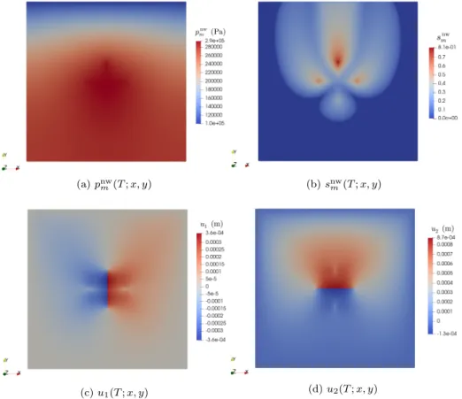
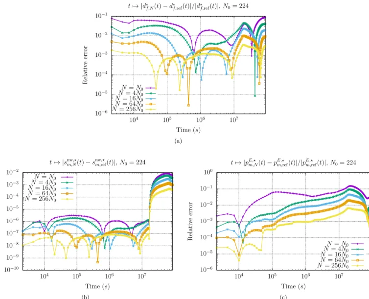
The rest of the article is organized as follows. Section2 introduces the continuous hybrid-dimensional coupled model. Section 3 describes the gradient discretization method for the coupled model including the definition of the recon-struction operators, the discrete variational formulation and the properties of the gradient discretization needed for the subsequent convergence analysis. Section 4 proceeds with the convergence analysis. The a priori estimates are established in Subsection 4.1, the compactness properties in Subsection 4.2and the convergence to a weak solution is proved in Subsection4.3. In Section 5, numerical experiments based on the Two-Point Flux Approximation finite volume scheme for the flows and second-order finite elements for the mechanical deformation are carried out for a cross-shaped fracture network in a two-dimensional porous medium, and illustrate the numerical convergence of the solution. AppendicesA.1andA.2state some technical results used in the convergence analysis.
2
Continuous model
We consider a bounded polytopal domain Ω of Rd, d P t2, 3u, partitioned into a fracture domain Γ and a matrix domainΩzΓ. The network of fractures is defined by
Γ “ď
iPI Γi
where each fractureΓi Ă Ω, i P I is a planar polygonal simply connected open domain with angles strictly lower than 2π. Without restriction of generality, we will assume that the fractures may intersect exclusively at their boundaries, that is for anyi, j P I, i ‰ j one has ΓiX Γj “ H, but not necessarily ΓiX Γj “ H. Since one can split a general (non-simply connected) planar polygon into several simply connected pieces intersecting only at their boundaries (see Figure 1) our assumptions on the fracture network are in fact quite general. Roughly speaking we only exclude the non-planar fractures.
Figure 1: Example of a 2D domainΩ with three intersecting fractures Γi,i P t1, 2, 3u.
The two sides of a given fracture ofΓ are denoted by ˘ in the matrix domain, with unit normal vectors n˘ oriented outward of the sides ˘. We denote by γ the trace operator on Γ for functions in H1pΩq, by γBΩthe trace operator for the same functions on BΩ, and byJ¨K the normal trace jump operator on Γ for functions in HdivpΩzΓq, defined by
J ¯uK “ ¯u
`¨ n`` ¯u´¨ n´ for all u P H¯
divpΩzΓq.
We denote by ∇τ the tangential gradient and by divτ the tangential divergence on the fracture network Γ. The symmetric gradient operator ε is defined such that εp¯vq “ 12p∇¯v `tp∇¯vqq for a given vector field ¯v P H1pΩzΓqd. The fracture aperture, denoted by ¯df, is defined by ¯df “ ´J ¯uK for a displacement field ¯u P H
1pΩzΓqd.
Let us fix a continuous functiond0: Γ Ñ p0, `8q vanishing at BΓzpBΓ X BΩq (i.e. at the tips of Γ) and taking strictly positive values at BΓ X BΩ. The discrete fracture aperture will be assumed to be greater than or equal to d0 almost everywhere (by the established convergence result, the same will hold for its limit). We note that the assumptions on d0are minimal, allowing for very general behavior of the fracture aperture at the tips.
Let us introduce some relevant function spaces:
U0“ t¯v P pH1pΩzΓqqd| γBΩv “ 0u¯ (1)
for the displacement vector, and
V0“ t¯v P H01pΩq | γ ¯v P Hd10pΓqu (2)
for each phase pressure, where the spaceH1
d0pΓq is made of functions vΓ inL
2
pΓq, such that d30{2∇τvΓ is inL2pΓqd´1, and whose traces are continuous at fracture intersections BΓiX BΓj, pi, jq P I ˆ I (i ‰ j) and vanish on the boundary BΓ X BΩ.
The matrix and fracture rock types are denoted by the indicesrt “ m and rt “ f , respectively, and the non-wetting and wetting phases by the superscriptsα “ nw and α “ w, respectively. Each rock type rt P tm, f u is characterized by its own set of mobility functions pηrtαqαPtnw,wu and capillary pressure-saturation relation pSrtαqαPtnw,wu.
Figure 2: Example of a 2D domainΩ with its fracture network Γ, the unit normal vectors n˘toΓ, the phase pressures ¯
pαin the matrix andγ ¯pαin the fracture network, the displacement vector fieldu, the matrix Darcy velocities q¯ α
mand
the fracture tangential Darcy velocities qαf integrated along the fracture width.
The PDEs model reads: find the phase pressuresp¯α,α P tnw, wu, and the displacement vector field ¯u, both satisfying homogeneous Dirichlet boundary conditions on BΩ, such that ¯pc“ ¯pnw´ ¯pwand, forα P tnw, wu,
$ ’ ’ ’ ’ ’ ’ ’ ’ ’ ’ ’ & ’ ’ ’ ’ ’ ’ ’ ’ ’ ’ ’ % Bt `¯ φmSmαp ¯pcq ˘ ` div pqαmq “ hαm on p0, T q ˆ ΩzΓ, qαm“ ´ηmαpSmαp ¯pcqqKm∇¯pα on p0, T q ˆ ΩzΓ, Bt´ ¯dfSαfpγ ¯pcq ¯ ` divτpqαfq ´Jq α mK “ h α f on p0, T q ˆ Γ, qαf “ ´ηfαpSfαpγ ¯pcqqp 1 12d¯ 3 fq∇τγ ¯pα on p0, T q ˆ Γ, ´div ´ σp¯uq ´ b ¯pE mI ¯ “ f on p0, T q ˆ ΩzΓ σp¯uq “ 2µ εp¯uq ` λ divp¯uq I on p0, T q ˆ ΩzΓ, (3) with $ ’ ’ & ’ ’ % Btφ¯m“ b divBtu `¯ 1 MBtp¯ E m on p0, T q ˆ ΩzΓ, pσp¯uq ´ b ¯pE mIqn˘“ ´ ¯pEfn˘ on p0, T q ˆ Γ, ¯ df “ ´J ¯uK on p0, T q ˆ Γ, (4)
and the initial conditions
¯ pα
|t“0“ ¯pα0, φ¯m|t“0“ ¯φ0m.
Here, we have denoted byp¯c the capillary pressure, and the equivalent pressuresp¯mE andp¯Ef are defined, following [20], by ¯ pEm“ ÿ αPtnw,wu ¯ pαSαmp ¯pcq ´ Ump ¯pcq, p¯Ef “ ÿ αPtnw,wu γ ¯pαSfαpγ ¯pcq ´ Ufpγ ¯pcq, where Urtp ¯pcq “ żp¯c 0 z pSnwrt q 1 pzq dz (5)
is the capillary energy density function of the rock typert P tm, f u. As already noticed in [45,41], this is a key choice to obtain the energy estimates that are the starting point for the convergence analysis.
We make the following main assumptions on the data:
(H1) For each phaseα P tnw, wu and rock type rt P tm, f u, the mobility function ηα
rt is continuous, non-decreasing, and there exist0 ă ηα
rt,minď ηαrt,maxă `8 such that ηαrt,minď ηrtαpsq ď ηrt,maxα for alls P r0, 1s. (H2) For each rock type rt P tm, f u, the non-wetting phase saturation function Snw
rt is a non-decreasing Lipschitz continuous function with values in r0, 1s, and Srtw“ 1 ´ Srtnw.
(H3) b P r0, 1s is the Biot coefficient, M ą 0 is the Biot modulus, and λ ą 0, µ ą 0 are the Lamé coefficients. These coefficients are assumed to be constant for simplicity.
(H4) The initial pressures are such thatp¯α
0 P V0X L8pΩq and γ ¯pα0 P L8pΓq, α P tnw, wu; the initial porosity is such that ¯φ0
(H5) The source terms satisfy f P L2pΩqd,hα
mP L2pp0, T q ˆ Ωq, and hαf P L2pp0, T q ˆ Γq. (H6) The matrix permeability tensor Km is symmetric and uniformly elliptic onΩ.
Definition 2.1 (Weak solution of the model). A weak solution of the model is given byp¯αP L2p0, T ; V
0q, α P tnw, wu, andu P L¯ 8p0, T ; U
0q, such that, for any α P tnw, wu, ¯d
3{2
f ∇τγ ¯pαP L2pp0, T q ˆ Γqqd´1and, for allϕ¯αP Cc8pr0, T q ˆ Ωq and all smooth functionsv¯ : r0, T s ˆ pΩzΓq Ñ Rd vanishing on BΩ and whose derivatives of any order admit finite limits on each side ofΓ,
żT 0 ż Ω ´ ´ ¯φmSmαp ¯pcqBtϕ¯α` ηmαpSαmp ¯pcqqKm∇¯pα¨∇ ¯ϕα ¯ dxdt ` żT 0 ż Γ ´ ´ ¯dfSfαpγ ¯pcqBtγ ¯ϕα` ηαfpSfαpγ ¯pcqq ¯ d3 f 12∇τγ ¯p α ¨∇τγ ¯ϕα ¯ dσpxqdt ´ ż Ω ¯ φ0 mSmαp ¯p0cq ¯ϕαp0, ¨qdx ´ ż Γ ¯ d0 fSfαpγ ¯p0cqγ ¯ϕαp0, ¨qdσpxq “ żT 0 ż Ω hα mϕ¯αdxdt ` żT 0 ż Γ hα fγ ¯ϕαdσpxqdt, (6) żT 0 ż Ω ´ σp¯uq : εp¯vq ´ b ¯pEmdivp¯vq ¯ dxdt ` żT 0 ż Γ ¯ pEf J¯vK dσpxqdt “ żT 0 ż Ω f ¨ ¯v dxdt, (7) withp¯c“ ¯pnw´ ¯pw, ¯df “ ´J ¯uK,φ¯m´ ¯φ 0 m“ b divp¯u ´ ¯u0q ` 1 Mp ¯p E m´ ¯pE,0m q, ¯d0f “ ´J ¯u 0 K, where ¯u 0is the solution of (7) without the time integral and using the initial equivalent pressuresp¯E,0
m and p¯
E,0
f obtained from the initial pressures ¯
pα
0 andγ ¯pα0, α P tnw, wu.
Remark 2.2 (Regularity of the fracture aperture). Notice that, by the Sobolev–trace embeddings [1, Theorem 4.12], ¯
u P L8p0, T ; U
0q implies that ¯df “ ´J ¯uK P L
8p0, T ; L4pΓqq. All the integrals above are thus well-defined.
3
The gradient discretization method
The gradient discretization (GD) for the Darcy continuous pressure model, introduced in [16], is defined by a finite-dimensional vector space of discrete unknownsX0
Dp and
• two discrete gradient linear operators on the matrix and fracture domains ∇m Dp: X 0 DpÑ L 8 pΩqd, ∇fDp: X 0 Dp Ñ L 8 pΓqd´1; • two function reconstruction linear operators on the matrix and fracture domains
Πm Dp : X 0 DpÑ L 8 pΩq, ΠfDp: XD0pÑ L8pΓq, which are piecewise constant [26, Definition 2.12].
A consequence of the piecewise-constant property is the following: there is a basis peiqiPI of XD0p such that, if
v “ ř
iPIviei and if, for a mapping g : R Ñ R with gp0q “ 0, we define gpvq “ řiPIgpviqei P XD0p by applyingg component-wise, thenΠrt
Dpgpvq “ gpΠ
rt
Dpvq for rt P tm, f u. Note that the basis peiqiPI is usually canonical and chosen
in the design ofX0
Dp. The vector space X
0 Dp is endowed with }v}Dp– }∇ m Dpv}L2pΩq` }d 3{2 0 ∇ f Dpv}L2pΓq,
assumed to define a norm onX0 Dp.
The gradient discretization for the mechanics is defined by a finite-dimensional vector space of discrete unknownsX0 Du
and
• a symmetric gradient linear operator εDu : X
0
Du Ñ L
2pΩ,S dpRqq, • a displacement function reconstruction linear operator ΠDu : X
0
Du Ñ L
• a normal jump function reconstruction linear operatorJ¨KDu : X
0
Du Ñ L
4 pΓq,
where SdpRq is the vector space of real symmetric matrices of size d. Let us define the divergence and stress tensor operators by
divDupvq “ TracepεDupvqq and σDupvq “ 2µεDupvq ` λ divDupvqI,
and the fracture widthdf,Du “ ´JuKDu. It is assumed that the following quantity defines a norm onX
0 Du:
}v}Du – }εDupvq}L2pΩ,SdpRqq.
A spatial GD can be extended into a space-time GD by complementing it with • a discretization 0 “ t0ă t1ă ¨ ¨ ¨ ă tN “ T of the time interval r0, T s; • interpolators IDp: V0Ñ X 0 Dp andI m Dp: L 2 pΩq Ñ XD0p of initial conditions. Forn P t0, . . . , N u, we denote by δtn`1
2 “ tn`1´ tn the time steps, and by ∆t “ maxn“0,...,Nδtn`12 the maximum
time step.
The spatial operators are extended into space-time operators as follows. Let χ represent either p or u. If w “ pwnqNn“0P pXD0χq
N `1, and Ψ
Dχ is a spatial GD operator, its space-time extension is defined by
ΨDχwp0, ¨q “ ΨDχw0and, @n P t0, . . . , N ´ 1u , @t P ptn, tn`1s, ΨDχwpt, ¨q “ ΨDχwn`1.
For convenience, the same notation is kept for the spatial and space-time operators. Moreover, we define the discrete time derivative as follows: forf : r0, T s Ñ L1
pΩq piecewise constant on the time discretization, with fn “ f|ptn´1,tns
andf0“ f p0q, we set δtf ptq “ fn`1´fn
δtn` 12 for allt P ptn, tn`1s, n P t0, . . . , N ´ 1u.
Notice that the space of piecewise constantX0
Dχ-valued functionsf on the time discretization together with the initial
valuef0“ f p0q can be identified with pXD0χqN `1. The same definition of discrete derivative can thus be given for an element w P pX0
Dχq
N `1. Namely, δ
tw P pXD0χqN is defined by setting, for anyn P t0, . . . , N ´ 1u and t P ptn, tn`1s, δtwptq “ pδtwqn`1 – wn`1´wn
δtn` 12
. If ΨDχpt, ¨q is a space-time GD operator, by linearity the following commutativity
property holds: ΨDχδtwpt, ¨q “ δtpΨDχwpt, ¨qq.
The gradient scheme for the system consists in replacing the “continuous” functional space and differential operators in (6)–(7) by their discrete counterparts. This results in the following discrete problem: findpαP pX0
Dpq
N `1,α P tnw, wu, and u P pXD0uqN `1, such that for allϕαP pX0
Dpq N `1, v P pX0 Duq N `1andα P tnw, wu, żT 0 ż Ω ´ δt ´ φDΠmDps α m ¯ ΠmDpϕα` ηmαpΠmDps α mqKm∇mDpp α ¨∇mDpϕα ¯ dxdt ` żT 0 ż Γ δt ´ df,DuΠ f Dps α f ¯ ΠfDpϕαdσpxqdt ` żT 0 ż Γ ηαfpΠ f Dps α fq d3 f,Du 12 ∇ f Dpp α ¨∇fDpϕαdσpxqdt “ żT 0 ż Ω hαmΠmDpϕ αdxdt `żT 0 ż Γ hαfΠ f Dpϕ αdσpxqdt, (8a) żT 0 ż Ω ´ σDupuq : εDupvq ´ b Π m Dpp E m divDupvq ¯ dxdt ` żT 0 ż Γ ΠfDppEf JvKDudσpxqdt “ żT 0 ż Ω f ¨ ΠDuv dxdt, (8b)
with the closure equations $ ’ ’ ’ ’ ’ ’ ’ ’ ’ ’ ’ & ’ ’ ’ ’ ’ ’ ’ ’ ’ ’ ’ % pc“ pnw´ pw, sαm“ Smαppcq, sαf “ Sfαppcq, pE m“ ÿ αPtnw,wu pαsα m´ Umppcq, pEf “ ÿ αPtnw,wu pαsα f ´ Ufppcq, φD´ ΠmDpφ0m“ b divDupu ´ u 0 q `M1ΠmDpppEm´ pE,0m q, df,Du “ ´JuKDu, σDupvq “ 2µεDupvq ` λ divDupvqI. (8c)
The initial conditions are given by pα 0 “ IDpp¯ α 0 (α P tnw, wu), φ0m “ IDmp ¯ φ0
m, and the initial displacement u0 is the solution of (8b) without the time variable and with the equivalent pressures obtained from the initial pressures ppα0qαPtnw,wu.
Remark 3.1 (Non-homogeneous boundary conditions). The homogeneous Dirichlet boundary conditions are embedded in the discrete spacesXD0p and XD0u. Non-homogeneous (or other types of) boundary conditions are equally easy to handle in the GDM setting [26, Section 2.2 and Chapter 3].
Remark 3.2 (GDM framework). As shown above, the GDM framework enables a presentation of the schemes in a way that is almost as compact as the weak formulation itself (compare with Definition2.1). This presentation is valid for conforming methods, that already have a compact writing but may not be the best suited in practical applications (especially for the flow component), but also for non-conforming methods of practical interest in engineering; explicitly writing, for example, the TPFA formulation for the flow component of the model would lead to much lengthier equations. Additionally, the GDM analysis is also carried out in a compact way, identifying key properties and manipulating discrete equations almost as their continuous counterparts; notwithstanding the fact that this analysis applies to many different methods at once, developing it for a given specific scheme would not lead to any simplification – the complexity in the upcoming analysis comes from the poromechanical model we consider, not from the numerical analysis framework we use.
3.1
Properties of gradient discretizations
Let pDlpqlPN and pDluqlPN be sequences of GDs. We state here the assumptions on these sequences which ensure that the solutions to the corresponding schemes converge. Most of these assumptions are adaptation of classical GD assumptions [26], except for the chain-rule, product rule and cut-off properties used in Subsection4.2 to obtain compactness properties; we note that all these assumptions hold for standard discretizations used in porous media flows.
Following [16], the spatial GD of the Darcy flowDp“ ´ X0 Dp,∇ m Dp,∇ f Dp, Π m Dp, Π f Dp ¯
is assumed to satisfy the following coercivity, consistency, limit-conformity and compactness properties.
Coercivity ofDp. LetCDpą 0 be defined by
CDp“ max 0‰vPX0 Dp }ΠmDpv}L2pΩq` }ΠfD pv}L2pΓq }v}Dp . (9)
Then, a sequence of spatial GDs pDl
pqlPNis said to be coercive if there existsCpą 0 such that CDl
pď Cpfor alll P N.
Consistency of Dp. Letr ą 8 be given, and for all w P V0 andv P XD0p let us define SDppw, vq “ }∇ m Dpv ´∇w}L2pΩq` }∇ f Dpv ´∇τγw}LrpΓq ` }ΠmDpv ´ w}L2pΩq` }Πf Dpv ´ γw}LrpΓq, (10) andSDppwq “ minvPX0
DpSDppw, vq. Then, a sequence of spatial GDs pD
l
pqlPNis said to be consistent if for all w P V0 one haslimlÑ`8SDl
ppwq “ 0. Moreover, if pD
l
pqlPN is a sequence of space-time GDs, then it is said to be consistent if the underlying sequence of spatial GDs is consistent as above, and if, for anyϕ P V0 andψ P L2pΩq, as l Ñ `8,
∆tlÑ 0 , }ΠmDl pIDlpϕ ´ ϕ}L2pΩq` }Π f Dl pID l pϕ ´ ϕ}L2pΓqÑ 0 and }Π m Dl pI m Dl pψ ´ ψ}L2pΩqÑ 0. (11)
Remark 3.3 (Consistency). In [16], the consistency is only considered forr “ 2. As it will appear clear in the analysis, dealing with the coupling and non-linearity of the model requires us to adopt here a slightly stronger consistency assumption. Under standard mesh regularity assumptions, this stronger consistency property is still satisfied for all classical GDs [26, Part III].
Limit-conformity of Dp. For all prm, rfq P C8pΩzΓqdˆ C8pΓqd´1 andv P XD0p, let us define
WDpprm, rf, vq “ ż Ω ´ rm¨∇mDpv ` ΠmDpv divprmq ¯ dx ` ż Γ ´ rf¨∇fDpv ` ΠDfpv pdivτprfq ´JrmKq ¯ dσpxq, (12)
andWDpprm, rfq “ max
0‰vPX0
Dp
|WDpprm, rf, vq|
}v}Dp
. Then, a sequence of spatial GDs pDlpqlPN is said to be limit-conforming if for all prm, rfq P C8pΩzΓqdˆ Cc8pΓqd´1 one haslimlÑ`8WDl
pprm, rfq “ 0. Here C
8
c pΓqd´1 denotes the space of functions whose restriction to eachΓi is in C8pΓiqd´1 tangent to Γi, compactly supported away from the tips, and satisfying normal flux conservation at fracture intersections not located at the boundary BΩ.
Remark 3.4 (Compactly supported fluxes). The role of prm, rfq is that of test functions (they do not represent the continuous fluxes), to show that the limits of the discrete fluxes are indeed the continuous fluxes, see [16, Lemma 5.5]. (Local) compactness of Dp. A sequence of spatial GDs pDplqlPN is said to be locally compact if for all sequences pvlqlPNP pXD0l
pqlPNsuch that suplPN}v
l }Dl
p ă `8 and all compact sets KmĂ Ω and Kf Ă Γ, such that Kf is disjoint
from the intersections pΓiX Γjqi“j, the sequences pΠmDl pv
lq
lPN and pΠfDl pv
lq
lPN are relatively compact inL2pKmq and L2
pKfq, respectively.
Remark 3.5 (Local compactness through estimates of space translates). ForKm, Kf as above, set
TDl p,Km,Kfpξ, ηq “ max vPX0 Dlpzt0u }ΠmDl pvp¨ ` ξq ´ Π m Dl pv}L 2pK mq` ř iPI}Π f Dl pvp¨ ` ηiq ´ Π f Dl pv}L 2pK fXΓiq }v}Dl p , where ξ P Rd, η “ pη
iqiPI withηi tangent to Γi; for ξ and η small enough, this expression is well defined since Km and Kf are compact in Ω and Γ, respectively. Following [26, Lemma 2.21], An equivalent formulation of the local compactness property is: for allKm, Kf as above,
lim
ξ,ηÑ0suplPNTDlp,Km,Kfpξ, ηq “ 0.
Remark 3.6 (Usual compactness property for GDs). The standard compactness property for GD is not local but global, that is, on the entire domain and not any of its compact subsets (see, e.g., [26, Definition 2.8] and also below forDu). Two reasons pushed us to consider here the weaker notion of local compactness: firstly, for standard GDs, the global compactness does not seem obvious to establish (or even true) in the fractures, because of the weightd0 in the norm } ¨ }Dp, which prevents us from estimating the translates of the reconstructed function by the gradient near the fracture
tips; secondly, we will only prove compactness on saturations, which are uniformly bounded by 1 and for which local and global compactness are therefore equivalent.
In the following, for brevity we refer to the local compactness of pDlpqlPNsimply as the compactness of this sequence of GDs.
Chain rule estimate on pDlpqlPN: for any Lipschitz-continuous functionF : R Ñ R, there is CF ě 0 such that, for alll P N, v P X0 Dl p, }∇mDl pF pvq}L 2pΩqď CF}∇m Dl pv}L 2pΩq.
Product rule estimate on pDl
pqlPN: there existsCP such that, for anyl P N and any ul, vlP XD0l
p, it holds }∇mDppulvlq}L2pΩqď CP ´ |ul|8}∇mDpvl}L2pΩq` |vl|8}∇mD pu l }L2pΩq ¯ , where |w|8 – maxiPI|wi| whenever w “řiPIwiei with peiqiPI the canonical basis ofXD0l
p.
Cut-off property of pDl
pqlPN: for any compact setK Ă ΩzΓ, there exists CK ě 0 and pψlqlPNP pXD0l
pqlPN such that
p|ψl|8qlPNis bounded and, forl large enough: ΠmDl pψ l ě 0 on Ω; ΠmDl pψ l “ 1 on K; }∇mDl pψ l }L2pΩqď CK ΠfDl ppv lψl q “ 0 and ∇fDl ppv lψl q “ 0 for allvlP XD0l p
Coercivity of pDulqlPN. LetCDu ą 0 be defined by
CDu “ max 0‰vPX0 Dlu }ΠDl uv}L2pΩq` }JvKDul}L4pΓq }v}Dl u . (13)
Then, the sequence of spatial GDs pDluqlPN is said to be coercive if there existsCuą 0 such that CDl
u ď Cu for all
Consistency of pDulqlPN. For all w P U0, it holds limlÑ`8SDl upwq “ 0 where SDl upwq “ min vPX0 Dlu ” }εDl upvq ´ εpwq}L2pΩ,SdpRqq` }ΠDluv ´ w}L2pΩq` › ›JvKDl u´JwK › › L4pΓq ı . (14) Limit-conformity of pDl
uqlPN. Let CΓ8pΩzΓ,SdpRqq denote the vector space of smooth functions τ : ΩzΓ ÑSdpRq whose derivatives of any order admit finite limits on each side of Γ, and such that τ`pxqn` ` τ´pxqn´ “ 0 and pτ`pxqn`qˆn`“ 0 for a.e. x P Γ. For all τ P CΓ8pΩzΓ,SdpRqq, it holds limlÑ`8WDl
upτq “ 0 where WDl upτq “ max 0‰vPX0 Dlu 1 }v}Dl u „ż Ω ´ τ: εDl upvq ` ΠDluv ¨ divpτq ¯ dx ´ ż Γ pτn`q ¨ n`JvKDuldσpxq .
Compactness of pDluqlPN. For any sequence pvlqlPNP pXD0l
uqlPN such that suplPN}v
l }Dl u ă `8, the sequences pΠDl uv l qlPNand pJv l
KDluqlPNare relatively compact inL 2
pΩqd and inLs
pΓq for all s ă 4, respectively.
Remark 3.7 (Compactness through estimates of space translates). Similarly to Remark3.5(see also [26, Lemma 2.21]), the compactness of pDulqlPN is equivalent to
lim ξ,ηÑ0suplPNTDlu,spξ, ηq “ 0 @s ă 4, where TDl u,spξ, ηq “ max vPX0 Dluzt0u }ΠDl uvp¨ ` ξq ´ ΠDluv}L2pΩq` ř iPI › ›JvlKDl up¨ ` ηiq ´Jv l KDul › › LspΓ iq }v}Dl u , withξ P Rd,η “ pη
iqiPI withηi tangent toΓi, and the functions extended by 0 outside their respective domain Ω or Γ.
4
Convergence analysis
The main result of this work is the following theorem stating the convergence of the sequence of discrete solutions to a weak solution up to a subsequence.
Theorem 4.1 (Convergence to a weak solution). Let pDplqlPN, pDluqlPN, tptlnqN
l
n“0ulPN (where Nl is the number of time steps ofDpl), be sequences of space time GDs assumed to satisfy the coercivity, consistency, limit-conformity and compactness properties. Letφm,miną 0 and assume that, for each l P N, the gradient scheme (8a)–(8b) has a solution pα l P pXD0l pq Nl `1,α P tnw, wu, ul P pXD0l uq Nl `1 such that (i) df,Dl upt, xq ě d0pxq for a.e. pt, xq P p0, T q ˆ Γ,
(ii) φDlpt, xq ě φm,min for a.e. pt, xq P p0, T q ˆ Ω.
Then, there exist p¯α
P L2p0, T ; V0q, α P tnw, wu, and ¯u P L8p0, T ; U0q satisfying the weak formulation (6)–(7) such that forα P tnw, wu and up to a subsequence
Πm Dl pp α l á ¯pα weakly inL2p0, T ; L2pΩqq, ΠfDl pp α l á γ ¯pα weakly inL2p0, T ; L2pΓqq, ΠDl uu l á ¯u weakly-‹ in L8p0, T ; L2 pΩqdq, φDlá ¯φm weakly-‹ in L8p0, T ; L2pΩqq, df,Dl uÑ ¯df inL 8p0, T ; LppΓqq for 2 ď p ă 4, Πm Dl pS α mpplcq Ñ Smαp ¯pcq inL2p0, T ; L2pΩqq, ΠfDl pS α fpplcq Ñ Sfαpγ ¯pcq inL2p0, T ; L2pΓqq, where ¯φm“ ¯φ0m` b divp¯u ´ ¯u0q ` 1 Mp ¯p E m´ ¯pE,0m q, ¯df “ ´J ¯uK, and ¯pc“ ¯p nw ´ ¯pw.
Remark 4.2 (Discrete porosity and fracture aperture). As mentioned in the introduction, the assumptions that the discrete porosity and fracture aperture remain bounded below is a requirement coming from the model itself (which does not account for possible contact). It is not a fundamental restriction of the numerical framework and analysis.
We first present in Subsections 4.1 and 4.2 a sequence of intermediate results that will be useful for the proof of Theorem4.1detailed in Subsection4.3.
Remark 4.3 (Incompressible limit for the solid matrix). The above convergence result also holds when1{M “ 0, i.e., in the incompressible limit for the grains of the solid matrix (M Ñ `8). Indeed, in this case, Lemma4.4below does not ensureL8pL2q-boundedness of the reconstructed matrix equivalent pressure. Nevertheless, L2pL2q-boundedness for this quantity (needed in the proof of the above theorem, cf. Subsection4.3) can be readily inferred, based on the L2pL2q-boundedness of the reconstructed phase pressures (resulting from Lemma 4.4), the fact that reconstructed saturations are bounded, and the definition (5) of the capillary energy density.
4.1
Energy estimates
Using the phase pressures and velocity (time derivative of the displacement field) as test functions, the following a priori estimates can be inferred.
Lemma 4.4 (A priori estimates). Letpα, u be a solution to problem (8) such that (i) df,Dupt, xq ě d0pxq for a.e. pt, xq P p0, T q ˆ Γ,
(ii) φDpt, xq ě φm,min for a.e. pt, xq P p0, T q ˆ Ω, where φm,miną 0 is a constant.
Under hypotheses (H1)–(H6), there exists a real numberC ą 0 depending on the data, the coercivity constants CDp,
CDu, andφm,min, such that the following estimates hold:
}∇mDppα}L2pp0,T qˆΩqď C, }d 3{2 f,Du∇ f Dpp α }L2pp0,T qˆΓqď C, }UmpΠmDppcq}L8p0,T ;L1pΩqqď C, }d0UfpΠfDppcq}L8p0,T ;L1pΓqqď C, }ΠmDppEm}L8p0,T ;L2pΩqqď C, }εDupuq}L8p0,T ;L2pΩ,S dpRqqqď C, }df,Du}L8p0,T ;L4pΓqq ď C. (15)
Proof. For a piecewise constant functionv on r0, T s with vptq “ vn`1for all t P ptn, tn`1s, n P t0, . . . , N ´ 1u, and the initial valuevp0q “ v0, we define the piecewise constant functionv such that ˆˆ vptq “ vn for allt P ptn, tn`1s. We notice the following expression for the discrete derivative of the product of two such functions:
δtpuvqptq “ ˆuptqδtvptq ` vptqδtuptq. (16)
In (8a), upon choosing ϕα“ pα we obtainT
1` T2` T3` T4“ T5` T6, with T1“ żT 0 ż Ω δt ´ φDΠmDps α m ¯ ΠmDppαdxdt, T2“ żT 0 ż Ω ηαmpΠmDps α mqKm∇mDpp α ¨∇mDppαdxdt, T3“ żT 0 ż Γ δt ´ df,DuΠ f Dps α f ¯ ΠfDppαdσpxqdt, T4“ żT 0 ż Γ ηfαpΠ f Dps α fq d3 f,Du 12 ∇ f Dpp α ¨∇fD pp αdσpxqdt, T5“ żT 0 ż Ω hαmΠmDpp αdxdt, T 6“ żT 0 ż Γ hαfΠ f Dpp αdσpxqdt. (17)
First, we focus on the matrix and fracture accumulation termsT1 andT3, respectively. Using (16) and the piecewise constant function reconstruction property ofΠrt
Dp,rt P tm, f u, we can write δtpφDSmαpΠDmppcqq “ ˆφDδtS α mpΠmDppcq ` S α mpΠmDppcqδtφD, δtpdf,DuS α fpΠ f Dppcqq “ ˆdf,DuδtS α fpΠ f Dppcq ` S α fpΠ f Dppcqδtdf,Du.
Summing onα P tw, nwu, we obtain ÿ α pT1` T3q “ ÿ α ´żT 0 ż Ω ˆ φDΠmDpp αδ tSmαpΠmDppcqdxdt ` żT 0 ż Ω SmαpΠmDppcqΠ m Dpp αδ tφDdxdt ` żT 0 ż Γ ˆ df,DuΠ f Dpp αδ tSfαpΠ f Dppcqdσpxqdt ` żT 0 ż Γ SfαpΠ f DppcqΠ f Dpp αδ tdf,Dudσpxqdt ¯ . Now, forrt P tm, f u, ÿ α ΠDrtppαδtSrtαpΠrtDppcq “ Π rt DppcδtS nw rt pΠrtDppcq ě δtUrtpΠ rt Dppcq. (18)
Indeed, forn P t0, . . . , N ´ 1u, by the definition (5) of the capillary energyUrt and lettingπrtc,n“ ΠrtDppc,n, we have πc,n`1rt pSrtnwpπrtc,n`1q ´ Srtnwpπc,nrt qq “ Urtpπc,n`1rt q ´ Urtpπc,nrt q ` żπrt c,n`1 πrt c,n pSrtnwpqq ´ Srtnwpπc,nrt qqdq ě Urtpπc,n`1rt q ´ Urtpπc,nrt q,
where the last inequality holds sinceSrtnw is a non-decreasing function. Thus, we obtain ÿ α pT1` T3q ě żT 0 ż Ω ˆ φDδtUmpΠmDppcqdxdt ` żT 0 ż Γ ˆ df,DuδtUfpΠ f Dppcqdσpxqdt `ÿ α ´żT 0 ż Ω SmαpΠmDppcqΠ m Dpp αδ tφDdxdt ` żT 0 ż Γ SfαpΠ f DppcqΠ f Dpp αδ tdf,Dudσpxqdt ¯ . Applying again (16), we have
ˆ φDδtUmpΠmDppcq “ δtpφDUmpΠ m Dppcqq ´ UmpΠ m DppcqδtφD, ˆ df,DuδtUfpΠ f Dppcq “ δtpdf,DuUfpΠ f Dppcqq ´ UfpΠ f Dppcqδtdf,Du.
In the light of the closure equations (8c), this allows us to infer that ÿ α pT1` T3q ě żT 0 ż Ω δtpφDUmpΠmDppcqqdxdt ` żT 0 ż Γ δtpdf,DuUfpΠ f Dppcqqdσpxqdt ` żT 0 ż Ω 1 2Mδt ´ ΠmDppEm ¯2 dxdt ` żT 0 ż Ω b ΠmDppEmdivDupδtuqdxdt ´ żT 0 ż Γ ΠfDppEf JδtuKDudσpxqdt, (19)
where we have used the fact that
vδtv ě δt ˆ v2
2 ˙
(20) forv piecewise constant on r0, T s. Then, taking into account assumptions(H1)–(H6)and (i) in the lemma, there exists a real numberC ą 0 depending only on the data such that
ÿ α pT2` T4q ě C ´żT 0 ż Ω ÿ α |∇mDppα|2dxdt ` żT 0 ż Γ ÿ α |d3f,{2D u∇ f Dpp α |2dσpxqdt¯. (21)
On the other hand, upon choosing v “ δtu in (8b), we getT7` T8` T9“ T10, with T7“ żT 0 ż Ω σDupuq : εDupδtuqdxdt, T8“ ´ żT 0 ż Ω b ΠmDppEmdivDupδtuqdxdt T9“ żT 0 ż Γ ΠfDppEf JδtuKDudσpxqdt, T10“ żT 0 ż Ω f ¨ ΠDupδtuqdxdt. (22)
Using (20) and developping the definition of σDupuq, we see that T7ě żT 0 ż Ω δt ´1 2σDupuq : εDupuq ¯ dxdt, (23)
so that, all in all, taking into account thatř
αpT1` T2` T3` T4q ` T7` T8` T9“řαpT5` T6q ` T10and inequalities (19)–(21)–(23), we obtain the following estimate for the solutions of (8): there is a real numberC ą 0 depending on the data such that
żT 0 ż Ω δtpφDUmpΠmDppcqq dxdt ` żT 0 ż Γ δtpdf,DuUfpΠ f Dppcqq dσpxqdt ` żT 0 ż Ω δt ˆ 1 2σDupuq : εDupuq ` 1 2MpΠ m Dpp E mq2 ˙ dxdt `ÿ α żT 0 ż Ω |∇mDppα|2dxdt `ÿ α żT 0 ż Γ |d3f,{2Du∇fDppα|2dσpxqdt ď C ˜ żT 0 ż Ω f ¨ δtΠDuudxdt ` ÿ α żT 0 ż Ω hαmΠmDpp αdxdt `ÿ α żT 0 ż Γ hαfΠ f Dpp αdσpxqdt ¸ . (24)
Now, we have żT 0 ż Ω f ¨ δtΠDuudxdt “ ż Ω f ¨ pΠDuupT q ´ f ¨ ΠDuup0qqdx ď CDu}f }L2pΩqp}εDupuqpT q}L2pΩ,SdpRqq` }εDupuqp0q}L2pΩ,SdpRqqq, ÿ α ´żT 0 ż Ω hαmΠmDpp αdxdt `żT 0 ż Γ hαfΠ f Dpp αdσpxqdt¯ ď CDp ÿ α p}hαm}L2pp0,T qˆΩq` }hfα}L2pp0,T qˆΓqqp}∇mD pp α }L2p0,T ;L2pΩqq` }d 3{2 f,Du∇ f Dpp α }L2p0,T ;L2pΓqqq,
where we have used the coercivity properties of the two gradient discretizations along with the Cauchy–Schwarz inequality andd0 ď df,Du. Using Young’s inequality in the last two estimates as well as hypotheses(H1)–(H6) and
(ii) in the lemma, it is then possible to infer from (24) the existence of a real numberC ą 0 depending on the data and onφm,min such that
}UmpΠmDppcqpT q}L1pΩq` }d0UfpΠ f DppcqpT q}L1pΩq` }pΠ m Dpp E mqpT q}2L2pΩq ` }εDupuqpT q} 2 L2pΩ,SdpRqq` ÿ α ´ }∇mDppα}2L2p0,T ;L2pΩqq` }d 3{2 f,Du∇ f Dpp α }2L2p0,T ;L2pΓqq ¯ ď C ´ }f }2L2pΩq` ÿ α ´ }hαm}2L2pp0,T qˆΩq` }hαf}2L2pp0,T qˆΓq ¯ ` }UmpΠmDppcqp0q}L1pΩq` }df,Dup0qUfpΠ f Dppcqp0q}L1pΓq ` }pΠmDppEmqp0q}2L2pΩq` }pΠ f Dpp E fqp0q}2L2pΓq ¯
The consistency property (11) shows that the terms above involving the discrete initial conditions are bounded and thus, together with the fact thatT can be replaced by any t P p0, T s in the left-hand side, this inequality yields the a priori estimates (15) on pα,p
c, pEm and u. The estimate ondf,Du follows from its definition and from the definition
(13) ofCDu.
4.2
Compactness properties
Throughout the analysis, we writea À b for a ď Cb with constant C depending only on the coercivity constants CDp,
CDu of the considered GDs, and on the physical parameters.
4.2.1 Estimates on time translates
Proposition 4.5. Let Dp, Du, ptnqNn“0 be given space time GDs and φm,min ą 0. It is assumed that the gradient scheme (8a)–(8b) has a solution pα
P pXD0pqN `1, α P tnw, wu, u P pX0 Duq
N `1 such that φ
Dpt, xq ě φm,min for a.e. pt, xq P p0, T q ˆ Ω and df,Dupt, xq ě d0pxq for a.e. pt, xq P p0, T q ˆ Γ. Let τ, τ
1 P p0, T q and, for s P p0, T s, denote by nsthe natural number such thats P ptns, tns`1s. For any ϕ P X
0 Dp, it holds ˇ ˇ ˇxrφDΠ m Dps α mspτ q ´ rφDΠmDps α mspτ1q, ΠmDpϕyL2pΩq ` xrdf,DuΠ f Dps α fspτ q ´ rdf,DuΠ f Dps α fspτ1q, Π f DpϕyL2pΓq ˇ ˇ ˇ À nτ 1 ÿ n“nτ`1 δtn`12 ´ ξp1q,α,n`1 m }∇mDpϕ}L2pΩq` ξ p1q,α,n`1 f }∇ f Dpϕ}L8pΓq ` ξmp2q,α,n`1}ΠmDpϕ}L2pΩq` ξfp2q,α,n`1}ΠfD pϕ}L2pΓq ¯ , (25) with N ´1 ÿ n“0 δtn`12 ´ ξpjq,α,n`1rt ¯2 À 1 forrt P tm, f u, j P t1, 2u, and ξp1q,α,n`1 m “ }∇mDpp α n`1}L2pΩq and ξp1q,α,n`1f “ }pdn`1f, Duq 3{2 ∇fDpp α n`1}L2pΓq}dn`1f, Du} 3{2 L4pΓq, ξp2q,α,n`1 m “ › › › 1 δtn`1 2 żtn`1 tn hα mpt, ¨qdt › › › L2pΩq ξ p2q,α,n`1 f “ › › › 1 δtn`1 2 żtn`1 tn hα fpt, ¨qdt › › › L2pΓq.
Proof. For anyϕ P X0
Dp, writing the difference of piecewise-constant functions at times τ and τ
1 as the sum of their jumps between these two times, one has
ˇ ˇ ˇxrφDΠ m Dps α mspτ q ´ rφDΠmDps α mspτ1q, ΠmDpϕyL2pΩq ` xrdf,DuΠ f Dps α fspτ q ´ rdf,DuΠ f Dps α fspτ1q, Π f DpϕyL2pΓq ˇ ˇ ˇ ď nτ 1 ÿ n“nτ`1 δtn`12 ˇ ˇ ˇxδtrφDΠ m Dps α msptn`1q, ΠmDpϕyL2pΩq` xδtrdf,DuΠ f Dps α fsptn`1q, ΠfDpϕyL2pΓq ˇ ˇ ˇ. (26)
From the gradient scheme discrete variational equation (8a), we deduce that ˇ ˇ ˇxδtrφDΠ m Dps α msptn`1q, ΠmDpϕyL2pΩq` xδtrdf,DuΠ f Dps α fsptn`1q, ΠfDpϕyL2pΓq ˇ ˇ ˇ À }∇mDppαn`1}L2pΩq}∇mD pϕ}L2pΩq` }pd n`1 f,Duq 3{2 ∇fDpp α n`1}L2pΓq }pdn`1f, Duq 3{2 ∇fDpϕ}L2pΓq ` › › › 1 δtn`1 2 żtn`1 tn hαmpt, ¨qdt › › › L2pΩq }Π m Dpϕ}L2pΩq ` › › › 1 δtn`1 2 żtn`1 tn hαfpt, ¨qdt › › › L2pΓq}Π f Dpϕ}L2pΓq À ξmp1q,α,n`1}∇mDpϕ}L2pΩq` ξp1q,α,n`1f }∇fD pϕ}L8pΓq ` ξmp2q,α,n`1}ΠmDpϕ}L2pΩq` ξfp2q,α,n`1}ΠfD pϕ}L2pΓq, (27)
where the term }pdn`1f,Duq3{2
∇fDpϕ}L2pΓq has been estimated using the generalized Hölder inequality with exponents
p8, 8{3q, which satisfy 18`38 “ 12. Hence the result follows from (26), (27), the a priori estimates of Lemma4.4, and from the assumptionshα
mP L2pp0, T q ˆ Ωq, hαf P L2pp0, T q ˆ Γq.
Remark 4.6. Summing the estimate (25) onα P tnw, wu we obtain the following time translate estimates on φD and df,Du: ˇ ˇ ˇxφDpτ q ´ φDpτ 1 q, ΠmDpϕyL2pΩq` xdf,Dupτ q ´ df,Dupτ1q, Πf DpϕyL2pΓq ˇ ˇ ˇ À ÿ αPtnw,wu nτ 1 ÿ n“nτ`1 δtn`1 2 ´ ξp1q,α,n`1 m }∇mDpϕ}L2pΩq` ξ p1q,α,n`1 f }∇ f Dpϕ}L8pΓq ` ξmp2q,α,n`1}ΠmDpϕ}L2pΩq` ξp2q,α,n`1 f }Π f Dpϕ}L2pΓq ¯ . (28) 4.2.2 Compactness properties of Πm Dps α m Proposition 4.7. Let pDl pqlPN, pDluqlPN, tptlnqN l
n“0ulPNbe sequences of space time GDs assumed to satisfy the coercivity, consistency and compactness properties, and such that limlÑ`8∆tl “ 0. Let φm,min ą 0 and assume that, for each l P N, the gradient scheme (8a)–(8b) has a solutionpα
l P pXD0l pq Nl`1 ,α P tnw, wu, ulP pX0 Dl uq Nl`1 such that (i) df,Dl upt, xq ě d0pxq for a.e. pt, xq P p0, T q ˆ Γ,
(ii) φDlpt, xq ě φm,min for a.e. pt, xq P p0, T q ˆ Ω. Then, the sequence pΠmDpsα,l
mqlPN, with sα,lm “ Smαpplcq, is relatively compact in L2pp0, T q ˆ Ωq.
Proof. LetK be a fixed compact set of ΩzΓ and let us consider cut-off functions ψl as defined in the cut-off property of the sequence of spatial GDs pDl
pqlPN. The superscript l P N will be dropped in the proof, and assumed to be large enough. All hidden constants in the following estimates are independent ofl. Using that φDpt, xq ě φm,min for a.e. pt, xq P p0, T q ˆ Ω, the properties of the cut-off functions, and noting that ΠmDpsα,l
m “ SmαpΠmDpp l cq P r0, 1s, we obtain żT 0 }ΠmDpsαmp¨ ` τ, ¨q ´ ΠmDps α m}2L2pKqdt À τ ` żT ´τ 0 ż Ω pΠmDpψq φD ´ ΠmDpsαmp¨ ` τ, ¨q ´ ΠmDps α m ¯2 dxdt “ τ ` T1` T2, where T1“ żT ´τ 0 ˇ ˇ ˇxrφDΠ m Dps α mspt ` τ q ´ rφDΠmDps α msptq, ΠmDpζ α mptqyL2pΩq ˇ ˇ ˇdt,
T2“ żT ´τ 0 ˇ ˇ ˇxφDpt ` τ q ´ φDptq, Π m Dpχ α mptqyL2pΩq ˇ ˇ ˇdt, withζα mptq “ ´ sα mpt ` τ q ´ sαmptq ¯ ψ and χα
mptq “ ζmαptq sαmpt ` τ q. From the cut-off property it results that Π f Dpζ α m“ 0 and∇fD pζ α
m“ 0. Then, in view of the estimates (25), we have
T1À żT ´τ 0 npt`τ q ÿ n“nt`1 δtn`12 ´ ξp1q,α,n`1 m }∇mDpζ α mptq}L2pΩq` ξmp2q,α,n`1}ΠmD pζ α mptq}L2pΩq ¯ dt À żT ´τ 0 npt`τ q ÿ n“nt`1 δtn`12 ´ pξmp1q,α,n`1q2` pξp2q,α,n`1m q2` }∇mDpζmαptq}2L2pΩq` }ΠmDpζmαptq}2L2pΩq ¯ dt. From Proposition4.5, we have
N ´1 ÿ n“0 δtn`1 2 ´ pξmp1q,α,n`1q2` pξp2q,α,n`1m q2 ¯ À 1. Using the a priori estimates of Lemma4.4, hα
m P L2pp0, T q ˆ Ωq, the Lipschitz property of Smα, the chain rule and product rule estimates on the sequence of GDs pDplqlPN, and the cut-off property, we obtain that
żT ´τ 0 ´ }∇mDpζmαptq}2L2pΩq` }ΠmDpζmαptq}2L2pΩq ¯ dt À 1.
We deduce from [5, Lemma 4.1] that T1 À τ ` ∆t with a hidden constant depending on K but independent of l. Similarly, using the time translate estimate (28), one shows that T2 À τ ` ∆t, which provides the time translates estimates onΠm
Dps
α
min L2p0, T ; L2pKqq. The space translates estimates for Πm
Dps
α
m in L2p0, T ; L2pKqq derive from the a priori estimates of Lemma 4.4, the Lipschitz properties of Sα
m and from the compactness property of the sequence of spatial GDs pDlpqlPN (cf. Remark
3.5). Combined with the time translate estimates, the Fréchet–Kolmogorov theorem implies thatΠm Dps
α
m is relatively compact inL2p0, T ; L2pKqq for any compact set K of ΩzΓ. Since Πm
Dps α mP r0, 1s, it results that ΠmDps α mis relatively compact inL2 pp0, T q ˆ Ωq.
4.2.3 Uniform-in-time L2-weak convergence ofφ DΠmDps
α
m and φD
Proposition 4.8. Under the assumptions of Proposition4.7, the sequences pφDlqlPNand pφDlΠmD ps
α,l
mqlPN, withsα,lm “ Sα
mpplcq, converge up to a subsequence uniformly in time weakly in L2pΩq.
Proof. LetK be a fixed compact set of ΩzΓ and let ψl be cut-off functions for this compact set, as defined in the cut-off property of pDplqlPN. The superscriptl P N will be dropped when not required for the clarity of the proof, and assumed to be large enough.
Forw P V0we letPDpw P X
0
Dp be the element that realizes the minimum inSDppwq, so that
}∇mDpPDpw ´∇w}L2pΩq` }∇ f DpPDpw ´∇τγw}LrpΓq ` }ΠmDpPDpw ´ w}L2pΩq` }Π f DpPDpw ´ γw}LrpΓq“SDppwq. (29) Letϕ P C8
c pΩq and set ϕ “ PDpϕ. It results from the cut-off property that Π
f
Dppψϕq “ 0 and∇
f
Dppψϕq “ 0. Using
the GD consistency property of pDlpqlPN and (29), we see that }∇mDppψϕq}L2pΩq and }Π
m
Dppψϕq}L2pΩq are bounded by
independent ofl but possibly depending on K and ϕ, that ˇ ˇ ˇxΠ m Dpψ ´ rφDΠmDpsαmspτ q ´ rφDΠmDps α mspτ1q ¯ , ΠmDpϕyL2pΩq ˇ ˇ ˇ “ ˇ ˇ ˇxrφDΠ m Dps α mspτ q ´ rφDΠmDps α mspτ1q, ΠmDppψϕqyL2pΩq ˇ ˇ ˇ À nτ 1 ÿ n“nτ`1 δtn`1 2 ´ ξp1q,α,n`1 m }∇mDppψϕq}L2pΩq` ξ p2q,α,n`1 m }ΠmDppψϕq}L2pΩq ¯ À ˜ nτ 1 ÿ n“nτ`1 δtn`1 2 ˆ´ ξp1q,α,n`1 m ¯2 ` ´ ξp2q,α,n`1 m ¯2˙ ¸12˜ nτ 1 ÿ n“nτ`1 δtn`1 2 ¸12 À |τ ´ τ1|12 ` ∆t12. SinceΠm Dps α
mP r0, 1s, φD is bounded inL8p0, T ; L2pΩqq (see (8c) and (15)), andΠmDpψ is uniformly bounded, one has
ˇ ˇ ˇxΠ m Dpψ ´ rφDΠmDpsαmspτ q ´ rφDΠmDps α mspτ1q ¯ , ϕyL2pΩq ˇ ˇ ˇ À |τ ´ τ 1 |12 ` ∆t 1 2 ` ω Dp, (30) withωDp“ }ϕ ´ Π m
Dpϕ}L2pΩq a consistency error term such thatlimlÑ`8ωDlp“ 0. It follows from the discontinuous
Ascoli-Arzelà theorem [26, Theorem C.11] that (up to a subsequence) the sequence pΠmDpψqφDpΠmDpsαmq “ φDΠmDpps
α mψq converges uniformly in time weakly inL2pΩq.
Let us now take w P C8
c pΩzΓq and let K be the support of w. For l large enough, by definition of ψl we have `φDlΠm Dl ps α,l m ˘ |K“ φDlΠm Dl ppψ lsα,l mq. Hence, xφDlΠm Dl ps α,l
m, wyL2pΩq converges uniformly with respect tot P r0, T s. (31)
Since pφDlΠm
Dl ps
α,l
mqlPN is bounded in L8p0, T ; L2pΩqq, the density of Cc8pΩzΓq in L2pΩq shows that the convergence (31) is valid for anyw P L2pΩq, which concludes the proof that the sequence φ
DlΠm
Dl ps
α,l
m converges uniformly in time, weakly inL2
pΩq.
We deduce that the sequenceφDl“řαPtnw,wuφDlΠm
Dl ps
α,l
m also converges uniformly in time, weakly in L2pΩq.
4.2.4 Uniform-in-time L2-weak convergence ofdf,DuΠ
f Dps
α
f and df,Du
Proposition 4.9. Under the assumptions of Proposition 4.7, the sequences pdf,Dl
uqlPN and pdf,DulΠ
f Dps
α,l
f qlPN, with sα,lf “ Sfαpplcq, converge up to a subsequence uniformly in time weakly in L2pΓq.
Proof. LetK be a fixed compact set of ΩzΓ and let us consider cut-off functions ψl as defined in the cut-off property of pDplqlPN. In the following, the superscriptl P N is dropped when not required for the clarity of the proof, and the hidden constants are independent of l. Let ϕ P C8
c pΩq and set ϕ “ PDpϕ, with PDp characterised by (29). From
Proposition4.5we have ˇ ˇ ˇxrdf,DuΠ f Dps α fspτ q ´ rdf,DuΠ f Dps α fspτ1q, Π f DpϕyL2pΓq ˇ ˇ ˇ À ˇ ˇ ˇx ´ rφDΠmDpsαmspτ q ´ rφDΠmDps α mspτ1q ¯ , ΠmDpϕyL2pΩq ˇ ˇ ˇ ` max ´ }∇mDpϕ}L2pΩq, }∇f Dpϕ}L8pΓq, }Π m Dpϕ}L2pΩq, }Π f Dpϕ}L2pΓq ¯ ˆ ˜ nτ 1 ÿ n“nτ`1 δtn`1 2 ˆ ´ ξp1q,α,n`1 m ¯2 ` ´ ξp1q,α,n`1f ¯2` ´ ξp2q,α,n`1 m ¯2 ` ´ ξp2q,α,n`1f ¯2 ˙¸ 1 2 ˆ ˜ nτ 1 ÿ n“nτ`1 δtn`1 2 ¸12 À ´ |τ ´ τ1|12 ` ∆t 1 2 ¯ ` ˇ ˇ ˇx ´ rφDΠmDpsαmspτ q ´ rφDΠmDps α mspτ1q ¯ , ΠmDpϕyL2pΩq ˇ ˇ ˇ.
SinceφDΠmDps
α
mis bounded inL8p0, T ; L2pΩqq (see the proof of Proposition4.8), we have ˇ ˇ ˇx ´ rφDΠmDpsαmspτ q ´ rφDΠmDps α mspτ1q ¯ , Πm DpϕyL2pΩq ˇ ˇ ˇ À } ¯ϕ ´ ΠmDpϕ}L2pΩq` ˇ ˇ ˇxrφDΠ m Dps α mspτ q ´ rφDΠmDps α mspτ1q, ¯ϕyL2pΩq ˇ ˇ ˇ and ˇ ˇ ˇxrdf,DuΠ f Dps α fspτ q ´ rdf,DuΠ f Dps α fspτ1q, ¯ϕ ´ Π f DpϕyL2pΓq ˇ ˇ ˇ À }df,Du}L8p0,T ;L2pΓqq} ¯ϕ ´ Πf Dpϕ}L2pΓq.
Using the a priori estimates of Lemma4.4, and Proposition4.8 stating the uniform-in-timeL2pΩq-weak convergence ofφDΠmDps
α
m(which implies the equi-continuity of the functionsτ ÞÑ xrφDΠmDps
α
mspτ q, ¯ϕyL2pΩq), we deduce that
ˇ ˇ ˇxrdf,DuΠ f Dps α fspτ q ´ rdf,DuΠ f Dps α fspτ1q, ¯ϕyL2pΓq ˇ ˇ ˇ À ωp|τ ´ τ 1|q ` ∆t12 ` $ Dp,
withlimhÑ0ωphq “ 0 and $Dp“ }ϕ´Π
m
Dpϕ}L2pΩq`} ¯ϕ´Π
f
Dpϕ}L2pΓqa consistency error term such thatlimlÑ`8$Dpl “
0. It follows from the discontinuous Ascoli-Arzelà theorem [26, Theorem C.11] that (up to a subsequence) the sequence df,DuΠ
f Dps
α
f converges uniformly in time weakly inL2pΓq. Summing over α P tnw, wu, we also deduce the uniform-in-timeL2pΓq-weak convergence of d
f,Du. 4.2.5 Strong convergence of df,Du, df,DuΠ f Dps α f, andΠ f Dps α f
Proposition 4.10. Under the assumptions of Proposition4.7, the sequence pdf,Dl
uqlPN converges up to a subsequence
in L8p0, T ; LppΓqq for all 2 ď p ă 4, and the sequences pd f,Dl uΠ f Dps α,l f qlPN and pΠfDps α,l f qlPN, with sα,lf “ Sfαpplcq, converge up to a subsequence inL4p0, T ; L2pΓqq.
Proof. By the characterization in Remark 3.7of the compactness of pDulqlPN and the estimate on εDupuq in Lemma
4.4, we have, for alli P I, all ηi tangent toΓi, a.e.t P p0, T q and all s ă 4, › ›df,Dl upt, ¨ ` ηiq ´ df,Dlupt, ¨q › › LspΓiqď TDlu,sp0, ηq}εDupuqpt, ¨q}L2pΩ,SdpRqqÀ TDl u,sp0, ηq, where η “ p0, . . . , 0, ηi, 0, . . . , 0q and df,Dl
u has been extended by 0 in the hyperplane spanned byΓi. Together with
the uniform-in-timeL2
pΓq-weak convergence of df,Dl
u from Proposition4.9, this shows that we can apply LemmaA.2
todf,Dl
u withp “ `8 and get the convergence of this sequence in L
8p0, T ; L2pΓqq. Since, from the a priori estimates of Lemma4.4, this sequence df,Dl
u is bounded inL
8p0, T ; L4
pΓqq, it follows that it converges in L8p0, T ; LqpΓqq for all2 ď q ă 4.
For any compact set Kf Ă Γ that is disjoint from the intersections pΓiX Γjqi“j, using that ΠfDpsαf P r0, 1s, that }df,Dupt, ¨q}L4pΓq is uniformly bounded in t, and the Lipschitz properties of Sfα, it follows that, for all i P I and ηi tangent toΓi small enough,
}rdf,DuΠ f Dps α fspt, ¨ ` ηiq ´ rdf,DuΠ f Dps α fspt, ¨q}L2pKfXΓiq ď }df,Dupt, ¨ ` ηiq ´ df,Dupt, ¨q}L2pKfXΓiq ` }ΠfD ps α fpt, ¨ ` ηiq ´ ΠfDpsαfpt, ¨q}L4pKfXΓiq}df,Dupt, ¨q}L4pKfXΓiq À }df,Dupt, ¨ ` ηiq ´ df,Dupt, ¨q}L2pKfXΓiq` }Π f Dps α fpt, ¨ ` ηiq ´ ΠfDpsαfpt, ¨q} 1 2 L2pK fXΓiq À }df,Dupt, ¨ ` ηiq ´ df,Dupt, ¨q}L2pKfXΓiq` }Π f Dppcpt, ¨ ` ηiq ´ Π f Dppcpt, ¨q} 1 2 L2pKfXΓiq.
From the compactness properties of pDl
uqlPNand pDlpqlPN (see Remarks3.5and3.7) it results that ÿ iPI › › › sup |ηi|ďδ }rdf,DuΠ f Dps α fsp¨, ¨ ` ηiq ´ rdf,DuΠ f Dps α fsp¨, ¨q}L2pK fXΓiq › › › L4p0,T q À TKfpδq ´ }εDupuq}L8p0,T ;L2pΩqq` ÿ αPtnw,wu p}d30{2∇fDppα}L2p0,T ;L2pΓqq` }∇mD pp α }L2p0,T ;L2pΩqqq ¯
with limδÑ0TKfpδq “ 0. From the a priori estimates of Lemma 4.4, and the uniform-in-time L
2pΓq-weak conver-gence ofdf,Dus
α
f of Proposition 4.9, it follows from Lemma A.2 that df,DuΠ
f Dps α f converges up to a subsequence in L4p0, T ; L2pK fqq.
From the assumption df,Dupt, xq ě d0pxq, df,Du is bounded below by a strictly positive constant on Kf. Writing
that ΠfDpsα f “ 1 df,Dupdf,DuΠ f Dps α fq, it follows that Π f Dps α
f converges in L4p0, T ; L2pKfqq. Since this is true for any Kf compact in Γ that does not touch the fractures intersections, and since ΠfDpsαf P r0, 1s, we deduce that Π
f Dps α f converges inL4 p0, T ; L2pΓqq.
4.3
Convergence to a weak solution
Proof of Theorem4.1. The superscript l will be dropped in the proof, and all convergences are up to appropriate subsequences. From Lemma4.4and Proposition4.10, there exist ¯df P L8p0, T ; L4pΓqq and ¯sαf P L8pp0, T q ˆ Γq such that df,Du Ñ ¯df inL 8p0, T ; Lp pΓqq, 2 ď p ă 4, ΠfDpSα fppcq Ñ ¯sαf inL4p0, T ; L2pΓqq. (32) From Proposition4.7, there existss¯α
mP L8pp0, T q ˆ Ωq such that Πm
DpS
α
mppcq Ñ ¯sαm inL2p0, T ; L2pΩqq. (33)
The identification of the limit [16, Lemma 5.5], resulting from the limit-conformity property, can easily be adapted to our definition ofV0, with weightd
3{2
0 and the use in the definition of limit-conformity of fracture flux functions that are compactly supported away from the tips. Using this lemma and the a priori estimates of Lemma4.4, we obtain ¯
pα
P L2p0, T ; V0q and gαf P L2p0, T ; L2pΓqd´1q, such that the following weak limits hold Πm Dpp αá ¯pα inL2p0, T ; L2pΩqq weak, ΠfDppα á γ ¯pα inL2 p0, T ; L2pΓqq weak, ∇m Dpp α á∇¯pα inL2 p0, T ; L2pΩqdq weak, d3{2 0 ∇ f Dpp αá d3{2 0 ∇τγ ¯pα inL2p0, T ; L2pΓqd´1q weak, d3{2 f,Du∇ f Dpp αá gα f inL2p0, T ; L2pΓqd´1q weak. (34)
Let ϕ P Cc0pp0, T q ˆ Γqd´1whose support is contained in p0, T q ˆ K, with K compact set not containing the tips of Γ. We have żT 0 ż Γ d3{2 f,Du∇ f Dpp α ¨ ϕ dσpxqdt Ñ żT 0 ż Γ gαf ¨ ϕ dσpxqdt.
On the other hand, it results from (34) and the fact thatd0is bounded away from0 on K (because d0is continuous and does not vanish outside the tips ofΓ) that∇fDpp
α
á∇τγ ¯pα inL2p0, T ; L2pKqd´1q. Combined with the convergence d3{2
f,Duϕ Ñ p ¯dfq
3{2ϕ inL8
p0, T ; L2pΓqd´1q given by (32), we infer that żT 0 ż Γ d3{2 f,Du∇ f Dpp α ¨ ϕ dσpxqdt Ñ żT 0 ż Γ p ¯dfq3{2∇τγ ¯pα¨ ϕ dσpxqdt.
This shows that gαf “ p ¯dfq3{2∇τγ ¯pα on p0, T q ˆ Γ. Combining the strong convergence ofΠm
DpS α mppcq “ SmαpΠmDppcq (resp. of Π f DpS α fppcq “ SfαpΠ f
Dppcq), the weak
conver-gence of Πm
Dppc (resp. Π
f
Dppc), and the monotonicity ofS
α
m (resp. Sfαq, it results from the Minty trick (see e.g. [31, Lemma 2.6]) that¯sα
m“ Smαp ¯pcq (resp. ¯sαf “ Sfαpγ ¯pcq) with ¯pc“ ¯pnw´ ¯pw.
From the a priori estimates of Lemma 4.4 and the limit-conformity property of the sequence of GDs pDulqlPN (see LemmaA.3), there existsu P L¯ 8p0, T ; U
0q, such that ΠDuu á ¯u in L 8p0, T ; L2pΩqdq weak ‹, εDupuq á εp¯uq in L8p0, T ; L2pΩ, SdpRqqq weak ‹, divDuu á divp¯uq in L 8p0, T ; L2pΩqq weak ‹, df,Du “ ´JuKDu á ´J ¯uK in L 8p0, T ; L2pΓqq weak ‹, (35)
from which we deduce that ¯df “ ´J ¯uK and that σDupuq converges to σp¯uq in L
8
p0, T ; L2pΩ,SdpRqqq weak ‹.
From the a priori estimates and the closure equations (8c), there exist ¯φmP L8p0, T ; L2pΩq and ¯pEmP L8p0, T ; L2pΩq such that φDá ¯φm in L8p0, T ; L2pΩqq weak ‹, Πm Dpp E má ¯pEm in L8p0, T ; L2pΩqq weak ‹. (36) Since 0 ď Urtpzq “ şp 0zpS nw
rt q1pzqdz ď 2|p| for rt P tm, f u, it results from the a priori estimates of Lemma 4.4 that there existp¯E
f P L2p0, T ; L2pΓqq, ¯Uf P L2p0, T ; L2pΓqq and ¯UmP L2p0, T ; L2pΩqq such that ΠfDppE f á ¯pEf inL2p0, T ; L2pΓqq weak, ΠfDpUfppcq á ¯Uf inL2p0, T ; L2pΓqq weak, Πm DpUmppcq á ¯Um inL 2p0, T ; L2pΩqq weak. (37)
Forrt P tnw, wu, it is shown in [27], following ideas from [24], thatUrtppq “ BrtpSrtnwppqq where Brt : r0, 1s ÞÑ R is a convex lower semi-continuous function with finite limits at s “ 0 and s “ 1 (note that Brt is therefore actually continuous on r0, 1s). Since ΠmDpsnw
m converges strongly inL2pp0, T q ˆ Ωq to Smnwp ¯pcq, it converges a.e. in p0, T q ˆ Ω. It results thatBmpΠmDpsnwmq converges a.e. in p0, T q ˆ Ω to BmpSmnwp ¯pcqq, and hence that ¯Um“ BmpSnwmp ¯pcqq “ Ump ¯pcq. Similarly, ¯Uf “ BfpSfnwpγ ¯pcqq “ Ufpγ ¯pcq. We deduce that
¯ pEm“ ÿ αPtnw,wu ¯ pαSmαp ¯pcq ´ Ump ¯pcq and p¯Ef “ ÿ αPtnw,wu γ ¯pαSαfpγ ¯pcq ´ Ufpγ ¯pcq.
Using the estimate
|Urtpp2q ´ Urtpp1q| “ ˇ ˇ ˇ ˇ żp2 p1 zpSnw rt q1pzqdz ˇ ˇ ˇ ˇď |p2´ p1| ` |p2S nw rt pp2q ´ p1Srtnwpp1q|,
the Lipschitz property ofSnw
rt , p¯α0 P V0X L8pΩq, γ ¯pα0 P L8pΓq, α P tnw, wu, and the consistency of the sequence of GDs pDplqlPN, we deduce that Πm Dpp E,0 m Ñ ¯pE,0m inL2pΩq, ΠfDppE,0f Ñ ¯pE,0f inL2pΓq. (38)
Then, from PropositionA.4it holds that
divDupu 0 q Ñ divp¯u0q in L2 pΩq, Ju 0 KDu ÑJ ¯u 0 K “ ´d¯ 0 f in L2pΓq. (39)
It results from (36), (35), (38) and (39) and the definition ofφD that ¯ φm“ ¯φ0m` b divp¯u ´ ¯u0q ` 1 Mp ¯p E m´ ¯pE,0m q.
Let us now prove that the functionsp¯α, α P tnw, wu, and ¯u satisfy the variational formulation (6)–(7) by passing to the limit in the gradient scheme (8).
Forθ P C8
c pr0, T qq and ψ P Cc8pΩq let us set, with PDp characterised by (29),
ϕ “ pϕ1, . . . , ϕN
q P pXD0pqN withϕi
“ θpti´1qpPDpψq.
From the consistency properties of pDlpqlPNwith givenr ą 8, we deduce that Πm DpPDpψ Ñ ψ in L 2 pΩq, ΠfDpPDpψ Ñ γψ in L 2 pΓq, Πm Dpϕ Ñ θψ in L 8p0, T ; L2 pΩqq, ΠfDpϕ Ñ θγψ in L8p0, T ; L2 pΓqq, ∇m Dpϕ Ñ θ∇ψ in L 8 p0, T ; L2pΩqdq, ∇fDpϕ Ñ θ∇τγψ in L8p0, T ; LrpΓqd´1q. (40) Setting T1“ żT 0 ż Ω ´ δt ´ φDΠmDps α m ¯ ΠmDpϕ dxdt T2“ żT 0 ż Ω ηαmpΠmDps α mqKm∇mDpp α ¨∇mDpϕ dxdt T3“ żT 0 ż Γ δt ´ df,DuΠ f Dps α f ¯ ΠfDpϕ dσpxqdt T4“ żT 0 ż Γ ηαfpΠ f Dps α fq d3f,Du 12 ∇ f Dpp α ¨∇fD pϕ dσpxqdt T5“ żT 0 ż Ω hαmΠmDpϕ dxdt ` żT 0 ż Γ hαfΠ f Dpϕ dσpxqdt,
the gradient scheme variational formulation (8a) states that
T1` T2` T3` T4“ T5. Forω P C8
c pr0, T qq and a smooth function w : ΩzΓ Ñ Rd vanishing on BΩ and admitting finite limits on each side of Γ, let us set