HAL Id: cea-01373943
https://hal-cea.archives-ouvertes.fr/cea-01373943
Submitted on 29 Sep 2016
HAL is a multi-disciplinary open access
archive for the deposit and dissemination of
sci-entific research documents, whether they are
pub-lished or not. The documents may come from
teaching and research institutions in France or
abroad, or from public or private research centers.
L’archive ouverte pluridisciplinaire HAL, est
destinée au dépôt et à la diffusion de documents
scientifiques de niveau recherche, publiés ou non,
émanant des établissements d’enseignement et de
recherche français ou étrangers, des laboratoires
publics ou privés.
Coupling of rotating water jets by surface waves
F. Giorgiutti, L. Laurent, F. Daviaud
To cite this version:
F. Giorgiutti, L. Laurent, F. Daviaud. Coupling of rotating water jets by surface waves. Physical
Review E : Statistical, Nonlinear, and Soft Matter Physics, American Physical Society, 1998, 58,
pp.512-521. �10.1103/PhysRevE.58.512�. �cea-01373943�
Coupling of rotating water jets by surface waves
F. Giorgiutti,*L. Laurent, and F. Daviaud
Commissariat a` l’Energie Atomique (CEA), Service de Physique de l’Etat Condense´, Saclay, F-91191 Gif sur Yvette Cedex, France
~Received 8 July 1997; revised manuscript received 23 February 1998!
Above a critical flow rate, a single jet impinging from below on a water-air interface oscillates while arrays of jets exhibit collective behaviors. The aim of the paper is to explain the physics governing such an array. First, a series of experiments shows that the instability mechanism leading to the oscillation of a single jet is due to a feedback effect between surface distortion and the unstable jet as in the ‘‘jet-edge’’ system and that several jets are coupled through surface waves. Then a modelization is proposed in which jets are considered as oscillators close to their limit cycle coupled by delayed action to take into account the wave propagation. A good agreement is obtained between the predictions of the model and experiments on sets of two or four jets. The long range of the surface waves and the large number of oscillators render this jet configuration very similar to idealized phase coupled nonlinear oscillators investigated in theoretical models but with a not instantaneous coupling ensured by traveling waves. This allows in particular the existence of various synchronization modes, which appear as geometrical patterns.@S1063-651X~98!07407-8#
PACS number~s!: 47.20.2k, 68.15.1e, 68.10.2m
I. INTRODUCTION
A lot of theoretical work has been done on large popula-tions of coupled oscillators because of their interest to rep-resent various physical or biological systems with a large number of degrees of freedom~see, for instance, @1–3#!. On the experimental side, several attempts have been made to design extended systems that can be considered as such a set of oscillators. Some of them use fluids perturbed by a spa-tially periodic action that to some extent behave as coupled oscillators such as coupled wakes @4#, air jets @5#, magneti-cally driven vortices@6#, and to a lesser extent coupled ther-mal boundary layers @7#. Modelization of these systems has often been done by using a nonlinear amplitude equation modified to take into account the coupling with the neigh-boring oscillators. The exact nature of the coupling term de-pends on the underlying physics and various schemes have been used such as an additional drive depending linearly on neighboring amplitude @4,6#, an additional nonlinear term
@6#, or a delayed modification of the nonlinear saturation
term @5,7#. Another interesting system consists in using ver-tical jets close to a water-air interface. It can be easily ex-tended to configurations with a large number of oscillators. When they are isolated, such jets can rotate or oscillate at constant amplitude@8,9#. When they are associated in arrays, phase locks and a wide variety of phase patterns are observed that depend on the symmetries of the network@10#.
Up to now, the understanding of the jet rotary instability was only partial, in particular the observed frequency depen-dence ~decreasing with the jet velocity!, which is quite un-usual for standard jet instability. Moreover, no quantitative model for the coupling and the phase pattern has been pro-posed. The two aims of this paper are~i! to provide a clearer understanding of the jet rotation and ~ii! to present the first model able to predict quantitatively the coupling between
jets. In the next section, after a brief presentation of the ex-perimental setup, experiments concerning the single jet insta-bility @11,12# are presented. A model of the oscillation is discussed based on the ‘‘jet tone’’ concept@13#, which pro-vides the right scaling of the frequency. Then, in Sec. III, simple arrays of two or four jets are investigated experimen-tally and a model is presented to explain the observed phase patterns. In Sec. IV, the results are discussed. The model is tested by comparing the predicted and observed frequency and modes of oscillation for various sizes and flow rates. Then to explain the unlocking of jets when they are sepa-rated by a too large distance, the effect of a slight detuning of the jets is investigated.
II. PROPERTIES OF THE JET AS AN OSCILLATOR A. Experimental setup
Figure 1 describes the experimental setup. The jets flow out of a tranquilization chamber containing a 5-cm-thick po-rous medium. The chamber is filled by pressurized water
*Present address: Laboratoire FAST, Baˆtiment 502, Campus
Uni-versitaire, 91405 Orsay Cedex, France. FIG. 1. The experimental setup.
PHYSICAL REVIEW E VOLUME 58, NUMBER 1 JULY 1998
PRE 58
supplied from an elevated reservoir ~to avoid any vibration due to a pump! through a flow meter and a regulation valve. Its top part is a removable 6-mm-thick perforated plate lo-cated a few millimeters below the surface. Various types of plates can be used. For the present paper, square networks of holes with a radius b50.5 mm are used and flow velocities at the hole, and U lies between 0.5 and 0.7 m s21leading to the Reynolds numbers (Ub/n) in the range 250–350. The whole device is immersed in a 110 l plexiglass constant level water tank. In some experiments the surface tension was var-ied in the range 50– 7531023 Nm21using soap. To control the depth h of the jets below the surface ~typically 6 mm!, the vertical position of the jet nozzles can be adjusted with a micropositioner. More details can be found in @10#. When one of the jets reaches the water-air interface, there is a sta-tionary axisymmetric bump. Its radius b
8
is determined by the equilibrium between the jet pressure rU8
2 ~where r is the water volumic mass and U8
is the jet velocity at the bump! and the surface resistance, which scales ass/b8
~sis the superficial tension!. When U is larger than a threshold Ufso that this equilibrium is no longer possible, i.e., U
8
is so large that equilibrium would require b8
smaller than b, the surface breaks and the system looks like a ‘‘small fountain.’’B. Observations
Above a critical velocity U5Uc the axisymmetric
equi-librium of the bump becomes unstable and it starts rotating around the jet axis~Fig. 2!, while generating surface waves with a spiral geometry~Fig. 3!. The frequency range of these oscillations lies between 10 and 50 Hz, and measurements can be made either with stroboscopic lighting for visualiza-tion or intensity of a light beam reflecting on the bump to-wards a photodiode for time evolution. Experimental results
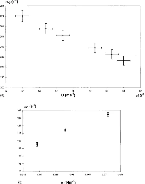
about frequency can be summarized in the following way: ~i! for a given geometry the frequency decreases with the jet velocity@Fig. 4~a!#, ~ii! it increases with surface ten-sion @Fig. 4~b!#, ~iii! when the depth, or U, is varied, the most relevant parameter seems to be the bump height b
8
~where primes denotes quantities related to the bump! as
shown in Fig. 4~b! of @10#.
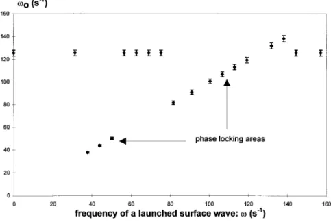
It appears that the jet rotation can be synchronized when excited with surface waves in the range of frequencies cor-responding to the free rotation one. This was shown in a series of experiments, which present some similarities with the oscillating edge experiment by Staubli and Rockwell
@13#. Surface waves were generated on the water tank
through a blade connected to the coil of a loudspeaker. The evolution of the bump oscillation with the forcing frequency has been followed. Two phase-locking areas have been seen for forcing frequencies close to the bump frequency or in a region at lower frequencies. For other frequencies both os-cillations, i.e., forcing waves and bump oscillation coexist
~see Fig. 5!.
C. Discussion
The observed rotation of the bump suggests that the jet is subjected to a helical instability. This is compatible with the Reynolds number range. Moreover, previous works demon-strated that a few diameters away from the nozzle, when the shear layer has widened, this mode is the one with the largest growth rate @11,12#. However, for the free jet, the most un-stable v are of order of 0.5U/b, which corresponds to fre-quencies of the order of 100 Hz for the present experiment, i.e., typically three times the experimental ones. In addition, the observed frequency decreases with jet velocity instead of increasing. An additional frequency-selection mechanism must be invoqued. The water-air interface, which is not in the standard theory, provides this ingredient. The helical in-stability distorts the surface and this causes a pressure fluc-tuation along the jet path, which can be amplified by the jet. Such an amplification is well known and examples are given in @14,15#. Indeed the strength of the feedback will depend on the amplitude of the surface distortion. When the helical instability distorts the bump, surface tension tends to restore the initial shape, which corresponds to the equilibrium be-tween the surface tension and the pressure. The spring force scales as sb
8
, i.e., the product of the surface tension by a characteristic length. To restore the initial shape, this force has to modify the momentum of the water inside the bump, which scales asrU8
b8
3. The characteristic time of the bump relaxation is the ratio of these two quantities, i.e., t5rU
8
b8
2/s. Thus the feedback between the bump and the jet is expected to be optimum when the latter rotates at an angular velocityv0, so thatv0tr51, i.e.,v0 is proportionaltos/rb
8
2U8
.Using the flow rate conservation b
8
2U8
5b2U, the scal-ing of frequency should bev05G(U)s/rb2U, where G(U)is an unknown dimensionless number that takes into account the numerical factor and the actual geometry of the flow, which may vary with the jet velocity. In Fig. 6,rb2Uv0/s
@i.e., the expected G(U)# is plotted as a function of the
ve-locity of the jet for various water velocities and depth. The fact that this quantity is almost constant~except for high U,
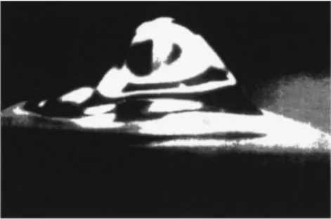
FIG. 2. Picture of a rotating bump for U.Uc. The jet diameter
is equal to 1 mm, the height and width of the bump are of the same order, about 3 mm.
FIG. 3. Picture from above of the surface waves generated by the rotating bump~spiral waves!.
i.e., low v0! shows that the model for oscillation is correct
and moreover that geometry distortion due to variations of U is not too large. In conclusion, taking into account the value of G deduced from Fig. 6 one gets
v05~0.960.1!s/rb2U. ~1!
It is also possible to eliminate U
8
in the relation v0's/rb
8
2U8
using the equilibrium discussed in Sec. II A between the stressrU8
2and superficial tensions/b, i.e., U8
is proportional to b20.5 so that v0 should approximativelyscales with b21.5. This curve is compatible with experimen-tal results @10# although the exponent cannot be determined accurately ~between 22 and 21.5!.
As discussed at the beginning of the section, these fre-quencies are two or three times lower than the optimum for the amplification by the jet. However, taking a reasonable velocity profile across the jet, the linear theory still predicts an instability with Re(kz) and Im(kz) of the order of 1000 and
100 m21, respectively@12#. The amplification takes place on distances l lying between b
8
and h so that its value eIm(kz)1will be in the range 1–1.5. If the coupling between the pres-sure modification due to the bump distortion and the jet is not too lossy, the system can oscillate. To explain the rota-tion start at U5Uc, the following scenario is likely: when U
is low, the Reynolds number is too low for an amplification process to take place. When U increases above Uc, Im(kz)
reaches a value such that the oscillation is possible. The most favored frequency is v0 since the feedback on pressure is optimum at the bump resonance.
The loudspeaker experiment can be interpreted along the same lines. When the incoming waves distorts the bump ef-ficiently i.e., when its frequency is close tov0 it can lock in
phase the jet instability. This is not contradictory with the presence of another region at lower frequency, where there is a phase locking that could correspond to the direct excitation of the jet by the surface wave.
FIG. 4.~a! Evolution ofv0with the jet velocity U. ~b! Effect onv0of a change in surface tension obtained by adding soap to water.
III. COUPLING OF OSCILLATORS IN SIMPLE GEOMETRIES
A. Experimental results with simple arrays
Results of Sec. II suggest that when the system contains several jets, they can be coupled. This has been investigated for two types of jet configurations.
~i! The first one consists in two jets separated by distances
631023,a,1231023m, the plate being 6 mm deep. When a is too large ~above 1231023m! the coupling dis-appears. The flow rate was varied, limited on the lower side by the threshold for jet oscillation, and on the upper side by the fountain regime. This corresponds to the single jet fre-quency range: 240,v0,300 s21@Eq. ~1!#. The two bumps
oscillate at the same frequency, with the same amplitude
~note that the photodiode technique does not allow an
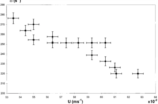
accu-rate amplitude measurement! and the same direction of rota-tion. There are two differences with the single jet case: ~i! the critical flow rate for the bump oscillation appearance is lower for two bumps than the one for a single one, ~ii! the frequencyvis different from the single jet onev0 as shown
in Fig. 7. The results obtained duringv0 scans~i.e., U scans
sincev0 decreases as U increases! for various values of jet spacing a, are presented in Table I. The second column rep-resents the phase difference between the motion of the two jets. Two collective modes are observed: an acoustic mode where the two bumps oscillate in phase~phase difference of 2p!, and an optical mode where the two bumps oscillate in phase opposition ~phase difference of p!. When there is a transition, the symbol at left ~right! represents the mode at low ~high!v0. In this case the value ofv0 at the transition
is displayed in the third column. A transition between two
FIG. 5. Effect on the bump pulsationv0of a launched surface wave~blade connected to a loudspeaker excited by a sinusoidal tension!.
The natural value ofv0is 126 s21.
FIG. 6. Evolution of the rescaled pulsation Y5rv0b2U/s with the jet velocity U for one single jet, for different depths. The figure
modes is accompanied by a phase and frequency jump ~al-ways positive whenv0 increases!, which is indicated in the
last column. Around the transition there is a domain where the system hesitates between the two modes with a typical half-width Dv0510 s21. Similar results are obtained for lines of five jets.
~ii! The second network is made of four jets displayed on
squares of different sizes. The plate is still at 6 mm from the surface. For this network the onset of the threshold velocity is lower than for two jets so that the range ofv0that can be
explored is larger, between 240 and 310 s21. As for the two-jet network, bumps oscillate at the same frequency at quali-tatively the same amplitude and the same direction of rota-tion. The two modes are recovered: in the optical mode the two adjacent jets on the square oscillate in phase opposition while in the acoustic mode all jets are in phase. Again there are transitions and a perturbed area in the transition zone. The results are presented in Table II.
B. Modelization
A natural model to fit the data should be a network of jets oscillating all at the same frequency vwith the same direc-tion of rotadirec-tion and coupled through surface waves. One con-siders first jet m. It is defined by its position Zm5Xm
1iYm, and the bump displacement is zm5xm1iym. When
the stationary state is reached, zm5ameiv0t with am its
slowly varying complex amplitude and fm5arg(am)
repre-sents the phase of the motion. When jet m is alone, the rotation occurs with a pulsation v0 so that the argument of
am does not depend on time. This behavior is well
repre-sented by the following equation: dam
dt 2g~U!~12amam*!am50, ~2!
where an asterisk denotes complex conjugate. The second term represents the effect of the jet instability, which ampli-fies the motion at a rate g,gis real~positive when U.Uc!,
and which saturates foruamu51 ~amplitudes have been
nor-malized to the free jet saturation amplitude!.
One considers now an array of jets, coupled through sur-face waves. This can be more easily studied when the bumps rotate in stationary conditions at the frequency v, i.e., when
am(t)5a0e
i(v2v0)t. Note thatv2v
0!v0 so thatam(t) is
a slowly varying function. Surface waves have a well-defined wave number k(v), which is the solution of the surface wave dispersion relation for deep water@in our case the product k(v)3(depth) is about 5# @16#:
k~v!g1k~v!3gl2c2v250 with lc25s
rg. ~3! A given jet n radiates a spiral capillary wave, which depends on the flow velocity U and on the bump displacement.
Dur-FIG. 7. Evolution of the pulsation for two coupled jets with a511 mm ~squares!, and for one single jet ~circles! as a function of the jet velocity.
TABLE I. Modes in a two-jet array for 240,v0,300 s21.
a (m) Phase difference v0at transition (s21) v jump at transition (s21) 0.006 p→2p 275 220→220180 0.0085 2p→p 280 226→226156 0.009 2p→p 270 226→226156 0.011 p
TABLE II. Modes in a four-jet array for 240,v0,310 s21.
a (m)
Phase difference
~neighboring jets! v0at transition(s21)
v jump at transition
(s21)
0.0085 2p→p 295 250→250140
0.009 p
0.011 p→2p 300 250→250156
ing its propagation between jets n and m separated by a distance rmn, the wave is attenuated by geometrical effect
~energy flux proportional to 1/r in cylindrical geometry! and
other dissipation mechanisms. The total attenuation will be included in a function f (r). The wave experiences also a phase shift given by k(v)rmn. The simplest coupling term in
the amplitude equation compatible with surface waves leads to the following equation:
i@v2v0~U!#am2g~U!~12amam*!am
1l~U!
(
nÞm
f~rmn!e2ik~v!rmna
n50. ~4!
The function v0(U) is the free jet frequency, which can be
measured directly by single jet experiments @see Fig. 4~a!# andvis the frequency of the motion in the array. The cou-pling constant l(U) contains the wave amplitude and the physics of the forcing effect of a wave on the helical jet instability.
This model allows us also to recover the fact that the threshold is lower when there are several jets. For instance, if one considers now in Eq. ~4! a small amplitude oscillation
~instead of a saturated one!, the real part reads
Imv52g~U!1Re
S
l(
nÞm
f~rmn!e2ik~v!rmn
D
50. ~5!Even for U,Ucso thatgis negative, the growth rate can be
positive in accordance with the observations described in Sec. III A.
There are two parameters in our dynamical system:g(U) the growth rate of the free jet instability, the coupling con-stant l(U). In addition, the function f (r) must be adjusted. For the sake of simplicity, it will be taken equal to e2mr. The parameters g,l,mdo not depend on the geometry of the jet lattice~a dependence in the nozzle diameter and depth is not excluded but all experiments have been made taking these two parameters constant!. In Sec. III D, experiments will be simulated fitting g(U), l(U), and m by simple number. Thus the parametersl andgwill be taken independent of U, i.e., the notation ‘‘function of U’’ will be skipped.
C. Analytic determination of phase patterns of two- or four-jet arrays
1. Two-jet network
The system is described by a set of two equations, which admit obviously solutions with uz1u5uz2u5uau. A mode is
defined by the phase shift between both jets Df5f22f1.
The system~4! becomes
i~v2v0!uau2g~12uau2!uau1le2mae2ik~v!auaueiDf
50, ~6a!
i~v2v0!uau2g~12uau2!uau1le2mae2ik~v!auaue2Df
50. ~6b!
This system has solutions if Eqs.~6a! and ~6b! have the same
v as solution. Two modes are allowed, Df50 or Df5p. Their frequencies and amplitudes are obtained from the real and imaginary parts:
v«2v01«ulue2ma Im@ei@2k~v!a1arg~l!##50, ~7a!
2g~12ua«u2!1«ulue2ma Re@ei@2k~v!a1arg~l!##50
~7b!
with« equal to 21 or 1, respectively, for the optical and the acoustic mode. From Eq. ~7a! it is possible to deduce the frequency and amplitude of both modes. A simple approxi-mation can be obtained using v«2v0!v0, i.e., taking the
coupling terms evaluated for v5v0:
FIG. 8. Functionsv«(v0) anda«(v0) defined by Eq.~8!;
dot-ted line ~acoustical mode!, full line ~optical mode!. The numerical values chosen here are a58.5 mm and le2ma515e23ip/4.
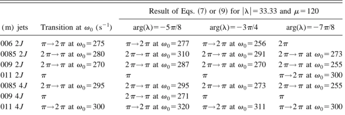
TABLE III. Experimental modes and simulated ones for three values of arg~l!.
a (m) jets Transition atv0(s21)
Result of Eqs.~7! or ~9! for ulu533.33 andm5120
arg(l)525p/8 arg(l)523p/4 arg(l)527p/8
0.006 2J p→2p at v05275 p→2p at v05277 p→2p at v05256 2p 0.0085 2J 2p→p at v05280 2p→p at v05310 2p→p at v05291 2p→p at v05273 0.009 2J 2p→p at v05270 2p→p at v05287 2p→p at v05270 2p→p at v05255 0.011 2J p p p p→2p at v05300 0.0085 4J 2p→p at v05295 2p→p at v05295 2p→p at v05273 2p→p at v05255 0.009 4J p 2p→p at v05271 p p 0.011 4J p→2p at v05300 p→2p at v05320 p→2p at v05311 p→2p at v05300
v«5v02«ulue2masin@2k~v0!a1arg~l!#, ~8a!
ua«u2512
«
g ulue2ma cos@2k~v0!a1arg~l!#. ~8b!
Forv0, i.e., U values so that2k(v0)a1arg(l)5p/2~mod
p!, the two modes have the same amplitude ~equal to 1!. At
these points the frequency difference between the two modes is 2ulue2ma. In the Appendix it is shown that only the mode that has the largest amplitude is stable. This means that ex-perimentally only this mode should be seen. An example of this prediction is shown in Fig. 8, which illustrates one of the computations discussed in Table III. The functions a«(v0)
andv«(0) are shown for a58.5 mm and l515e23ip/4. Ac-cording to the prescription that the observed mode is the one with the largest amplitude, a jump from acoustic to optical mode should be observed atv0 around 275 s21.
2. Four-jet network
One considers now a network with four jets on a square. Introducing the experimental mode structure, i.e.,@0000# and
@0p0p# in Eq. ~4!, one obtains the equation equivalent to Eq.
~7!:
~v«2v0!1uluIm~2«e2mae2ik~v!a1i arg~l!
1e2ma&e2ik~v!a&1i arg~l!)50, ~9a!
2g~12ua«u2!1uluRe~2«e2mae2ik~v!a1i arg~l!
1e2ma&e2ik~v!a&1i arg~l!!50, ~9b! with « equal to 1 or 21, respectively, for the acoustic and the optical mode. These equations provide the evolution of the amplitude and the frequency of each mode with the natu-ral frequency v0. Again, within the approximation v«2v0
!v0, the two modes have the same amplitude for
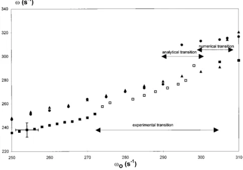
FIG. 9. Pulsation of the motion of jets displayed on a square (a511 mm) as a function of the free jet pulsation (v0). Experimental
results for a depth56 mm ~squares!, solution of Eq. ~8! ~circles!, numerical simulation ~triangles!, withm5120, g560, l533.3e2i33p/4. The lines with double arrows on the graph represent the transition areas between the acoustic and the optical mode.
TABLE IV. Mode transitions for three values ofulu andm and arg(l)523p/4.
a (m) number of jets
Experimentalv jump (s21)
Solution of Eqs.~7! ~two jets! or ~9! ~four jets!
ulu560 m550 ulu5100m5120 um5250lu5320 0.006 2J 220→220180 230→230170 220→220180 210→210190 atv05275 s21 atv05255 s21 atv05255 s21 atv05255 s21 0.0085 2J 226→226156 250→250155 250→250160 250→250160 atv05280 s21 atv05293 s21 atv05290 s21 atv05291 s21 0.009 2J 226→226156 240→240155 240→240165 240→240160 atv05270 s21 atv05270 s21 atv05270 s21 atv05269 s21 0.0085 4J 250→250140 250→250190 240→240180 230→230180 atv05295 s21 atv05262 s21 atv05258 s21 atv05258 s21 0.011 4J 250→250156 250→250190 260→260190 260→260180 atv05300 s21 atv05310 s21 atv05310 s21 atv05312 s21
2k(v0)a1arg(l)5p/2~modp!, while the frequency
differ-ence at the transition between the two modes is 4ulue2ma.
IV. COMPARISON WITH THE EXPERIMENTAL DATA A. Mode transition
In Table III, one shows a comparison between the experi-mental data and the ones obtained with the analytical treat-ment for values of arg(l) in an optimum range, i.e., around
23p/4. The second column of Table III contains experimen-tal data from Sec. III A while the last three columns give the modes with the largest amplitudes obtained from Eqs.~7! or
~9!. arg(l) has been determined by trying to fit all the
ob-served transitions~their location depends on ulu only through corrections of order (v2v0)/v0, as can be seen in Table
IV!, or at least the observed modes when the values of jet spacing a correspond to windows without transition. The computations are made in the window 250,v0,325 s21for
two and four jets. The predicted modes are in quite good agreement with the experimental ones, especially if one takes into account the error bars about1/210 s21onv0 at
tran-sition. In the following arg(l)523p/4 will be taken. B. Strength of the coupling
In a second step,ulu andmcan be found from expression
~7a! using the two-jet experiment. For both modes,
experi-mental frequencies should follow the relation
ln
U
v22v 0 2
cos„k~v!a1p/4…
U
5lnulu2ma. ~10! If the value of v can be measured as a function of a, it should be possible to guess ulu andm. However, due to the small range of a and the low value of attenuation, the accu-racy is poor. Several combinations of l andm are possible providedulue2amstays in the same range. This is shown in Table IV, which displays a comparison between the five ex-perimental mode transitions given in Tables I and II and the simulated ones taking two combinations ofulu andm.To summarize, from Tables III and IV, it appears that the amplitude, nature, and location of modes can be reasonably fitted by the model especially if one takes into account the small number of parameters to be fitted: One @arg(l)# to fit all the transition ~location and direction! and two @modu-lus~l! andm# for the values of frequencies ~with little effect!. The value ofgplays almost no role~it has been taken equal to 60!. An example of comparison theory-experiment of
v(v0) for a four-jet system is shown in Fig. 9. The transition
has been simulated in two ways. First there is the largest amplitude mode given by Eq. ~9!. One admits then that the system cannot choose between the two modes if it exists a difference of less than 10% between the amplitudes of the modes. This assumption allows us to determine a small tran-sition zone ~‘‘analytical transition’’! where the two modes, like in the experiments, are unstable. This is possibly due to desynchronization as discussed in the next section. Second, there is the result obtained by evolving in time the jet motion using a scheme described elsewhere@17#.
C. Effect of a scattering of oscillator properties When a increases beyond 12 mm, the synchronization becomes poor and eventually is lost. Another experimental feature is that, in the transition zone~when the amplitudes of the two modes are close together! the system is unstable. A possible explanation could be the unavoidable dispersion in the v0 values, which tends to hamper the synchronization.
This is a well known effect for coupled oscillators @1#. This effect has been investigated more quantitatively for a two-jet system. One assumes that there is some scatter in the v0
values, i.e., that they become v1,25v06D. In the presence of coupling, the motion of jet m can be expressed as
am(t)e2iv0
t. Provided it is slowly varying, the evolution of
am(t) obeys the following equation:
dam dt 2i~vm2v0!am2g~12amam*!am 1l
(
nÞm e2mae2ik~vn!rmna n50. ~11!Equation ~11! has been solved using an iterative scheme to determine the vn values to be used in the coupling
coeffi-cients@17#. For the system chosen ~a58.5 mm as in Fig. 8! there is a predicted transition acoustic→optical at v0
5291 s21~observed at 280 s21!. For D50, these modes are found by the evolutive computation. When D is nonzero, depending on the le2ma value, there exists a zone D
,Dmax where a synchronization is possible. The value of
Dmaxdepends on k(v0)a1arg(l) and ule2mau. This domain
is displayed in Fig. 10~a! for v05240 s21 ~far from the
mode transition! and 295 s21 ~close to the mode transition!. The synchronization domain depends on k(v0)a, i.e., the
phase of the interaction between the jets. In particular, close to the transition point, the system becomes very sensitive to any defect, i.e., is hard to synchronize. This is expected since at this location the eigenvalues associated to the mode sta-bility analysis are close to zero ~see the Appendix!. This is shown in Fig. 10~b!, which displays the value of Dmax for
ule2mu515 as a function ofv
0. This simple model explains
two experimental findings.~i! The synchronization becomes difficult for a.12 mm. According to Table IV, the values of
le2ma at this point range between 16 (m5120) and 32 (m
550). For such coupling parameters, according to Fig.
10~b!, the desynchronization occurs for D about 10– 20 s21, i.e., anv0 scatter in the range 5–10 %, i.e., according to Eq.
~1! a scatter in the hole diameter of order of 5%. ~ii! The
width of the unstable domain in Fig. 10~b! is compatible with the width of the transition zone in experiments.
V. CONCLUSION
The mechanism for the oscillation of a single vertical jet impinging on an interface has been investigated. It turns out that a feedback mechanism between surface waves and the unstable jet is at the origin of the oscillations of the bump to the surface. An analogy can be made with the ‘‘jet-edge’’ system if considering a ‘‘resonant edge’’ mechanically at-tached to springs. Indeed, the stiffness of the springs is here equivalent to the surface tension of the fluid. In a dimen-sional model, the frequency is found to be proportional to the
surface tension and conversely proportional to the jet veloc-ity. These results are in good agreement with the experimen-tal results obtained when varying the surface tension of the fluid, the velocity of the jet, and the depth of the nozzle.
Considering simple ensembles of jets, a phase-locking mechanism has been observed. When the jet velocity, i.e., the resonant frequency is modified and two modes are ob-served, namely an acoustic mode and an optical one. A mod-elization in which each bump is a nonlinear oscillator coupled with its neighbors through surface waves gives rea-sonable agreement with the experimental results, especially if one takes into account the scatter of jet frequencies due to imperfections. Generalization of this model to infinite net-works is possible at the expense of a more complex formal-ism, which will be presented in a forthcoming paper@17#. It appears that systems of jets are very close to the large popu-lation of coupled oscillators investigated by theoreticians. There is, however, one important difference, the coupling is ensured not by instantaneous interaction~reflected by a cou-pling constant! but by traveling waves propagating at finite velocity. This plays a significant role in the formation of phase patterns observed in large regular networks.
APPENDIX: STABILITY ANALYSIS OF THE LIMIT CYCLE IN THE TWO JET CONFIGURATION Following the notation of Sec. III C, the two jet system has two limit cycles described by Eq.~6!, the acoustic mode with an amplitude at saturation a1 and a frequencyv1 and the optical mode with an amplitude a21 and a frequency
v21. The phase shift between the bumps of a given mode is
f«, which is equal to zero for«51 and p otherwise. The equations governing the eigenmodes are
i~v«2v0!2g~12a«a«*!1le2ma2ik~v«!aeif«50.
~A1!
One considers that the system is at the limit cycle for the mode « ~51 or 21! so that the envelope of rotation of bump m (m51,2) is close to a«ei(v«2v0)t1imf«. A small perturbation corresponding to a mode «
8
Þ« is added which is of the form f (t)ei(v«82v0)t1imf«8. Thus, the envelope of the position of bump m is am5a«e@i(v«2v0)t1imf«#1 f (t)ei(v«82v0)t1imf«8and is as follows:
dam
dt 2g~12amam*!am1le2ma2iv0t@e2ik~v«!aa«ei~v«t1f«!
1e2ik~v«8!af~t!ei~v«8t1f«8!#50. ~A2!
The zero-order equation gives the equation of the limit cycle of mode«. The terms can then be developed to first order in f . The linearized terms are
dam dt →
S
d f dt1i~v«8
2v0!f ~t!D
e i~v«82v0!t1imf«8, amam*am→a« 2ei~v«82v0!t1imf«8@2 f ~t!1 f*~t!e2iu~t!# withu(t)5(v«2v
8
«)t1m(f«2f«8).After multiplication by e2iv«8t2imf«8, an evolution equa-tion for f (t) can be deduced from the linearized equaequa-tion
~A1!,
d f
dt1i~v«
8
2v0!f ~t!2gf~t!12ga«2
f~t!
1l f~t!e2mae2ik~v«8!a1if«852ga «
2
f*~t!e2iu~t!.
~A3!
Using Eq.~A1! expressed for the limit cycle of mode «
8
, Eq.~A3! can be simplified. Taking the complex conjugate, a
similar equation can be obtained for f*(t),
d f gdt5~a«8 2 22 a«2!f ~t!2a « 2f *~t!e2iu~t!,
FIG. 10. ~a! Synchronization domain forv05240 s21~crosses!
and 295 s21 ~stars! for a two-jet system with a58.5 mm in the space X5ule2mu and Y5D; @arg(l) is kept equal to 23ip/4#. ~b! Value of Y5Dmaxas a function of X5v0forle2m515e23ip/4and
a58.5 mm.
d f* gdt52a« 2f~t!e22iu~t!1~a «8 2 22 a«2!f*~t!.
Since u(t) is a slowly varying function, the system can be considered as a linear operator on f . The eigenvalues l are
given by the zeros of the determinant l222l(a« 8 2 22 a«2) 1(2a«22a «8 2 )22a «
4. The roots are a
«8 2 23 a«2 anda «8 2 2 a«2.
Both roots have a negative real part, i.e., the system is stable if and only if the limit cycle corresponds to the mode with the largest amplitude.
@1# P. C. Matthews, R. E. Mirollo, and S. H. Strogatz, Physica D 52, 293~1991!.
@2# N. Nakagawa and Y. Kuramoto, Prog. Theor. Phys. 89, 313 ~1993!.
@3# V. Hakim and W.-J. Rappel, Phys. Rev. A 46, 7347 ~1992!. @4# P. Legal, M. P. Chauve, I. Peshard, and S. Jarre, Curr. Top.
Phys. Fluids Res. Trends 1, 307~1994!; I. Peshard and P. Le Gal, Phys. Rev. Lett. 77, 3122~1996!.
@5# E. Villermaux and E. J. Hopfinger, Physica D 72, 230 ~1994!;
J. Fluid Mech. 263, 63~1994!.
@6# H. Willaime, O. Cardoso, and P. Tabeling, Phys. Rev. Lett. 67,
3247~1991!.
@7# E. Villermaux, Phys. Rev. Lett. 75, 4618 ~1995!.
@8# A. Maurel, S. Cremer, and P. Jenffer, Europhys. Lett. 39, 503 ~1997!.
@9# S. Houard, F. Daviaud, and P. Berge´, Europhys. Lett. 32, 101 ~1995!.
@10# S. Houard, F. Daviaud, and P. Berge´, Physica D 99, 318 ~1997!.
@11# G. E. Mattingly and C. C. Chang, J. Fluid Mech. 65, 541 ~1974!.
@12# P. J. Morris, J. Fluid Mech. 77, 511 ~1976!.
@13# A. Powell, J. Acoust. Soc. Am. 33, 395 ~1961!; D. Rockwell
and E. Naudascher, Annu. Rev. Fluid Mech. 11, 67~1979!; D. G. Crighton, J. Fluid Mech. 234, 361~1992!.
@14# S. M. Kusek, T. C. Corke, and P. Reisentel, Exp. Fluids 10,
116~1990!.
@15# T. Staubli and D. Rockwell, J. Fluid Mech. 176, 135 ~1987!. @16# L. D. Landau and E. M. Lifshitz, Fluid Mechanics ~Pergamon,
Oxford, 1987!.