HAL Id: hal-02923452
https://hal.archives-ouvertes.fr/hal-02923452
Submitted on 27 Aug 2020
HAL is a multi-disciplinary open access archive for the deposit and dissemination of sci-entific research documents, whether they are pub-lished or not. The documents may come from teaching and research institutions in France or
L’archive ouverte pluridisciplinaire HAL, est destinée au dépôt et à la diffusion de documents scientifiques de niveau recherche, publiés ou non, émanant des établissements d’enseignement et de recherche français ou étrangers, des laboratoires
Ambiguity Preferences and Portfolio Choices
Milo Bianchi, Jean-Marc Tallon
To cite this version:
Milo Bianchi, Jean-Marc Tallon. Ambiguity Preferences and Portfolio Choices: Evidence from the Field. Management Science, INFORMS, 2019, 65 (4), pp.1486-1501. �10.1287/mnsc.2017.3006�. �hal-02923452�
« Toulouse Capitole Publications » est l’archive institutionnelle de l’Université Toulouse 1 Capitole.
“Ambiguity Preferences and Portfolio Choices: Evidence
from the Field”
Milo Bianchi and Jean‐Marc Tallon
‐
Ambiguity Preferences and Portfolio Choices: Evidence
from the Field
Milo Bianchi and Jean‐Marc Tallon
November
Ambiguity Preferences and Portfolio Choices:
Evidence from the Field
Milo Bianchiy Jean-Marc Tallonz
November 2017
Forthcoming in Management Science
Abstract
We match administrative panel data on portfolio choices with sur-vey data on preferences over ambiguity. We show that ambiguity averse investors bear more risk, due to a lack of diversi…cation. In particu-lar, they exhibit a form of home bias that leads to higher exposure to the domestic relative to the international stock market. While more sensitive to market factors, their returns are on average higher, sug-gesting that ambiguity averse investors need not be driven out of the market for risky assets. We also show that these investors rebalance their portfolio more actively and in a contrarian direction relative to past market trends, which allows them to keep their risk exposure rel-atively constant over time. We discuss these …ndings in relation to the theoretical literature on portfolio choice under ambiguity.
We are grateful to Han Bleichrodt (editor), an associate editor and two referees for very constructive comments. We also thank Marianne Andries, Luc Behaghel, Bruno Biais, Luigi Guiso, Roy Kouwenberg, David Margolis, David Schroeder, Bernard Salanié, Paul Smeets, Vassili Vergopoulos, Peter Wakker and various seminar participants for very useful discussions, and Henri Luomaranta for excellent research assistance. Financial support from AXA Research Fund and from the Amundi, Groupama and Scor Chairs is gratefully acknowledged.
yToulouse School of Economics, University of Toulouse Capitole, Toulouse, France.
E-mail: milo.bianchi@tse-fr.eu
1
Introduction
Ambiguity has been widely studied both theoretically and experimentally in the past decades. Its implications have been investigated in a variety of settings, including …nancial behaviors.1 It is now commonly understood, at least at an intuitive level, that ambiguity is an important element that house-holds face in their …nancial decisions (Ryan, Trumbull and Tufano (2011), Guiso and Sodini (2013)). It may also be a key ingredient to explain the functioning of …nancial markets.2 Field evidence of how ambiguity a¤ects households is however still very scarce:
Interestingly, the empirical literature has so far provided little ev-idence linking individual attitudes toward ambiguity to behavior outside the lab. Are those agents who show the strongest degree of ambiguity aversion in some decision task also the ones who are most likely to avoid ambiguous investments? (Trautmann and Van De Kuilen (2015))
This paper attempts to partially …ll this gap. We explore the relation between ambiguity aversion and portfolio choices using a unique data set that matches administrative panel data on portfolio choices with survey data on preferences over ambiguity.
We have obtained portfolio data from a large …nancial institution in France. We focus on a popular investment product among French house-holds dubbed assurance vie. In this product, househouse-holds decide their portfo-lio weight on relatively safe assets (essentially bundles of bonds, called euro funds) vs. relatively risky assets (essentially mutual funds, called uc funds) as well as some features of risky assets (such as their exposure to the do-mestic vs. international stock markets). Households can freely change their portfolios over time. Our data record the clients’ portfolio of these contracts at a monthly frequency for about nine years. Moreover, for each portfolio, we can construct the corresponding returns.
Clients were also asked to answer a survey that we have designed and that serves two main purposes. First, while portfolio data only concern house-holds’ activities within the company, in the survey we gather a more
com-1See, e.g., Etner, Jeleva and Tallon (2012), Machina and Siniscalchi (2014), Gilboa and
Marinacci (2013) for surveys of the various models, and Hey (2014) or Trautmann and Van De Kuilen (2015) for surveys of the experimental literature. Closely related experimental evidence is provided in Ahn, Choi, Gale and Kariv (2014), who study how ambiguity aversion a¤ects portfolio choices, and in Bossaerts, Ghirardato, Guarnaschelli and Zame (2010), who focus on its e¤ects on asset prices.
2Epstein and Schneider (2010) and Guidolin and Rinaldi (2013) provide recent
insight-ful reviews on ambiguity and …nancial choices. Macro-…nance applications include Uppal and Wang (2003), Ju and Miao (2012), Collard, Mukerji, Sheppard and Tallon (2012). On the role of ambiguity in …nancial crises, see e.g. Caballero and Krishnamurthy (2008) and Caballero and Simsek (2013).
plete picture of households’ portfolios as well as various socio-demographic data. Second, we elicit a number of behavioral traits, and in particular households’ attitudes towards ambiguity. Following standard procedures, we build our main measure of ambiguity aversion by asking subjects to choose between lotteries with known vs. unknown probability distributions over the …nal payo¤s.
Guided by some fundamental insights developed in the theoretical lit-erature of portfolio choices under ambiguity, we focus on three dimensions of household portfolios. We …rst look at how the composition of portfo-lios varies with ambiguity aversion. Is it the case that ambiguity aversion leads to a form of under-diversi…cation, as predicted for example in Uppal and Wang (2003) and Hara and Honda (2016)? In particular, do ambiguity averse investors display a preference for home stocks, as in Boyle, Garlappi, Uppal and Wang (2012)?
Second, we ask whether ambiguity averse households display distinct portfolio returns. Are their returns systematically lower, so that in the long run these investors are bound to be wiped out of the market, as in Condie (2008)? At the same time, in relation to under-diversi…cation, are their returns more volatile?
Third, we analyze the relation between ambiguity aversion and portfolio dynamics. In particular, as suggested by recent models on portfolio inertia (Garlappi, Uppal and Wang (2007), Illeditsch (2011)), is it the case that ambiguity averse households keep their portfolio weights more stable over time?
In terms of portfolio composition, we …nd that ambiguity averse investors are more exposed to risk, as de…ned both in terms of the volatility of returns and in terms of beta relative to the French stock market. This extra expo-sure to risk could come, as suggested for instance by Klibano¤, Marinacci and Mukerji (2005), from a desire to shy away from ambiguity. To pursue this line, we distinguish portfolios according to their relative exposure to the French and the world markets. We build a measure of di¤erential expo-sure based on the di¤erence between a "domestic" beta -which employs as benchmark the French stock market index CAC40- and an "international" beta -which instead uses as benchmark the MSCI World Index. We show that ambiguity averse investors are relatively more exposed to the French than to the international stock market. Ambiguity aversion is thus a good candidate to explain home bias in equity markets.
We also study the extent to which portfolio returns are explained by simple asset pricing models, and in particular by a domestic CAPM and by the Fama-French …ve-factor model. In both speci…cations, we …nd that the higher ambiguity aversion, the lower is the explanatory power of mar-ket factors. Ambiguity averse investors appear to bear more idiosyncratic volatility, suggesting a possible under-diversi…cation in their portfolios.
We then look at portfolio returns. We …nd that, in our sample, ambigu-ity averse investors experience higher returns, even controlling for standard measures of risk. At the same time, however, their returns are more sensitive to market trends. Our estimates show that the larger ambiguity aversion, the higher are returns in good times and the lower are returns in bad times. A similar picture emerges as we explore the di¤erential exposure of am-biguity averse investors to Fama-French factors. These investors experience relatively higher returns when returns of the market portfolio are high, even more so when we construct market returns based only on the French stock market. Moreover, we show that ambiguity averse investors are more ex-posed to the Fama-French investment factor; that is, their portfolios load more on …rms with "conservative" as opposed to "aggressive" investment strategies.
Finally, we investigate the dynamics of household portfolios. In partic-ular, we focus on how households’ risky share, as measured by the share of uc funds in their portfolios, evolves over time. Following the methodology developed in Calvet, Campbell and Sodini (2009), we distinguish changes in risk exposure which are driven by di¤erential returns of risky vs. riskless assets from those which result from an active choice of the household. We show that ambiguity averse investors tend to rebalance their portfolio more actively; that is, their risky share tends to remain closer to the target share. Furthermore, we show that ambiguity averse investors adopt a contrarian strategy, moving wealth from funds which have experienced relatively higher returns to those who had relatively lower returns. This rebalancing strategy aims at keeping the risky share relatively constant over time, which is in line with the above mentioned models of ambiguity aversion and portfolio inertia.
In the next sections we discuss each of these …ndings and we highlight in more details their relation with the existing theoretical literature. From a somewhat broader perspective, we believe these insights contribute to a bet-ter understanding of the empirical content of ambiguity preferences. While from a conceptual viewpoint the importance of ambiguity has been recog-nized at least since Knight (1921), its empirical content is still unclear. In his Nobel lecture, Hansen (2014) calls for further research aimed at assessing whether ambiguity, in addition to risk, is empirically relevant for the study of asset pricing. Our results are strongly suggestive that ambiguity aversion is an important determinant of observed …nancial outcomes. We believe they should serve as motivation for further work aimed at distinguishing more clearly risk from ambiguity both in investors’ perceptions and in their …nancial behavior.
Related Literature
To our knowledge, this study is the …rst to provide evidence on the e¤ect of ambiguity aversion on …nancial outcomes observed in administrative data. As such, it relates, from an empirical angle, to the mostly theoretical liter-ature that has studied the implications of ambiguity aversion for portfolio choices and …nancial markets.3
We also contribute to the household …nance literature by looking at the determinants of households’ …nancial decisions. The literature is growing rapidly and we refer to Campbell (2006) and Guiso and Sodini (2013) for recent surveys. Compared to this literature, our main novelty is in matching survey and administrative data. While as pointed out our data do not pro-vide a detailed picture of the entire households’ portfolios (as for example in Calvet, Campbell and Sodini (2007) and Calvet et al. (2009)), they o¤er the opportunity to study the relation between behavioral traits and the choices taken within the company. The latter allows us to address quantitative issues that purely survey data usually cannot address.
We know of only a few studies combining survey and administrative data. Dorn and Huberman (2005) focus on the relation between risk aversion, (perceived) …nancial sophistication and portfolio choices; Alvarez, Guiso and Lippi (2012) analyze the frequency with which investors observe and trade their portfolio; Guiso, Sapienza and Zingales (2017) and Ho¤mann, Post and Pennings (2013) study how risk aversion has changed following the …nancial crisis; Bauer and Smeets (2015) and Riedl and Smeets (2014) investigate how social preferences a¤ect socially responsible investments. None of these studies focuses on ambiguity preferences as we do.
Most closely related to our study, Dimmock, Kouwenberg and Wakker (2016) and Dimmock, Kouwenberg, Mitchell and Peijnenburg (2016) exploit large representative surveys in which subjects are asked about their prefer-ences over ambiguity as well as about their portfolio holdings. We share with these authors a similar methodology to elicit ambiguity aversion (although our subjects receive no monetary reward in relation to their choices) but the nature of our data, and so the questions we address, are quite di¤erent. Their data are based on surveys, and they are larger in size and in scope. This allows them to investigate issues of stock market participation which we cannot address. Our data provide more details on the investment prod-uct at hand as well as a panel strprod-ucture, and this allows us to investigate questions on portfolio dynamics and returns which cannot be addressed with their data.
Dimmock, Kouwenberg, Mitchell and Peijnenburg (2016) also point at
3Recent developments include Gollier (2011) on the comparative statics of ambiguity
aversion in portfolio choices; Maccheroni, Marinacci and Ru¢no (2013) on mean-variance preferences; Hara and Honda (2016) on CARA smooth ambiguity preferences; Epstein and Ji (2013) and Lin and Riedel (2014) on dynamic portfolio choices.
a positive relation between ambiguity aversion and lack of portfolio diver-si…cation. We complement their …ndings by documenting forms of under-diversi…cation starting from information about realized portfolio returns as opposed to stock holding. This allows to highlight how under-diversi…cation a¤ects the riskiness of household portfolios, and to provide support for the idea that ambiguity averse investors tend to bear more risk so as to avoid ambiguity, consistently with di¤erent models in the literature (see Section 4 for details).
2
Data
We exploit three sources of data. First, we have obtained data on portfolio choices from a large French …nancial institution. These data describe clients’ holdings of assurance vie contracts. These are investment products widely used in France; they are the most common way through which households invest in the stock market.4 A typical assurance vie contract establishes the types of funds in which the household wishes to invest and the amount of wealth allocated to each fund.
A …rst key distinction is between euro funds and uc funds. The …rst type of assets, which are called euro funds, are basically bundles of bonds. The capital invested in these funds is guaranteed by the company. The second type of funds are called uc funds, and they are essentially bundles of stocks. It is made clear to investors that uc funds tend to provide larger expected returns and larger risk. Investors do not observe the exact composition of these funds (neither do we), but they receive some information about the intended risk pro…le of these funds (e.g. conservative vs. aggressive) as well as an indication of their exposure to di¤erent markets. A particularly salient feature is whether funds invest in domestic, emerging, or world markets.
Over time, clients are free to change the composition of their portfolios, make new investment and withdraw money as they wish.5 Investors may opt for automatic rebalancing of their portfolio according to some pre-speci…ed rule. In our sample, less than 10% of investors have chosen this option (see the Online Appendix for further details).
Our portfolio data records at a monthly frequency the value and compo-sition of these contracts for 511 clients from September 2002 to April 2011. These data are combined with the responses to a survey we have designed
4According to the French National Institute for Statistics, 41% of French households
held at least one of these contracts in 2010. This makes it the most widespread …nancial product after Livret A, a saving account whose returns are set by the state. See INSEE Premiere n. 1361 - July 2011 (http://www.insee.fr/fr/¤c/ipweb/ip1361/ip1361.pdf).
5A speci…c feature of the product is that there is some incentive not to liquidate the
contract before some time (8 years in our sample period) so as to take advantage of reduced taxes on capital gains. We show in the Online Appendix that this feature is immaterial for our results.
and which was administered by a professional survey company at the end of 2010:6
The …nancial institution has provided to the survey company a sample of clients who had an account open at the end of 2010. The survey was then implemented in order to obtain a representative sample of French households in terms of family status, employment status, sector of employment, revenues (these characteristics follow o¢cial classi…cations of the National Institute for Statistics).7 All clients in our sample held some assurance vie contract in the …nancial company at the time when the survey was conducted, but not necessarily throughout the entire sample period.8
These contracts can represent a sizeable fraction of households’ …nan-cial wealth. In our sample, the average value of a portfolio is 32; 700 euros, the maximum is 590; 000 euros. The median total wealth in our sample is between 225 and 300 thousand euros and the median …nancial wealth is between 16 and 50 thousands euros. These …gures are in line with those ob-tained for the general French population (see Arrondel, Borgy and Savignac (2012)).9
The survey serves two main purposes: …rst, we have gathered information about demographic characteristics, wealth and portfolio holdings outside the company. In this way we can control for a richer set of clients’ characteristics than those recorded by the company. Moreover, this allows to gauge whether the behaviors we observe within the company are informative for clients’ behaviors in their overall portfolio (see the Online Appendix for details).
A second purpose of the survey is to get an idea of clients’ behavioral characteristics, and in particular of their preferences over ambiguity. In the next section, we describe how we have elicited these preferences.10
Finally, we collected data on portfolio returns. We have obtained from Thomson Reuters Datastream the returns experienced in a given month by
6It was made clear to the subjects that they were contacted as part of a scienti…c
project on risk, while the insurance company was never mentioned during the interview. Clients completed the survey over the internet while on line with the surveyor.
7The insurance company gave to the survey company a sample of approximately 30,000
clients. This sample was strati…ed according to geographic regions (Ile De France, North-East, West, South-North-East, South-West) and the survey was conducted so as to meet pre-speci…ed quotas of respondents in terms of the above-mentioned socio-demographic char-acteristics.
8We did not impose any minimal holding period to be included in the sample. We
discuss in the Online Appendix a series of robustness checks to address the possibility of survivorship bias in this sample.
9For o¢cial and comprehensive data, see the 2010 Household
Wealth Survey from the French National Institute for Statistics
(http://www.insee.fr/en/methodes/default.asp?page=sources/ope-enquete-patrimoine.htm).
1 0Our measure of ambiguity aversion is taken just at one point in time, towards the
end of the sample period. In the Online Appendix, we show that the e¤ects of ambiguity aversion would be similar if we were to restrict our analysis to the beginning of the sample period. This suggests that our measure of ambiguity aversion has a persistent component.
each fund and, based on those, we can build the corresponding returns of each contract.
3
Ambiguity Preferences
We elicit preferences over ambiguity in a classical way. We ask respondents to choose between a risky lottery and an ambiguous lottery. For the former lottery, we provide an exact probability distribution over the …nal payo¤s; for the latter, we provide no information about the probabilities associated to the …nal payo¤s. Depending on their answer, we sequentially provide alternative lotteries in which the risky lottery is made relatively more or less attractive. We describe these lotteries in details in the Appendix.
This approach is in line with the results in Dimmock, Kouwenberg and Wakker (2016), who formally show that ambiguity attitudes can be entirely described by matching probabilities. Di¤erently from Dimmock, Kouwen-berg and Wakker (2016), we only had space for a few questions and thus we could only construct a coarser measure of ambiguity attitudes. More-over, our lotteries were hypothetical, and this comes with the usual pros and cons.11 As we detail below, however, we have found a remarkable con-sistency across various measures and elicitation methods, which suggests we are capturing a systematic component of investors’ preferences.
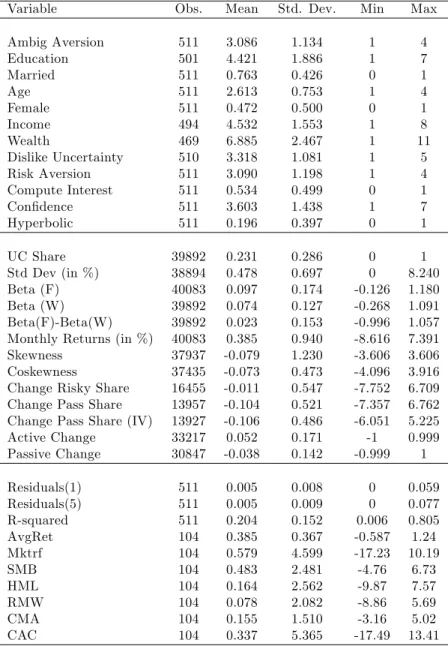
We build the index Ambig Aversion which takes value 1 to 4 from the least to the most ambiguity averse client. This variable will serve as our main measure of ambiguity preferences.12 In the Appendix, we also provide a description of the other variables used in the subsequent analysis. In Table 1, we report some descriptive statistics.
We …rst explore the correlation between Ambig Aversion and a set of demographic characteristics: age, gender, education, marital status, income, wealth (we refer to Table 1 in the Online Appendix for the corresponding results). Ambig Aversion appears negatively related to age and positively related to income. Other variables are not signi…cantly correlated.13 We also observe that our index is positively related to a qualitative measure of ambiguity aversion, which is based on how much the subject declares disliking uncertainty.
We then analyze the relation between ambiguity aversion and other be-havioral traits. We start with risk aversion. Existing results on the
rela-1 rela-1See Dimmock, Kouwenberg and Wakker (2016) and Gneezy, Imas and List (2015) for
a discussion.
1 2In the Online Appendix, we consider several alternative measures such as dummy
variables coding subjects as ambiguity averse as well as accounting for preferences in the loss domain.
1 3Butler, Guiso and Jappelli (2014) …nd a strong positive relation between ambiguity
aversion and wealth. In our data, the relation is positive but not precise (t-stat 1.63). It would be interesting for future studies to explore this relation more systematically.
tion between risk and ambiguity preferences are not conclusive: Dimmock, Kouwenberg and Wakker (2016) report a negative relation while Butler et al. (2014) a positive relation between the two (see Wakker (2016) for an exhaus-tive list of references). We build a 1 to 4 index Risk Aversion (1 being the least and 4 the most risk averse client) by asking respondents to compare a sure outcome to a series of risky lottery. We observe no signi…cant relation between risk and ambiguity aversion in our sample.
The literature suggests that ambiguity preferences may also relate to other characteristics such as sophistication (Halevy (2007); Chew, Ratch-ford and Sagi (2017)), lack of con…dence about the context (Heath and Tversky (1991); Fox and Tversky (1995)), or present biased preferences (Halevy (2008); Cohen, Tallon and Vergnaud (2011)). Our survey allows to build some measures related to these traits, as we detail in the Appendix. We observe no signi…cant relation between Ambig Aversion and our mea-sures of sophistication, con…dence, and time preference. This suggests that, in our subsequent analysis, these behavioral traits are unlikely to interfere with the estimated e¤ects of ambiguity aversion.14
4
Portfolio Composition
In this section, we investigate how ambiguity aversion a¤ects the composi-tion of household portfolios. We …rst revisit some theoretical insights on this relation. We then provide evidence that ambiguity averse decision makers are more exposed to domestic risk, in line with the theory that sees ambi-guity aversion as a possible explanation for the home bias puzzle, and that this extra exposure is associated to more volatile portfolios.
4.1 Theoretical Background
A general idea from the theoretical literature is that ambiguity aversion leads to under-diversi…ed portfolio and, in particular, could be an ingredient helping understand the home bias puzzle. This is a fairly robust prediction which has been established in various settings and with di¤erent modeling of ambiguity preferences. In Uppal and Wang (2003), investors consider the possibility that their model of asset returns is misspeci…ed, in line with the approach to robustness developed in Hansen and Sargent (2001). This concern leads to portfolios which are signi…cantly under-diversi…ed relative to the standard mean-variance portfolio. The reason is that robustness considerations induce investors to put less weight on expected returns and to focus on stocks (or benchmarks) which are perceived as less risky.
1 4We refer to the Online Appendix for a series of robustness checks on the interaction
between ambiguity aversion and other behavioral traits and to Bianchi (2017) for a study of the e¤ects of …nancial literacy in this setting.
Building on models with maxmin preferences à la Gilboa and Schmeidler (1989), Garlappi et al. (2007) and Boyle et al. (2012) compare the optimal portfolio of an ambiguity averse decision maker to that of a more traditional Markowitz investor. They show that ambiguity aversion leads to portfolios that are overly exposed to more familiar stocks, which are perceived as less ambiguous. In Boyle et al. (2012), domestic stocks are perceived as more familiar, which suggests that ambiguity aversion can provide an explanation to the home bias puzzle. In a general equilibrium framework, Epstein and Miao (2003) show that introducing maxmin investors helps to resolve the puzzles concerning home bias in consumption and equity.
Finally, forms of under-diversi…cation occur in the smooth approach to ambiguity aversion proposed by Klibano¤ et al. (2005). In this class of models too, the desire to avoid ambiguity may induce investors to take more risk. Klibano¤ et al. (2005) provide an example in which the ratio of the holding of the ambiguous asset on the risky asset decreases with ambiguity aversion. Hara and Honda (2016) extend a classic CARA-Normal setting so as to accommodate ambiguity and ambiguity aversion. They show that in general the two funds theorem does not hold with ambiguity aversion: the optimal portfolio of an ambiguity averse investor cannot be simply expressed in terms of a safe asset and a mutual fund, and di¤erent investors are likely to hold ambiguous assets in di¤erent proportions. The reason is that, in the smooth ambiguity model, ambiguity aversion works as if the investor was distorting the information about the distribution of returns. This implies that investors with di¤erent levels of ambiguity aversion tend to hold di¤erent mutual funds in their portfolios.
Despite the di¤erent formalizations of ambiguity preferences, these mod-els share similar predictions in terms of under-diversi…cation. In particular, they predict that ambiguity averse investors tend to hold portfolios which are overly exposed to assets perceived as less ambiguous.
4.2 Results
In this section, we …rst provide some suggestive evidence on the relation be-tween ambiguity aversion and exposure to risk. This serves as a motivation to study in more details the composition of household portfolio so as to shed light on the relation between ambiguity aversion and under-diversi…cation. First, we consider households’ exposure to the domestic relative to the in-ternational market. Then, we estimate the level of idiosyncratic volatility borne by each client through standard market factors models.
In order to have a …rst pass on the relation between ambiguity aversion and exposure to risk, we start with regressions of the following form:
yi;t = + AmbigAversi+ X
0
where yi;t is a given measure of risk of individual i0s portfolio at time t, X
0
i is
a set of controls and tare month-year …xed-e¤ects. Unless otherwise noted,
our set of controls includes age, gender, education, marital status, income and wealth.15 We also include Risk Aversion as control so as to make sure
that the estimated e¤ects of ambiguity aversion are not contaminated by risk aversion. (Results are however una¤ected by this inclusion.)
Our coe¢cient of interest is ; which describes the impact of ambigu-ity preferences, as elicited in our survey, on individual i’s portfolio. As the e¤ects may be correlated over time, we cluster standard errors at the individual level.16
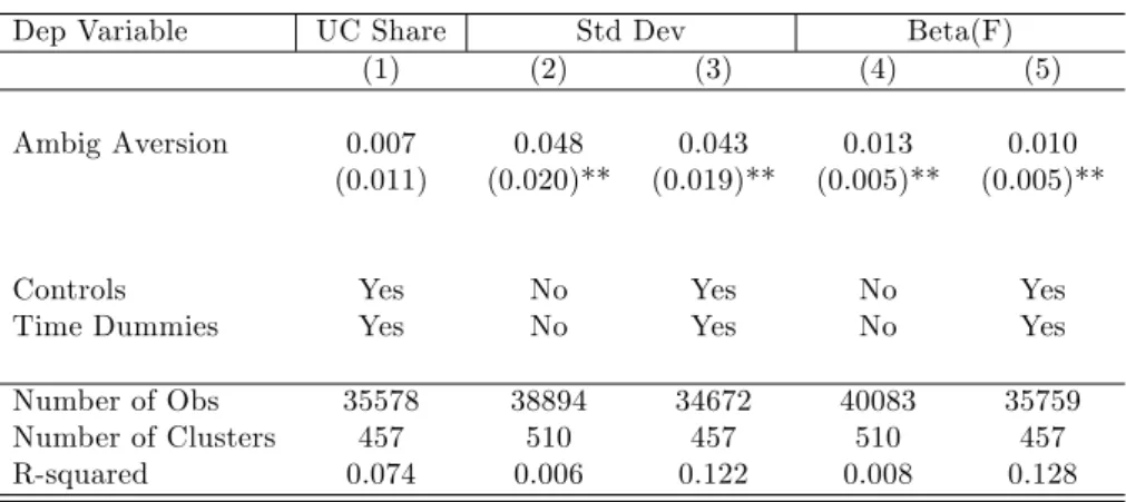
In column 1 of Table 2, the dependent variable is the value of uc funds over the total value of the portfolio at time t. Ambiguity averse investors do not display signi…cantly di¤erent portfolios in terms of composition between euro funds and uc funds. A similar result is obtained by using as dependent variable an indicator of whether the investor holds some uc funds in his portfolio. Hence, we do not …nd evidence that ambiguity aversion leads to non-participation in the stock market through lower investment in uc funds.17 Actually, our …ndings suggest that investors do not view all uc funds as ambiguous.
In columns 2-3, the dependent variable in (1) is the standard deviation of the returns in the previous 12 months (in percentage points). We see that ambiguity averse investors hold more volatile portfolios. A unit increase in Ambiguity Aversion is associated to about 0:04 larger volatility of returns, relative to an average volatility of 0:48. In columns 4-5, the dependent vari-able is Beta(F ), constructed by regressing portfolio returns in the previous 12 months on the French stock market index CAC40. A unit increase in Ambiguity Aversion is associated to about 0:01 larger beta, relative to an average of 0:09.18
The previous results show that more ambiguity averse investors tend to hold portfolios whose returns are more risky, although they do not signif-icantly hold a larger share of uc funds. Following the theoretical insights presented above, we explore whether the extra exposure to risk could be
1 5We asked subjects to report their level of education, age, income and wealth within
pre-speci…ed intervals. In our regressions we include the corresponding ordinal variables. Results would be unchanged if instead we used a series of dummies (see the Online Ap-pendix).
1 6This makes it harder for us to …nd statistically signi…cant results. As shown in the
Online Appendix, standard errors would be much smaller with alternative clustering.
1 7The non-participation hypothesis rests on the prediction of the maxmin expected
utility model that an ambiguity averse investor will not hold an ambiguous asset for a range of prices. Note though that our data set is not ideal to study non-participation as it only captures participation in the stock market through mutual funds.
1 8In the Online Appendix, we show that one gets similar results by constructing these
variables in a forward-looking way based on the standard deviation and beta of the returns in the next 12 months.
driven by a desire to avoid ambiguity.
Taking the theoretical insights to the data is challenging. Ideally, it would require to classify assets in terms of (perceived) ambiguity, for which no general method is available. Some indirect ways have been proposed to estimate ambiguity at the market level.19 At the micro level, the perception may be subjective and hence di¢cult to assess. Moreover, as mentioned, in our data we have no direct information on which individual stocks are included in a given uc fund.
We address the issue in two ways, taking advantage of the fact that we observe realized returns in our data. First, we distinguish portfolios ac-cording to their exposure to the French relative to the international market. Second, similarly to Calvet et al. (2007), we employ standard market fac-tors models in order to estimate the level of idiosyncratic volatility borne by each client. In both cases, the premise is that, while reducing expo-sure to stocks perceived as more ambiguous, ambiguity aversion may lead to portfolio under-diversi…cation.
We start by considering the exposure to foreign stock markets. We com-pute Beta(W ) by regressing portfolio returns in the previous 12 months on the MSCI World Index. In column 1 of Table 3, we observe no signi…cant relation between Beta(W ) and Ambig Aversion. Given the earlier evidence of higher exposure to the French stock market, we are lead to investigate whether ambiguity aversion is associated to a di¤erential exposure to the domestic vs. foreign markets. If we follow conventional wisdom and the above mentioned literature, a higher exposure to international markets is tantamount to bearing higher ambiguity.
The measure we take is simply the di¤erence between Beta(F) and Beta(W). In column 2, we indeed observe that the larger ambiguity aversion the larger is the di¤erence Beta(F)-Beta(W). In column 3, we include the sum of the two betas in order to control for scale e¤ects. The e¤ect of am-biguity aversion is positive and signi…cant, suggesting that amam-biguity averse investors are more exposed to the French rather than to the international stock market. The estimated coe¢cient implies that a standard deviation increase in ambiguity aversion increases the di¤erence Beta(F)-Beta(W) by 0:7%, relative to the average di¤erence of 2:3%.
This is direct evidence that ambiguity aversion is a plausible explanation of the observed home bias in the stock market: portfolios of more ambiguity averse investors are more exposed to domestic stocks than to foreign stocks compared with less ambiguity averse investors.
In a similar vein, Dimmock, Kouwenberg, Mitchell and Peijnenburg (2016) employ a survey question on whether the respondent holds foreign
1 9Antoniou, Harris and Zhang (2015) identify ambiguity with more widespread experts’
forecasts. Jurado, Ludvigson and Ng (2015) assimilate ambiguity with the unpredictable part of the times series studied.
stocks and document a negative relation between foreign stock holding and ambiguity aversion. Our results complement their …ndings. First, we doc-ument home bias starting from information about portfolio returns, as op-posed to self-reported measures of stock holding, which allows to show the consistency between the two approaches. Moreover, our results point at a form of home bias in mutual fund (as opposed to direct stock) holdings, which we …nd particularly remarkable given that mutual funds are com-monly perceived as instruments to obtain well diversi…ed portfolios. Third, as we show in Section 5, we can explore in further details the implications of home bias for realized returns.
We further address the relation between portfolio composition and ambi-guity preferences by investigating to what extent the returns of the portfolios held by our investors are explained by standard market factors. We run the following time-series regressions separately for each client:
ri;t= i+ iCACt+ "i;t; (2)
in which ri;t are the returns experienced by client i at time t, CACt are the
returns of the CAC40 index in percentage points. We then repeat a similar exercise using instead the Fama-French 5 factors model. For each client, we consider the following model:
ri;t = i+ imktrft+ sismbt+ hihmlt+ rirmwt+ cicmat+ i;t; (3)
in which the returns experienced by client i at time t are regressed on the standard 5 Fama-French Global factors.20
For each regression in (2) and in (3), we use the sum of squared residuals (rssi) as a measure of how much the returns of a given portfolio are explained
by its exposure to the market factors and so of how much idiosyncratic risk the agent bears. We also consider the R-squared from these regressions, which indicates the level of idiosyncratic risk relative to total risk. The latter is measured by the variance of the returns, which as showed earlier, tends to increase with ambiguity aversion.
We investigate the relation between idiosyncratic risk and ambiguity preferences in the following regression:
rssi= a + bAmbigAversi+ X
0
ic + "i;
2 0The factors are taken from Kenneth French’s webpage and are explained in Fama
and French (2015). Mktrf denotes the excess return of the market portfolio; smb denotes Small Minus Big; hml denotes High Minus Low; rmw denotes Robust Minus Weak and cma denotes Conservative Minus Aggressive. Our result are qualitatively unchanged when including only some of these factors as well as when including other factors (such as momentum). Similarly, results do not change by considering factors at the European level (whenever available).
in which rssi is the above constructed sum of squared residuals and X
0
i
includes our usual set of controls. In alternative speci…cations, we use the R-squared as dependent variable.
We report our results in Table 3. In column 4, we report a positive relation between ambiguity aversion and rssi as derived in regressions (2).
The same relation is obtained when estimating the sum of squared residuals from the richer model (3), as reported in column 5. Similarly, we observe a negative relation between ambiguity aversion and the R-squared obtained in regressions (3). These estimates show a robust pattern: the higher ambi-guity aversion the lower is the ability of standard market factors to explain portfolio returns. These results suggest that ambiguity averse investors bear more idiosyncratic volatility, also pointing to under-diversi…cation.
5
Portfolio Returns
We now turn to the relation between ambiguity preferences and the re-turns which investors experience in their portfolio. The following regressions should not be viewed as a test of a particular asset pricing model nor as an assessment of the performance of our investors. This would require a well-de…ned normative benchmark about which portfolio our investors should hold, as a function of their characteristics and, in particular the ambigu-ity they perceive. The theoretical literature however does not provide a synthetic benchmark against which one should assess how ambiguity averse investors perform.21 Moreover, as discussed above, we have no direct mea-sure of the ambiguity perceived by investors.
Yet, we do observe the returns of their portfolio and can assess whether, in our sample, more ambiguity averse agents earn higher or lower returns. This type of analysis is new in the literature and it complements the results presented in the previous section by showing their implications in terms of portfolio returns. Furthermore, this analysis points out that it is not necessarily the case that ambiguity averse investors experience lower returns, an observation which is relevant for the theoretical literature on the long-run impact of ambiguity aversion on asset prices. This literature typically builds on the idea that ambiguity averse investors earn lower returns (as expected utility agents with biased beliefs would) and then studies their long-run survival based on market selection arguments (see e.g. Condie (2008) and Guerdijkova and Sciubba (2015)). While di¤erent models may have di¤erent predictions on how much investors would a¤ect asset prices depending on their relative wealth in the economy, or on the speed of decline of lower performing investors, our results question the view that ambiguity averse investors must earn lower returns. Irrespective of the speci…c selection
2 1Hara and Honda (2016) show that any given portfolio can be optimal for certain levels
model at hand, these results suggest that the in‡uence of ambiguity averse investors need not disappear, and this can be seen as a further motivation to incorporate them in asset pricing models.
5.1 Results
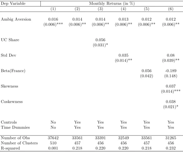
We employ the same speci…cation as in equation (1) and use as dependent variable the monthly returns (in percentage points) experienced by investor i at time t. As benchmark, the average monthly return in the overall sample is 0:38%.
In columns 1 and 2 of Table 4, it appears that in our sample ambigu-ity averse individuals experience higher raw returns. We then add various measures of portfolio risk as controls. In column 3, we include the value of uc funds over the total value of the portfolio; in column 4, the standard deviation of the returns; in column 5, we control for the beta of the returns relative to the French stock market. In column 6, we account for higher moments in the return distribution by including the skewness of the return and the coskewness relative to the French stock market.22 The estimated impact of ambiguity aversion, however, does not change much. Overall, in-vestors with an extra unit of ambiguity aversion experience about 0:012% higher returns per month (that is, about 0:2% per year).
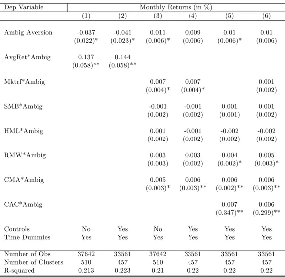
Given the results on portfolio composition documented in the previous section, we then investigate whether these di¤erences in returns are het-erogeneous with respect to market conditions. In Table 5, AvgRet is the average returns (in %) across all portfolios at time t: Our interest is in the interaction with ambiguity preferences. It appears that the higher ambigu-ity aversion, the higher are returns in good times and the lower are returns in bad times. In particular, when average market returns increase by 1%, investors experience 0:14% higher returns for each extra unit of ambiguity aversion. Conversely, ambiguity averse investors experience lower returns when market returns are low.23 These results are consistent with the above
evidence that ambiguity averse investors take more risk, in particular in terms of exposure to the French market. Overall, their returns are higher, but at the same time they are more sensitive to market trends. As in the model by Boyle et al. (2012), under-diversi…cation leads to more volatile returns.
We explore these patterns further by replacing AvgRet with the …ve Fama-French factors introduced in equation (3). We are interested in
inves-2 inves-2We measure the skewness as E[(R R)
3= 3
R], where R and R are respectively
the mean and the standard deviation of the returns R in the previous 12 months. We measure the coskewness as E[(R R)
2(C C)=
2
R C]; where Cand Care respectively
the mean and the standard deviation of the French stock market index CAC40 C in the previous 12 months.
2 3These interactions are not a¤ected when controlling for measures of riskiness of the
tigating whether the returns experienced by investor i at time t depend on the interaction between investor i’s attitude towards ambiguity and a given factor ft. These interactions terms indicate whether more ambiguity averse
investors hold a di¤erent exposure to factor ft.
In columns 3-4, we observe that the larger ambiguity aversion, the larger is the exposure to factor Mktrf, that is the excess return of the market portfolio. Consistently with the previous evidence, a larger exposure to Mktrf would predict higher returns in good times and lower returns in bad times.
As we have shown that ambiguity averse investors tend to be more ex-posed to the French stock market, we then replace Mktrf with CAC, which measures the returns of the French CAC40 Index. In column 5, we observe that ambiguity averse investors have a larger exposure to CAC. When we include both Mktrf and CAC (column 6), we observe that the interaction between ambiguity aversion and Mktrf is no longer signi…cant once the ex-posure to CAC is accounted for. These results are in line with our previous evidence that ambiguity averse investors are overly exposed to the domestic vs. the international stock market.24
Columns 3-6 also show that ambiguity averse investors hold portfolios which are more exposed to "conservative" relative to "aggressive" …rms. This may indicate that aggressive …rms, which display higher rates of in-vestment and growth, are perceived as more ambiguous than conservative …rms (see Fama and French (2015)). Under this assumption, our result is in line with the experimental literature (such as Bossaerts et al. (2010) and Kocher and Trautmann (2013)) showing that ambiguity averse investors are less likely to invest in ambiguous assets. While these authors focus on the implications for the value premium (which would correspond to the HML factor in our regressions), we highlight the interaction with the CMA factor. To our knowledge, this result is new in the literature and we view it as a suggestive line for future research.
6
Portfolio Dynamics
We now turn to investigating whether, depending on their attitudes towards ambiguity, investors display di¤erent portfolio dynamics. A distinctive fea-ture of our database is its panel dimension: we observe clients’ behavior at a monthly frequency for about 9 years. This allows us to explore how investors adjust their portfolio over time, and so to relate to a recent literature on portfolio dynamics under ambiguity aversion.
2 4Notice however that a larger exposure to CAC40 relative to MSCI does not
automat-ically lead to higher returns in our sample period. In this period, the average monthly returns of CAC40 are equal to 0:5% while for MSCI they are equal to 0:7%. We further discuss this point in the Online Appendix, where we show that ambiguity averse investors had higher information ratios in our sample.
6.1 Theoretical Background
Several recent models have shown that ambiguity aversion may lead to forms of portfolio inertia in that households may wish to keep their risk exposure constant over time even upon observing shocks, say, to the distribution of expected returns. Portfolio inertia can have important consequences also for the functioning of asset markets, as it impacts the amount of informa-tion revealed in prices and ultimately their level and volatility (Condie and Ganguli (2012)).
The simplest intuition behind portfolio inertia can be found in a model by Epstein and Schneider (2010) in which any realization of an ambiguous variable entails good news (say about the returns of an asset) and at the same time bad news (say about the variance of these returns). As they show, there exist some portfolio position at which such news o¤set each other and so the agent is completely hedged against ambiguity. This leads to a form of portfolio inertia since it takes a large shock to prices to induce ambiguity averse investors to move away from that position.
The intuition has proven robust in various settings. Illeditsch (2011) considers a more general portfolio choice problem in which agents receive signals of ambiguous precision. He shows that ambiguity averse investors would stick to some intermediate portfolio weights for a range of prices since at these positions agents’ utility becomes independent of the signal precision. Similar results appear in Garlappi et al. (2007) and Ganguli, Condie and Illeditsch (2012), who show that ambiguity averse investors tend to keep their portfolio weights constant as they tend not to respond to news about future returns.
Based on these models, we expect that ambiguity averse investors will be more likely to hold to a given position and therefore rebalance their portfolio to maintain this position over time (i.e. after observing the various returns, that a¤ect the value of the di¤erent funds they hold in their portfolio). Two important observations should be mentioned in relation to our next analysis. First, in the above mentioned models, portfolio inertia occurs even conditional on participation, at positions containing a positive share of ambiguous assets. Second, portfolio inertia does not mean that ambiguity averse investors rebalance their portfolio less frequently. On the contrary, that may require continuous rebalancing so as to compensate the ‡uctuations induced by the market. If, say, realized returns of uc funds exceed those of euro funds, the relative value of uc funds in the portfolio would mechanically increase. If the investor wishes to keep her exposure to uc funds constant, she needs to reallocate wealth from uc funds to euro funds.
6.2 Results
For each investor, we analyze how the value of uc funds over the total value of the portfolio evolves over time. The share of uc funds is only a rough measure of exposure to uncertainty (indeed, we have argued that the composition of uc funds may also matter). At the same time, this measure has the advantage of being simple (it is arguably the most salient characteristic of the portfolio) and of being the closest to the literature. The above mentioned models focus mostly on the fraction of wealth invested in uncertain assets, not on their composition. Our empirical analysis follows closely Calvet et al. (2009), who look at the fraction of wealth invested in uncertain assets, which they call risky share. We adopt the same terminology and, in the next analysis, we refer to the share of uc funds simply as the risky share.
We start by analyzing the intensity of portfolio rebalancing; that is, how much of the observed change in the risky share is driven by active rebalancing as opposed to passive changes induced by past market trends. Denote with Xi;t 1the risky share for individual i at time t 1. If ri;t rf is the realized
excess return of uc funds for individual i between t 1 and t; the passive share is de…ned as
Xi;tP = (1 + ri;t)Xi;t 1 1 + rf+ (ri;t rf)Xi;t 1
: (4)
The change of the risky share from Xi;t 1 to Xi;t; can be decomposed as
follows:
Xi;t = Xi;tP + Xi;tA Xi;tP Xi;t 1 + Xi;t Xi;tP (5)
i.e., it is the sum of the passive change and the active change. We then employ the structural model developed by Calvet et al. (2009) so as to study the intensity of rebalancing by observing the evolution of XP
i;t and
XA
i;t: Calvet et al. (2009) assume that households di¤er in their speed
of adjustment between the passive risky share and an (unobservable) target share, and show that the speed of adjustment can be conveniently estimated under the following conditions. First, the log of the risky share xi;t is a
weighted average between the log of the passive share xPi;t and the log of the (unobservable) target xi;t: Denoting as i the speed of adjustment towards the target share, we have
xi;t= ixi;t+ (1 i)xPi;t+ ui;t: (6)
Second, the speed of adjustment is a linear function of a set of observable household characteristics wi;t; that is,
i = 0+
0
Third, the change in the log target share is a linear function of these char-acteristics,
xi;t = 0;t+
0
twi;t: (8)
An advantage of the log speci…cation is that xi;t can be de…ned indepen-dently of individual-speci…c time-invariant characteristics. Taking the …rst di¤erence of (6), and using i and xi;t from (7) and (8), we obtain
xi;t = at+ b0 xPi;t+ b
0
wi;t xPi;t+ c0twi;t+ w0i;tDtwi;t+ ui;t; (9)
in which at= 0 0;t; b0= 1 0; b = ; ct= 0 t+ 0;tand Dt=
0
t: In
(9), xi;t is the change in the log risky share and xPi;t is the change in the
log passive share where all the changes are expressed in yearly terms (that is, relative to 12 months before). The vector wi;t may include demographic
characteristics as well as portfolio characteristics (returns, standard devia-tion). The coe¢cient b0 measures the fraction of total change in the risky
share which is driven by the passive change. The lower the speed of adjust-ment, the closer b0 should be to 1: Our main interest is in exploring whether
the speed of adjustment varies systematically with ambiguity preferences, which we include in the set of characteristics wi;t:
An important observation in Calvet et al. (2009) is that OLS estimates of b0 and b in equation (9) may be negatively biased since xPi;t and ui;t
may be negatively correlated. From (6) and (9), we can observe that a positive shock to ui;t 1, for example, would reduce ui;t and at the same
time increase xi;t 1; which in turn would increase xPi;t and so increase xPi;t:
An instrument for xPi;t is xIVi;t de…ned as the (log) passive change that would be observed in case the household did not rebalance in period t 1.25 As expected, given partial rebalancing, xIV
i;t is indeed highly correlated
with xP
i;t. The key assumption for the validity of the instrument is that
the returns ri;t are uncorrelated with the error term.
We collect our results in Table 6. In column 1, the OLS estimate of equals 0:37; in column 2, the IV estimate is 0:43: The latter implies that on average our investors rebalance about 57% of their passive change over 12 months. The magnitude is comparable to Calvet et al. (2009), who report estimates around 50% for Swedish households.
In columns 3-5, we investigate whether these e¤ects vary with ambiguity preferences. In column 3, we include no control; in column 4, we include our standard set of controls and time dummies; in column 5, we replicate the full model in (9) by adding portfolio characteristics (returns and standard deviation in the past 12 months), interacting all terms with the passive change (that corresponds to b0wi;t xPi;t) and including the squared terms of
all controls (that corresponds to w0
i;tDtwi;t). These estimates reveal that the
2 5Formally, xIV
i;t = ^xP xPt 1 where ^xP = ln(
(1+ri;t)XPt 1
1+rf+(ri;t rf)XtP1
higher ambiguity aversion the lower is the impact of the passive change on the total change.
In terms of magnitude, each extra unit of ambiguity aversion decreases the e¤ect of the passive change by approximately 26%. According to the estimates in column 4, with Ambiguity Aversion equal to 1, the passive change contributes to the entire change in risk exposure over 12 months. If Ambiguity Aversion is equal to 4, the passive change instead contributes to about 20% of the total change.
These results indicate that ambiguity averse investors display a higher speed of adjustment of their portfolios. As noticed, this may be driven by the desire to keep their risk exposure constant over time, which would be in line with the above mentioned theoretical predictions.
We then look at the direction of rebalancing, described by the sign of the active change relative to the passive change. If active change and pas-sive change have the same sign, for example, the investor is rebalancing his portfolio in the same direction as past market trends: he is increasing his exposure to assets which have performed relatively well in the past. We estimate the following equation:
Xi;tA = + AmbigAversi Xi;tP + Xi;tP + Z
0
i + t+ "i;t: (10)
In equation (10), the coe¢cient estimates the impact of the passive change XP
i;t on the active change Xi;tA.26 If investor i wishes to keep its risk
ex-posure constant over time, he needs to compensate any passive change with an active change of the same magnitude and opposite sign. The coe¢cient should then be close to 1. Our coe¢cients of interest is ; which measures the di¤erential impact of investors’ preferences over ambiguity. The vector Zi0 includes the variables Ambiguity Aversion as well our standard set of controls; t are month-year …xed-e¤ects; standard errors are clustered at
the individual level.
Results appear in Table 7. In column 1, the coe¢cient is 0:63; which implies that on average households compensate about 63% of the passive change in their risky share. This is consistent with the estimates of Table 4 (column 1), and with Calvet et al. (2009), who show that on average households act as rebalancer. Further evidence along those lines is reported in Guiso and Sodini (2013).
In columns 2-5, we observe that the coe¢cient is negative. Estimates are rather stable as we add various controls (column 3), lagged risky share as in Calvet et al. (2009) (column 4) and if we exclude portfolios with zero passive change (column 5). According to these estimates, the larger ambi-guity aversion the closer the estimated impact is to 1. Speci…cally, for the least ambiguity averse investors, a unit increase in the passive change leads
to active change of 0:53. For the most ambiguity averse investors, a unit increase in the passive change leads to an active change of 0:67. Put dif-ferently, for the most ambiguity averse investors, the distance between the risky share and the constant share is on average 1=3 of the passive change. As in our sample the average passive change is 3:8%, that leads to a risky share which is on average 1:3% lower than the constant share.
This evidence is consistent with the theoretical models mentioned above in which ambiguity averse investors may be reluctant to change their expo-sure to uncertainty over time. For this purpose, they need to rebalance their portfolio actively and in a contrarian direction relative to market trends, which is indeed what we observe.
7
Concluding Remarks
Our analysis has provided novel results relating ambiguity preferences to the composition, the returns and the dynamics of household portfolios. We have performed several robustness checks on these results, which we report in details in the Online Appendix. First, we have showed that the e¤ects we observe within the company do not vary systematically with the fraction of wealth invested in the company, suggesting that they are representative of clients’ behaviors in their overall portfolios. We have also checked that some speci…c features of assurance vie contracts, like the possibility of delegated portfolio management and …scal advantages, do not a¤ect our results. On ambiguity aversion, we have considered alternative measures (including pref-erences in the loss domain) as well as their interaction with other behavioral traits (such as sophistication, con…dence, and time preference). Finally, we have discussed our treatment of standard errors and the possibility of sur-vivorship bias in our sample. These tests have shown the robustness of our main …ndings along all these dimensions.
We view this study only as a …rst step towards an understanding of the empirical content of ambiguity preferences in relation to …nancial choices. Further research is needed to assess whether one particular decision model is most relevant to describe investors’ preferences over ambiguity. Our study has identi…ed channels through which ambiguity aversion (measured inde-pendently of a speci…c decision model) a¤ects portfolio behaviors. While this gives some insights on which models are consistent with these e¤ects, it does not provide a direct test of these models.27 Getting richer invest-ment data and …ner measures of ambiguity aversion is an obvious direction of improvement, for which a close collaboration with …nancial institutions is required.
Our results can also be helpful to guide recommendations regarding the
2 7In fact, using a much more structured approach, Ahn et al. (2014) …nd that not one
way individuals’ tolerance for uncertainty should be assessed by …nancial institutions. At the European level for instance, regulation requires …nan-cial institutions to gather information about their clients’ objectives and preferences before selling them …nancial products. What our results sug-gest is that ambiguity aversion should be carefully taken into account when advising individual investors.
References
Ahn, D., Choi, S., Gale, D. and Kariv, S. (2014), ‘Estimating ambigu-ity aversion in a portfolio choice experiment’, Quantitative Economics 5(2), 195–223.
Alvarez, F., Guiso, L. and Lippi, F. (2012), ‘Durable consumption and asset management with transaction and observation costs’, American Eco-nomic Review 102(5), 2272–2300.
Antoniou, C., Harris, R. D. and Zhang, R. (2015), ‘Ambiguity aversion and stock market participation: An empirical analysis’, Journal of Banking & Finance 58, 57 – 70.
Arrondel, L., Borgy, V. and Savignac, F. (2012), ‘L’épargnant au bord de la crise’, Revue d’économie …nancière 108(4), 69–90.
Bauer, R. and Smeets, P. (2015), ‘Social identi…cation and investment deci-sions’, Journal of Economic Behavior and Organization 117, 121–134. Bianchi, M. (2017), ‘Financial literacy and portfolio dynamics’, Journal of
Finance, forthcoming .
Bossaerts, P., Ghirardato, P., Guarnaschelli, S. and Zame, W. R. (2010), ‘Ambiguity in asset markets: Theory and experiment’, Review of Fi-nancial Studies 23(4), 1325–1359.
Boyle, P., Garlappi, L., Uppal, R. and Wang, T. (2012), ‘Keynes meets markowitz: The trade-o¤ between familiarity and diversi…cation’, Man-agement Science 58(2), 253–272.
Butler, J. V., Guiso, L. and Jappelli, T. (2014), ‘The role of intuition and reasoning in driving aversion to risk and ambiguity’, Theory and Deci-sion 77, 455–484.
Caballero, R. J. and Krishnamurthy, A. (2008), ‘Collective risk management in a ‡ight to quality episode’, Journal of Finance 63(5), 2195–2230. Caballero, R. J. and Simsek, A. (2013), ‘Fire sales in a model of complexity’,
Calvet, L. E., Campbell, J. Y. and Sodini, P. (2007), ‘Down or out: Assessing the welfare costs of household investment mistakes’, Journal of Political Economy 115(5), 707–747.
Calvet, L. E., Campbell, J. Y. and Sodini, P. (2009), ‘Fight or ‡ight? portfo-lio rebalancing by individual investors’, Quarterly Journal of Economics 124(1), 301–348.
Campbell, J. Y. (2006), ‘Household …nance’, Journal of Finance 61(4), 1553–1604.
Chew, S. H., Ratchford, M. and Sagi, J. S. (2017), ‘You need to recognize ambiguity to avoid it’, Economic Journal, forthcoming .
Cohen, M., Tallon, J.-M. and Vergnaud, J.-C. (2011), ‘An experimental investigation of imprecision attitude and its relation with risk attitude and impatience’, Theory and Decision 71(1), 81–109.
Collard, F., Mukerji, S., Sheppard, K. and Tallon, J.-M. (2012), ‘Ambiguity and the historical equity premium’.
Condie, S. (2008), ‘Living with ambiguity: prices and survival when in-vestors have heterogeneous preferences for ambiguity’, Economic The-ory 36(1), 81–108.
Condie, S. and Ganguli, J. V. (2012), ‘The pricing e¤ects of ambiguous private information’.
Dimmock, S. G., Kouwenberg, R., Mitchell, O. S. and Peijnenburg, K. (2016), ‘Ambiguity aversion and household portfolio choice puzzles: Empirical evidence’, Journal of Financial Economics 119(3), 559–577. Dimmock, S. G., Kouwenberg, R. and Wakker, P. P. (2016), ‘Ambigu-ity attitudes in a large representative sample’, Management Science 62(5), 1363–1380.
Dorn, D. and Huberman, G. (2005), ‘Talk and action: What individual investors say and what they do’, Review of Finance 9(4), 437–481. Epstein, L. G. and Ji, S. (2013), ‘Ambiguous volatility and asset pricing in
continuous time’, Review of Financial Studies 26(7), 1740–1786. Epstein, L. G. and Miao, J. (2003), ‘A two-person dynamic equilibrium
underambiguity’, Journal of Economic Dynamics & Control 27, 1253– 1288.
Epstein, L. G. and Schneider, M. (2010), ‘Ambiguity and asset markets’, Annual Review of Financial Economics 2(1), 315–346.
Etner, J., Jeleva, M. and Tallon, J.-M. (2012), ‘Decision theory under am-biguity’, Journal of Economic Surveys 26(2), 234–270.
Fama, E. F. and French, K. R. (2015), ‘A …ve-factor asset pricing model’, Journal of Financial Economics 116(1), 1–22.
Fox, C. R. and Tversky, A. (1995), ‘Ambiguity aversion and comparative ignorance’, Quarterly Journal of Economics 110(3), 585–603.
Ganguli, J., Condie, S. and Illeditsch, P. K. (2012), ‘Information inertia’. Garlappi, L., Uppal, R. and Wang, T. (2007), ‘Portfolio selection with
pa-rameter and model uncertainty: A multi-prior approach’, Review of Financial Studies 20(1), 41–81.
Gilboa, I. and Marinacci, M. (2013), Ambiguity and the bayesian paradigm, in ‘Advances in Economics and Econometrics: Volume 1, Economic Theory: Tenth World Congress’, Vol. 49, Cambridge University Press, pp. 179–242.
Gilboa, I. and Schmeidler, D. (1989), ‘Maxmin expected utility with non-unique prior’, Journal of Mathematical Economics 18(2), 141–153. Gneezy, U., Imas, A. and List, J. (2015), ‘Estimating individual ambiguity
aversion: A simple approach’, NBER Working paper 20982 .
Gollier, C. (2011), ‘Portfolio choices and asset prices: The comparative stat-ics of ambiguity aversion’, Review of Economic Studies 78(4), 1329– 1344.
Guerdijkova, A. and Sciubba, E. (2015), ‘Survival with ambiguity’, Journal of Economic Theory 155, 50–94.
Guidolin, M. and Rinaldi, F. (2013), ‘Ambiguity in asset pricing and portfo-lio choice: a review of the literature’, Theory and Decision 74(2), 183– 217.
Guiso, L., Sapienza, P. and Zingales, L. (2017), ‘Time varying risk aversion’, Journal of Financial Economics –forthcoming .
Guiso, L. and Sodini, P. (2013), Household …nance: An emerging …eld, in M. H. G. Constantinides and R. Stulz, eds, ‘Handbook of the Economics of Finance’, Vol. 2, Elsevier, pp. 1397–1532.
Halevy, Y. (2007), ‘Ellsberg revisited: An experimental study’, Economet-rica 75(2), 503–536.
Halevy, Y. (2008), ‘Strotz meets allais: Diminishing impatience and the certainty e¤ect’, American Economic Review 98(3), 1145–62.
Hansen, L. P. (2014), ‘Nobel lecture: Uncertainty outside and inside eco-nomic models’, Journal of Political Economy 122(5), 945–967.
Hansen, L. P. and Sargent, T. J. (2001), ‘Robust control and model uncer-tainty’, American Economic Review 91, 60–66.
Hara, C. and Honda, T. (2016), ‘Asset demand and ambiguity aversion’. Heath, C. and Tversky, A. (1991), ‘Preference and belief: Ambiguity and
competence in choice under uncertainty’, Journal of Risk and Uncer-tainty 4(1), 5–28.
Hey, J. (2014), ‘My experimental meanderings’, Theory and Decision 77(3), 291–295.
Ho¤mann, A. O., Post, T. and Pennings, J. M. (2013), ‘Individual investor perceptions and behavior during the …nancial crisis’, Journal of Banking & Finance 37(1), 60–74.
Illeditsch, P. K. (2011), ‘Ambiguous information, portfolio inertia, and ex-cess volatility’, Journal of Finance 66(6), 2213–2247.
Ju, N. and Miao, J. (2012), ‘Ambiguity, learning, and asset returns’, Econo-metrica 80(2), 559–591.
Jurado, K., Ludvigson, S. C. and Ng, S. (2015), ‘Measuring uncertainty’, American Economic Review 105(3), 1177–1216.
Klibano¤, P., Marinacci, M. and Mukerji, S. (2005), ‘A smooth model of decision making under ambiguity’, Econometrica 73(6), 1849–1892. Knight, F. H. (1921), ‘Risk, uncertainty and pro…t’, New York: Hart,
Scha¤ner and Marx .
Kocher, M. G. and Trautmann, S. T. (2013), ‘Selection into auctions for risky and ambiguous prospects’, Economic Inquiry 51(1), 882–895. Lin, Q. and Riedel, F. (2014), ‘Optimal consumption and portfolio choice
with ambiguity’, Institute of Mathematical Economics Working Paper No 497 .
Maccheroni, F., Marinacci, M. and Ru¢no, D. (2013), ‘Alpha as ambiguity: Robust mean-variance portfolio analysis’, Econometrica 81(3), 1075– 1113.
Machina, M. and Siniscalchi, M. (2014), Ambiguity and ambiguity aversion, Vol. 1 of Handbook of the Economics of Risk and Uncertainty, Elsevier, pp. 729–807.
Riedl, A. and Smeets, P. (2014), ‘Social preferences and portfolio choice’. Ryan, A., Trumbull, G. and Tufano, P. (2011), ‘A brief postwar history of
us consumer …nance’, Business History Review 85(03), 461–498. Trautmann, S. T. and Van De Kuilen, G. (2015), ‘Ambiguity attitudes’,
Handbook of Judgment and Decision Making pp. 89–116.
Uppal, R. and Wang, T. (2003), ‘Model misspeci…cation and underdiversi…-cation’, Journal of Finance 58(6), 2465–2486.
8
Appendix
8.1 Description of variables
Ambig Aversion
The variable is based on the following questions: "You have two options: (a) win 1000 euros with a completely unknown probability vs. (b) win 1000 euros with 50% chance and zero otherwise. Which one would you choose?" If (a) is chosen, we propose (c) win 1000 euros with a completely unknown probability vs. (d) win 1000 euros with 60% chance and zero otherwise. If (b) is chosen, we propose (e) win 1000 euros with a completely unknown probability vs. (f) win 1000 euros with 40% chance and zero otherwise. We build the variable Ambig Aversion which takes values 1 if (a) and (c) are chosen, 2 if (a) and (d) are chosen, 3 if (b) and (e) are chosen, and 4 if (b) and (f) are chosen.
Education
The variable takes value 1 if no formal education is reported, 2 refers to vocational training, 3 refers to baccalaureat, 4 refers to a 2-years post bac diploma, 5 refers to a 3-years post bac diploma, 6 refers to a 4-years post bac diploma, 7 refers to a 5-years post bac diploma or above.
Age
The variable takes value 1 if the respondent is less than 30 years old, 2 refers to between 30 and 44 years old, 3 refers to between 45 and 64 years old, 4 refers to 65 years or older.
Income
Monthly net revenues of the household (in euros). A value of 1 corre-sponds to less than 1000, 2 indicates between 1000 and 1499, 3 indicates between 1500 and 1999, 4 indicates between 2000 and 2999, 5 indicates be-tween 3000 and 4999, 6 indicates 5000 and 6999, 7 indicates bebe-tween 7000 and 9999, 8 indicates over 10000.
Wealth
Total wealth of the household (in euros). A value of 1 corresponds to less than 8000, 2 indicates between 8000 and 14999, 3 indicates between 15000 and 39999, 4 indicates between 40000 and 79999, 5 indicates between 80000 and 149999, 6 indicates 150000 and 224999, 7 indicates between 225000 and 299999, 8 indicates between 300000 and 449999, 9 indicates between 450000 and 749999, 10 indicates between 750000 and 999999, 11 indicates over 1 million.