Saturation dependence of the streaming potential coefficient

HAL Id: hal-03015990

https://hal.archives-ouvertes.fr/hal-03015990

Submitted on 20 Nov 2020

HAL is a multi-disciplinary open access

archive for the deposit and dissemination of

sci-entific research documents, whether they are

pub-lished or not. The documents may come from

L’archive ouverte pluridisciplinaire HAL, est

destinée au dépôt et à la diffusion de documents

scientifiques de niveau recherche, publiés ou non,

émanant des établissements d’enseignement et de

coefficient

Laurence Jouniaux, Vincent Allègre, Renaud Toussaint, Fabio Zyserman

To cite this version:

Laurence Jouniaux, Vincent Allègre, Renaud Toussaint, Fabio Zyserman. Saturation dependence of

the streaming potential coefficient. Seismoelectric Exploration: Theory, Experiments, and

Applica-tions, Wiley, pp.73-100, 2020, 9781119127376. �10.1002/9781119127383.ch5�. �hal-03015990�

Saturation dependence of the streaming potential coefficient

1

L. Jouniaux1, V. All`egre2∗, R. Toussaint1†, F. Zyserman3,4‡ 2

1_{Universit´e de Strasbourg, CNRS, Institut de Physique du Globe de Strasbourg UMR7516, 5 rue Ren´e Descartes, 67084, Strasbourg, France.}

3

2_{Universit´e de Bordeaux, Institut de M´ecanique et d’Ing´enierie, D´epartement G´enie Civil et Environnemental, CNRS UMR 5295, 33615}

4

Pessac cedex, France.

5

3_{Facultad de Ciencias Astron´omicas y Geof´ısicas, Universidad Nacional de La Plata, Paseo del Bosque s/n, B1900FWA La Plata, Argentina}

6 4_CONICET 7 ∗_{[email protected]} †_{[email protected]} ‡_{[email protected]}

Abstract 8

Observations of streaming potential for unsaturated conditions do not always show the same trend de-9

pending on the hydrodynamic conditions and because of a lake of coherency between the data processing 10

procedures. We combine the data from three studies published in the literature, acquired during non-steady 11

state drainage experiments, and apply the same processing steps. We model the hydrodynamic behaviour of 12

these experiments to confirm that they experienced different flow dynamics. We argue that the raw SP data 13

should not be corrected unless a clear drift of the electrodes stability is observed. The combined hydrody-14

namic behaviour and the streaming potential response show that (a) the observations of one of the exper-15

iment (exp #1) are associated to a limited range of water saturation (0.85-1). The corresponding signals could 16

therefore be fairly modelled assuming no saturation dependence of the SPC whatsoever; (b) the observations 17

of exp #3 led to a SPC that can be larger than its value at saturation; (c) the observations of the exp #2 show 18

a non-monotonous behaviour of the SPC as saturation decreases. The underlying physics of a non-monotonous 19

SPC is related to water/air interfaces as shown by the results of the lattice Boltzmann numerical simulations. 20

The main contribution to the SPC behaviour comes from the charged water/air interfaces and depends on 21

the dynamic state of moving or entrapped bubbles. We finally describe the consequences of such a behaviour 22

on the seismoelectric conversions for unsaturated conditions. 23

1 Introduction 24

Electrokinetics are at the origin of geophysical methods used to investigate the near-surface earth sys-25

tem in terms of fluid transfers. Both seismoelectrics and most of self-potentials observations are interpreted 26

to be induced by a relative motion between the rock matrix and the saturating fluid, converted into an elec-27

tric field and a magnetic field through electrokinetic coupling. 28

Seismoelectrics and electroseismics were developed to investigate hydrogeological reservoirs [Dupuis 29

et al., 2007; Dupuis et al., 2009; Schakel et al., 2012; Warden et al., 2013], specially in arid environments

30

[Valuri et al., 2012], and hydrocarbon reservoirs [Thompson et al., 2005; Hornbostel and Thompson, 2007; 31

Hu et al., 2007; Thompson et al., 2007; Zyserman et al., 2012; Guan et al., 2013; Zyserman et al., 2015].

over numerical, experimental and field studies have also investigated borehole geometries [Hunt and Wor-33

thington, 2000; Hu and Liu, 2002; Dupuis et al., 2009; Wang et al., 2015a] and possible applications for

34

the vadose zone [Zyserman et al., 2017a,b; Monachesi et al., 2017]. The reader can find more details with 35

many references in the large review from Jouniaux and Zyserman [2016]. Some other works studied the 36

seismo-electromagnetic signals that could be induced by earthquakes [Matsushima et al., 2002; Gaffet et al., 37

2003; Guglielmi et al., 2006; Ren et al., 2010; Gao et al., 2013, 2016]. 38

Most of the works were developed considering a single saturating fluid at full saturation. It was only 39

in the few last years that attempts to introduce partial saturation in seismoelectrics/electroseismics have been 40

undertaken [Warden et al., 2013; Zyserman et al., 2015]. Besides of using different known effective media 41

models for the different physical parameters of the seismoelectrics/electroseismic equations, the key model 42

parameter, i.e., the electrokinetic coupling, has been modified to cope with partial saturations following the 43

ideas previously used to extend the streaming potential coefficient (SPC) to handle this situations. 44

Self-potentials rely on electrokinetic coupling and proved to be efficient for characterizing groundwa-45

ter resources and mapping contamination plumes, since those signals are directly sensitive to hydrological 46

fluxes [Fournier, 1989; Titov et al., 2002; Pinettes et al., 2002; Maineult et al., 2004; Jouniaux et al., 2009; 47

Desroches and Butler, 2016] and solute transport [Maineult et al., 2005; Kabir et al., 2015; Giampaolo et al.,

48

2016]. Self-potentials appeared especially useful to estimate fluid flow [Jouniaux et al., 1999; Sailhac et al., 49

2004; Rangarajan et al., 2014], to detect propagating vapor-front during oil-extraction processes [e.g., Saun-50

ders et al., 2008], to detect hydrothermal flows [Mauri et al., 2010; Brothelande et al., 2014; Gonzales et al.,

51

2014], to map advected reacting redox fronts [Maineult et al., 2006a,b], and to provide a tool to evaluate the 52

evolution of the corrosion of metallic casings [Maineult, 2016]. Self-potentials are also often associated with 53

natural hydrothermal circulation [Ishido and Pritchett, 1999; Matsushima et al., 2000; Jouniaux and Ishido, 54

2012; Monetti et al., 2014]. The knowledge of the electrokinetic coupling is therefore significant to the in-55

terpretation of a broad range of geophysical methods. 56

Many experimental studies on streaming potential measurements in porous samples have been pub-57

lished in the past three decades [Wang et al., 2015b; Walker et al., 2014; Luong and Sprik, 2014; Glover et al., 58

2012; Glover and D´ery, 2010; Vinogradov et al., 2010; Jaafar et al., 2009; Aizawa et al., 2008; Guichet et al., 59

2006; Perrier and Froidefond, 2003; Hase et al., 2003; Guichet et al., 2003; Jouniaux et al., 2000; Lorne et al., 60

1999; Pozzi and Jouniaux, 1994; Jouniaux et al., 1994; Ishido and Mizutani, 1981]. 61

A few experimental studies addressed the SP (self-potential) behaviour associated with unsaturated flow. 62

Early observations performed during unsaturated water flow experiments on sand showed that SP amplitudes 63

decrease at smaller water content [Guichet et al., 2003], which was supported by some theoretical models 64

[e.g., Perrier and Morat, 2000; Revil et al., 2007]. Linde et al. [2007] proposed similar SP measurements that 65

were also coherent with the existing model by Revil et al. [2007]. 66

The first SPC measurements performed as a function of continuously decreasing water saturation were 67

reported by All`egre et al. [2010]. The raw SPC curves unexpectedly showed a non-monotonic shape as wa-68

ter content decreases, which could not be described by any existing models at the time. Revil and Linde [2011] 69

argued that unconsistent signal processing as well as experimental issues regarding electrode stability were 70

responsible for All`egre et al. [2010] conclusions, which was demonstrated to be very unlikely [All`egre et al., 71

2011]. All`egre et al. [2012] then supported All`egre et al. [2010] observations with a combined modelling of 72

the hydrodynamic conditions and the electrical potential simulating the same drainage experiments. 73

The influence of electrode stability on unsaturated SP measurements has to be treated carefully and 74

was investigated by Jougnot et al. [2012] who proposed that a drifting correction should be applied to raw 75

SP measurements, especially at low water saturation. Another kind of experimental correction was used by 76

Mboh et al. [2012] to address electrode drifting. All`egre et al. [2014] proposed continuous self-potential

mea-77

surements performed during drainage and imbibition cycles. After demonstrating that electrodes were ex-78

tremely stable over time, especially at very low water saturation, they concluded that none of the existing 79

SPC models could correctly describe their observations. A semi-empirical expression addressing the drainage/imbibition 80

cycles dynamics was used to model the SP measurements. The flow dynamics and the behaviour of water/air 81

interfaces were argued to be of significant influence on the response of unsaturated SP [All`egre et al., 2015]. 82

Few theoretical and numerical studies showed that large values of the SPC can be observed under spe-83

cific conditions regarding the chemistry of the electrolyte and structural properties of the porous medium [e.g., 84

Jackson, 2008, 2010]. Numerical simulations performed by Zhang et al. [2014] suggested that the SPC

ex-85

hibits an hysteresis between drainage and imbibition and that it can vary non-monotonically with saturation. 86

Up to this date, neither existing datasets, nor numerical models are entirely consistent. 87

The current contribution aims to reconcile the experimental SP data from Linde et al. [2007], Mboh 88

et al. [2012] and All`egre et al. [2010] by using the same processing steps. We emphasise that the water/air

89

interfaces have to be included in the modelling process so that it can properly describe the unsaturated SP 90

response. 91

2 State of the art 92

We present in this section the theoretical background of the electrokinetics and particularly of the stream-93

ing potential coefficient. We describe the different theories and models of the streaming potential as a func-94

tion of saturation. Then we show measurements of the streaming potential coefficient as a function of the 95

water-saturation. 96

2.1 Theoretical background 97

The electrokinetic effect is due to fluid flow in porous media because of a particular distribution of ions 98

within the electric double layer, which can induce a streaming electric current when water flows, which is 99

counterbalanced by a conduction current. The general equation coupling the different flows is: 100 Ji= N ∑ j=1 LijXj (1)

which links the forces Xj to the macroscopic fluxes Ji, through transport coupling coefficientsLij [Onsager, 101

1931]. Notice that boldface is used to denote vector quantities. 102

In seismoelectrics the coupling between the hydraulic flow and the electric flow is induced by seis-mic wave propagation, which leads to a relative motion between the fluid and the rock matrix. The theory for the coupled electromagnetics and acoustics of porous media was developed by Pride [1994]. The

trans-port relations (Pride, 1994, Eqs. 250 and 251) are: Je= ˆσ(ω)E + ˆL(ω) ( −∇P + ω2_ρf_u s ) , (2) Jf = ˆL(ω)E + k(ω) η ( −∇P + ω2_ρf_u s ) , (3)

where an e−iωt time dependence has been assumed. The electrical fields and mechanical forces that induce 103

the electric current density Je and the fluid volume flux Jf =−iωwf are, respectively, E and (−∇P + 104

iω2ρfus), where P is the pore-fluid pressure, us and wf are respectively the solid and fluid displacements, 105

E is the electric field, ρf is the pore-fluid density, η the dynamic viscosity of the fluid [Pa s], and ω is the 106

angular frequency. 107

The electrokinetic coupling ˆL(ω) describes the coupling between the seismic and electromagnetic fields and is complex and frequency-dependent [Pride, 1994; Reppert et al., 2001]:

ˆ L(ω) = L0   1 − i_ωω c m 4 ( 1− 2d l Λ )2 1 − i3/2_dl √ ωρf η   2   −1 2 , (4)

where m and Λ are geometrical parameters of the pores (Λ is defined in Johnson et al. [1987] and m is in 108

the range 4–8), dl the Debye length. The electrokinetic coupling is an important parameter: if this coupling 109

is zero, then there is no seismo-electric nor electro-seismic conversion. 110

The electrokinetic coupling is related to the streaming potential coefficient ˆCsas

ˆ

L(ω) = −ˆσ(ω) ˆCs(ω); (5)

with σ the rock conductivity. The frequency-dependence of the streaming potential coefficient

[Jou-niaux and Bordes, 2012] can be measured as the ratio between the electric field induced by an applied

pres-sure gradient, when the electric current density Je is zero as:

ˆ

Cs(ω) =

∆V (ω)

∆P (ω) (6)

This coefficient has been studied on synthetic samples [Packard, 1953; Cooke, 1955; Groves and Sears, 1975; 111

Sears and Groves, 1978; Chandler, 1981; Reppert et al., 2001; Schoemaker et al., 2007, 2008], and recently

112

on sand [Tardif et al., 2011], and on unconsolidated materials [Glover et al., 2012]. However the effect of 113

water-saturation has been studied only on steady-state streaming potential coefficient, which is related to the 114

steady-state electrokinetic coupling. 115

The steady-state electrokinetic coupling is defined as:

L0=−σC0(1− 2 ˜

d

Λ), (7)

where the streaming potential coefficient C0 (or SPC) (V P a−1) is defined when the electric current

den-sity Je

Je =−σ∇V − L0∇P, (8)

is zero. 116

When the surface conductivity can be neglected compared to the fluid conductivity, and assuming a laminar fluid flow and identical hydraulic and electric tortuosity, the streaming coefficient is described by the well-known Helmholtz-Smoluchowski equation [e.g., Dukhin and Derjaguin, 1974]:

C0= ∆V ∆P =− L0 σ = SP C = ϵfζ ησf. (9)

The relevant parameters influencing the SPC are the fluid relative permittivity ϵf, the fluid viscosity 117

η, the fluid conductivity σf and the zeta potential ζ, itself depending on rock, fluid composition, and pH. 118

The effect of these parameters has been modeled using Lattice-Boltzmann simulations within a large range 119

of salinity and compared to measured SPC [Fiorentino et al., 2016]. 120

Depending on the type of rocks the surface conductivity may not be negligible as for clay for exam-ple. Then the streaming potential coefficient can be written as:

C0 =

ϵfζ

η(σf_{+ σ} s)

, (10)

with σsthe surface conductivity (S m−1) which can be inferred from σs= 2Σs/R, with R the hydraulic 121

radius of the rock or the pore radius and Σsthe surface conductance (S) [Rutgers, 1940; Alkafeef and Ala-122

jmi, 2006; Wang and Hu, 2012]. In Fontainebleau sand σsis less than 2×10−4S m−1[Guichet et al., 2003]. 123

For quartz or sandstone typical values of Σsrange from 8.9× 10−9to 4.2× 10−8S [Block and Harris, 124

2006] and 2.5× 10−9S for clays [Revil and Glover, 1998]. The surface conductivity can neither be ne-125

glected in clay layers, nor when the hydraulic radius is of the order of the Debye length. This latter case 126

can be encountered when the fluid is not very conductive, as below 2×10−3S m−1in sandstones [Pozzi 127

and Jouniaux, 1994]. In that case the streaming potential coefficient can be lowered compared to the

ex-128

pected value. Since the hydraulic radius can be indirectly connected to the permeability, the effect of sur-129

face conductivity can explain some observations of permeability-dependence of the streaming potential 130

coefficient [Jouniaux and Pozzi, 1995]. 131

Another way to take into account σswithout knowing the surface conductivity nor the conductance

[Jouniaux et al., 2000], but knowing the rock conductivity σ possibly with a surface component and the formation factor F is:

C0=

ϵfζ

ησeff = ϵfζ

ηF σ. (11)

2.2 Streaming potential coefficient modelling for unsaturated conditions 132

The effect of water-saturation on the SPC is still discussed, both through modelling and through the 133

interpretation of the observations, although the effect of saturation on electrical properties is well known [Archie, 134

1942; Carrara et al., 1999; Tsakiroglou and Fleury, 1999; Zhou et al., 2002; Bekri et al., 2003; Jouniaux et al., 135

2006; Kim et al., 2013]. Most of the models for the SPC can be written as a product between the SPC at full 136

saturation Csat and a function of saturation S(Sw) as 137

C0(Sw) = CsatS(Sw) (12)

Perrier and Morat [2000] were the first to propose that the SPC depends on the relative permeability,

and proposed that SPC depends on the relative permeability kras:

C0(Sw) = Csat

kr(Sw)

Swn

, (13)

with Swthe water saturation, and n the second Archie exponent [Archie, 1942], where kr is the relative per-138

meability defined as: kr(Sw) = (Sw− 0.1/0.9)2_{. Later Revil et al. [2007] proposed a similar formula as} 139

proposed by Perrier and Morat [2000], assuming that the excess countercharge density scales inversely with 140

water saturation. 141

Then Jackson [2010] developed a model for the SPC for unsaturated conditions through a capillary tubes model, including water or oil as fluid. Jackson [2010] showed that the electrokinetic coefficient de-pends on the relative permeability, the relative charge density, and the fluid content, assuming that Archie’s law is valid, as:

C0(Sw) = Csat

kr(Sw)Qr(Sw)

Swn

, (14)

with Qr the relative excess charge density: Qr(Sw) = Q(Sw)/Q(Sw= 1). Jackson [2008, 2010] showed 142

that the relative excess charge density depends on the pore-scale distribution of fluid and charge, and that 143

it does not scale inversely with the water saturation. Jackson [2010] showed that the relative excess coun-144

tercharge density increases with decreasing water saturation in water-wet models, because water is first emp-145

tied from the large capillaries. As a result, the water progressively occupies a larger amount of small cap-146

illaries. All these models describe a monotonous decrease of the SPC from Csatto zero with decreasing sat-147

uration, but it has been shown that the relative SPC Cr(i.e., normalized to Csat) could be higher than 1, 148

taking into account the specific flow and electrolyte properties [Jackson, 2010]. 149

All`egre et al. [2012] modelled both Richards’ equation for hydrodynamics and the Poisson’s equation

for electrical potential for unsaturated conditions using a 1-D finite element method, which was never re-ported for unsaturated conditions. They concluded, based on laboratory experiments and using these equa-tions, that the unsaturated electrokinetic coefficient should have a non-monotonic behaviour:

C0= CsatSe[1 + β(1− Se)γ] , (15) where the effective saturation is:

Se=

Sw− Swr 1− Swr

, (16)

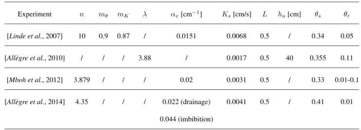
and β and γ are two adjusted parameters, β depending on the initial flow conditions, particularly on the wa-150

ter velocity at the beginning of the drainage phase. Table 1 summarises the values of C0(Sw)/Csat= S(w) 151

gathered from the literature. 152

2.3 Streaming potential coefficient observations for unsaturated conditions 153

The first experimental study on SP dependence on water content was carried out by Guichet et al (2003). They measured the SP associated to water flow during an experiment performed by injecting inert gas into a column filled with Fontainebleau sand (>99% quartz rich sand). The results, corrected from pH and elec-trical conductivity variations (Fig.1), suggested a monotonous and linear behaviour of the SPC as a func-tion of the water saturafunc-tion. They therefore proposed a linear relafunc-tion, via:

C0(Se) = CsatSe. (17)

Linde et al. [2007] measured SP signals associated to a gravity-driven drainage experiment and reported

pres-154

sure head and outflow measurements. They concluded that the SP recordings could be modelled using the 155

model from Revil et al. [2007]. We further discuss the results from this study in section 3. All`egre et al. [2010] 156

reported the first continuous recordings of SP measured during a drainage experiment. Two main important 157

observations were presented: 1) the SPC can be one order of magnitude larger than its value at saturation 158

(Csat); 2) its behaviour can be non-monotonic (first increasing then decreasing) with decreasing water sat-159

uration (Fig.2). The SPC reaches a maximum value that depends on the water flow velocity. No existing mod-160

els could support the dataset. The non-monotonic behaviour of the SPC is partly supported by the observa-161

tions from Revil et al. [2007] and Revil and Cerepi [2004] as discussed in All`egre et al. [2011], once the SPC 162

value measured at saturation from Revil and Cerepi [2004] is properly included (Fig. 3). 163

Vinogradov and Jackson [2011] published SP data acquired during multiphase flow (e.g., water/air or

164

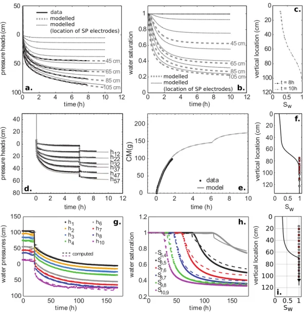
water/oil) imbibition and drainage experiments. They used brine/undecane and brine/nitrogen mixtures. The 165

SP measurements were provided at isolated water saturation values ranging from 0.2 to 0.5. One measure-166

ment was provided for saturated conditions (Fig. 4), but no data points were available for saturation between 167

0.5 and 1. It was therefore difficult to conclude whether the SPC behaviour is non-monotonic in that case. 168

Mboh et al. [2012] reported streaming potential and water pressure measurements performed during

169

a drainage experiment. The authors proposed to remove a trend from the SP data to ensure zero electrical 170

potential difference at the end of the experiment (i.e., in no flow conditions) and the the value. The correc-171

tion also guarantied the SP signal to fit eq. 13 for saturated conditions. The resulting corrected SPC curves 172

were supported by the model from Revil et al. [2007]. This data set is analyzed from scratch in the follow-173

ing section. 174

Jougnot and Linde [2013] performed a few drainage and imbibition experiments providing both SP and

175

hydrodynamic measurements. They observed some features in the SP signals that they attributed to electrode 176

issues. They compared their data set to the one from Mboh et al. [2012] and proposed that SP data should 177

be corrected from electrode effects such as leakage, especially when the medium is quite unsaturated. All`egre 178

et al. [2014] utilized another apparatus to measure self-potentials signals during drainage and imbibition

cy-179

cles. They argued that non-zero SP signals could occur for unsaturated conditions and proposed a water out-180

flow based model to fit their data set. The measurements did not show any evidence for electrode leakage 181

that proved to be extremely stable over time, even for very low saturation values. They suggested that wa-182

ter/air interfaces could be responsible for such variations. The influence of water/air interfaces on SP mea-183

surements is fully discussed in section 4. 184

3 Cross-analysis of streaming-potential data 185

3.1 Background 186

Among the contributions on SP measurements published in the literature, we chose to combine the data 187

from Linde et al. [2007], All`egre et al. [2010] and Mboh et al. [2012], that we refer to as experiments I, II, 188

and III in the following. The three datasets were acquired under similar experimental conditions and exclu-189

sively relate to drainage experiments performed in sand. The raw SP and hydrodynamic data available for 190

each study were used. We included an original dataset acquired using the experimental setup described in 191

All`egre et al. [2014] and designed for drainage/imbibition cycles experiments. We refer to this work as

ex-192

periment IV in the results section. We chose to focus on SP data recorded during non-steady state exper-193

iments, since the dynamics of the water flow is a key parameter. We therefore did not include SPC measure-194

ments performed in consolidated samples in quasi-static conditions [e.g., Revil and Cerepi, 2004; Vinogradov 195

and Jackson, 2011] .

3.2 Experimental procedures 197

The drainage experiment proposed by Linde et al. [2007] was performed in a 135 cm long and 35 mm 198

wide poly-vinyl chloride tube. The medium was a fine grain quartz sand saturated with tap water, whose the 199

electrical conductivity was σw = 0.051 S/m. The bulk electrical conductivity of the saturated mixture was 200

σsat = 0.012 S/m. The water pressure was monitored with ten tensiometers spread along the column (Fig. 201

5). The SP data were measured with 17 non-polarizable electrodes. The water contents were not measured. 202

The experimental course was described as: 1) a drainage phase was triggered by applying a pressure bound-203

ary condition of 9.1 cm high water column at the lower end of the column, while the upper end was open 204

to atmosphere; 2) this lower boundary condition was removed after 6 hours, allowing a free gravity-driven 205

drainage phase to occur. 206

All`egre et al. [2010] experiment consisted in draining a 1.3 m long and 10 cm wide plexiglass column

207

filled with quartzic sand initially saturated with chemically equilibrated water. A constant pressure head of 208

2 cm was applied at the bottom of the column to drive the drainage experiment. The procedure stopped when 209

no outflow was recorded. The water pressure heads, water contents and SP data were monitored at ten lev-210

els inside the column during the experiment (Fig. 5). 211

The experiment by Mboh et al. [2012] was performed in a 217.5 cm long and 5 cm wide plastic tube. 212

The medium was also a quartz sand, compacted on a portion of the column (117.5 cm). The water pressure 213

were measured using 6 tensiometers, and 10 SP electrodes were located along the column (Fig. 5). The pro-214

tocol was designed in three steps: 1) the system was monitored at the hydrodynamic equilibrium (i.e., no 215

flow occurring) for 22 minutes; 2) a Mariotte reservoir was used to apply a constant head at the top for 38 216

minutes; 3) the reservoir is opened allowing a falling head experiment, followed by a drainage phase of the 217

column. 218

The experiment described by All`egre et al. [2014] was designed to monitor self-potential signals as-219

sociated with drainage and imbibition cycles. The authors used a 30 cm long and 10 cm wide plexiglass col-220

umn filled with saturated quartz sand. The singular experiment included here consisted of a step-by-step drainage 221

phase, followed by a step-by-step imbibition phase. The pressure heads and self-potentials were measured 222

at two locations along the column. The procedure consisted in incrementally decreasing the bottom pressure 223

boundary condition to allow drainage. The imbibition phase mimics these steps by incrementally increas-224

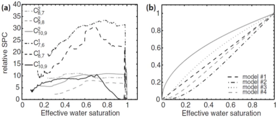
ing the boundary condition until the initial condition was reached. The water contents were computed from 225

solving the flow equation (details in the next section). The SP signals were measured between electrodes lo-226

cated along the column and a reference electrode located at the very bottom, in the saturated part of the sys-227

tem. Using a reference electrode remaining in the water provides a stable potential. This common reference 228

allows to infer any dipole differences afterwards. 229

3.3 Hydrodynamic modelling 230

The hydrodynamic conditions of the experiments need to be constrained so that one can compute the SPC from the computed water pressure differences. Unsaturated flow through a homogeneous porous medium is well described by the Richards equation [Richards, 1931], which is formulated in 1D in its mixed form as, ∂θ(h) ∂t − ∂ ∂z [ K(h) ( ∂h ∂z − 1 )] = 0, (18)

where θ(h) is the volumetric water content in m3_.m−3_{, depending on the pressure head h (m). The} param-231

eter K is the hydraulic conductivity (m.s−1), t is time (s), and z is the vertical coordinate (m), positive down-232

ward. The retention properties and a relative permeability model are necessary to solve eq. 18. Various mod-233

els are available to assess those properties and the studies presented here rely on a few different ones. 234

Linde et al. [2007] used the van Genuchten [1980] model which describes the behaviour of h as a

func-tion of the water content as,

Se=

θ− θr

θs− θr

= 1

(1 + (αv|h|)n₎m, (19)

where Se is the effective water saturation, θsis the water content at saturation, which equals porosity ϕ, θr 235

is the residual water content. The parameter αv (m−1) relates to the air entry pressure, and n and m are two 236

empirical coefficients. 237

Substituting eq. 19 in the capillary model from Mualem [1976] yields to the following relative perme-ability model, K(Se) = KsSeL [ 1− (1 − Se1/m)m ]2 , (20)

with Ksthe hydraulic conductivity at saturation (m/s). The values of m and n are linked by: m = 1−1/n. 238

Usually, this decoupled model is used to improve the results of the parameter optimization of the inverse prob-239

lem [van Genuchten and Nielsen, 1985]. The parameters used in Linde et al. [2007] are reported in Table 3. 240

Associating αv to m and n values in eq. 19 yields to a large air entry pressure. The resulting capillary fringe 241

is almost 40 cm (Fig.6). The capillary fringe is a zone in which water pressure heads can be negative, but 242

which remains saturated (Bear 1972). 243

All`egre et al. [2010] and All`egre et al. [2012] used the model of Brooks and Corey [1964] to address

the retention behaviour of the medium as,

Se = θ− θr θs− θr =        ( ha |h| )λ , if ha_|h| < 1 1 , if ha |h| > 1 (21)

The parameter λ is an estimate of the pore size distribution, characterizing the medium granulometry, the larger the value of λ the more homogeneous the medium. The second hydrodynamic parameter ha is the air entry pressure [Brooks and Corey, 1964] which can be related to αv in eq. (19). The relative permeability behaviour followed the law of Mualem [1976] which leads to,

K(Se) = Ks.SeL+2+ 2

λ, ₍₂₂₎

The parameters used by All`egre et al. [2010] and All`egre et al. [2012] are reported in Table 3. 244

The hydrodynamic measurements from Linde et al. [2007] and All`egre et al. [2010] were modelled us-245

ing the code proposed by All`egre et al. [2012], that solves the electric and hydrodynamic forward problems 246

simultaneously in one dimension. Hydrodynamic behaviour from Mboh et al. [2012] and All`egre et al. [2014] 247

were modelled using Hydrus-1D (www.pc-progress.com), in both cases using the eqs. (19) and (20 ) for re-248

tention and permeability models. The parameter values from the two studies are reported in Table 3. 249

The figures 6a-h show the measured and simulated pressure heads for the experiments I, II and III, as 250

well as the respective vertical profile of saturation inferred from the modelling results. Additional modelling 251

feature include the cumulative outflow measured by Linde et al. [2007], which is a good proxy to check the 252

robustness of the modelling a posteriori. 253

Even though the experimental conditions were similar for all experiments, one can observe that the 254

dynamics varies a lot from one to another. While 10 hours were necessary for experiment I to stop, it took 255

approximately 14 hours for experiment III, and about 200 hours for experiment II. The maximum water flow 256

was therefore much smaller during experiment II. 257

The investigated range of saturation is quite similar as far as the entire column is concerned. However, 258

All`egre et al. [2010] and Mboh et al. [2012] had electrodes located in the part of the medium where the

sat-259

uration significantly decreased (fig. 6c,i) whereas the saturation investigated by Linde et al. [2007] SP mea-260

surements ranged between 0.85 and 1 (Fig. 6f). 261

3.4 Streaming potential measurements 262

During each experiment, streaming potentials were measured between one electrode and a reference 263

located within the saturated part of the column. Additional SP differences can be inferred at any other elec-264

trode locations by subtraction of the raw measurements. The figure 7 compiles the raw SP measurements 265

from experiments I and II. Mboh et al. [2012] corrected raw SP signals using a linear relation designed to 266

address a linear drift between the beginning and the end of the experiment. Following a basic procedure widely 267

reported in the literature [e.g., All`egre et al., 2010; Jougnot and Linde, 2013], we started our analysis back 268

from the raw data and shifted them to zero at the experiment start time (Fig. 7a). Shifting the signals to zero 269

assesses that SP do not exist until water is in motion. Mboh et al. [2012] SP correction also intended to ac-270

count for non-zero electric potential differences at the end of their experiment (i.e., no flow conditions). 271

Jougnot and Linde [2013] analysed Mboh et al. [2012] dataset in combination with one dataset of their

272

own which was acquired during drainage and imbibition experiments. They argued that electrode drifting 273

can be responsible for non-related SP signals, such as non-zero potential differences. Zhang et al. [2014] showed 274

with numerical simulations that non-zero SP could be observed in no flow conditions without the need for 275

the electrodes to be responsible for it. We later argue that the behaviour of water/air interfaces appearing when 276

the medium is unsaturated can be in fact responsible for a priori non-related SP signals. Jougnot and Linde 277

[2013] also wrote that electrode effects were responsible for the behaviour of SP signals observed by All`egre 278

et al. [2010]. All`egre et al. [2015] and Fiorentino et al. [2016] argued that water/air interfaces could be a

plau-279

sible cause for that behaviour. The importance of water/air interfaces is further developed in section 4. Since 280

Jougnot and Linde [2013] demonstrated that the electrodes they used could be unstable over the course of

281

their experiment, we decided not to include their data in this section. 282

SP differences for electrode couples were inferred from raw measurements by subtraction of the raw 283

signals (Fig. 7b-c). The experiment III shows consistently decreasing SP as water saturation decreases (Fig-284

ures 7c), until the dipoles stabilized. The behaviour of SP signals during experiment II is more chaotic with 285

electrodes dipoles showing both decreasing and increasing values when saturation decreases (Fig. 7b). 286

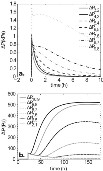
Experiments II and III experienced very different flow dynamics. The figure 8a-b shows the total pres-287

sure differences computed at the location of SP elecrode couples. The recovery of total pressure differences 288

(i.e., pressures differences coming back to equilibrium) which drives the flow, was quite fast in the case of 289

experiment III (Fig.8a). Such a recovery was not reached after 150 hours in the case of experiment II (Fig.8b). 290

The impact of flow dynamics was argued to be of significant effect on the resulting SP response [All`egre 291

et al., 2015].

292

3.5 Streaming-potential modelling 293

The numerical approach of All`egre et al. [2012] allowed us to model the SP responses of experiments 294

I and III. A constant SPC, equal to Csat, and the model from Guichet et al. [2003] (eq. 17) were tested in 295

the procedure. For both studies, the original modelling was performed using the SPC model from Revil et al. 296

[2007]. For experiment I, the hydrodynamic modelling showed that the SP signals were measured within the 297

part of the column that remained saturated during the experiment (Fig. 6f). The modelling results consequently 298

show that the SP signals can be fairly estimated assuming a constant SPC, that equals Csat (Fig. 9). Using 299

the SPC model from Guichet et al. [2003] also leads to a good estimation of SP values. The influence of the 300

SPC model is limited in that case since the saturation remains in the range [0.85; 1], and the electrical po-301

tential is less sensitive to saturation variations. The small SP amplitudes observed by Linde et al. [2007] (|∆V | 302

< 1.1 mV) probably result from the small value of the saturated SPC, Csat=− 7.9×10−7 V.Pa−1. The 303

SP signals measured in the transition zone, where 0.85< Sw <1 (at 25, 35, 60 cm), exhibit a similar

be-304

haviour than the other dipoles located in the saturated part. The experiment I does not show a significant sen-305

sitivity of SP signals to water content variations. Additionally, several models including a constant SPC can 306

fairly predict the measurements. 307

The same approach was used for experiments III (Fig. 10) and experiment IV (Fig. 11). The data from 308

experiment III are not corrected as mentioned in previous section. As for experiment I, the SP are modelled 309

following the approach from All`egre et al. [2012] associated with a constant SPC and Guichet et al. [2003] 310

SPC model. If the trend of SP signals is pretty well described in both cases, the amplitudes of the dipoles 311

from 73 cm to 109 cm are underestimated (Fig. 10). The dipoles from 73 to 109 cm correspond to water 312

saturation ranging from 0.2 to 0.3. The SP measurements from Mboh et al. [2012] are therefore much more 313

sensitive to water saturation than those from experiment I. 314

The experimental SPC curves from experiment III are compared to those from All`egre et al. [2010] ex-315

periment in figure 12. The shape of the SPC from experiment III is significantly altered if no SP correction 316

is applied (Fig. 12a-c). One can notice the significant scattering when the water saturation goes very low, 317

and increasing SPC, which is due to too small pressure difference when using eq. (9). The relative SPC curves 318

from experiment III now exhibit value larger than 1, which is a feature shared with All`egre et al. [2010] re-319

sults. Although the relative SPC can show non-monotonous behaviour for 0.6 < Sw < 0.9 (e.g., Cr/9,8 320

and Cr/7,6 in fig. 12c), it generally decreases when saturation decreases. Interestingly, the relative SPC val-321

ues for experiment II are lower for larger water flow (Fig. 12d), The upper dipole shows higher velocity since 322

the decrease of the water saturation happens for this dipole at the beginning of the drainage. so I would write 323

the reverse which could be be related to the amount and dynamic of water/air interfaces (see next section). 324

Experiment IV was performed with a shorter column (fig.11e), which explains why the drainage phases 325

lasted less than those of experiment III. A few millivolts SP signals was produced overall, which is simi-326

lar to experiment III. Figure 11 presents all of six drainage phases. Although phases d1 and d2 produces a 327

pressure drop and an outflow (Figs. 11a-b), an extremely weak, almost not measurable SP was created. The 328

phases d3 and d4 produced measurable SP drops, that were followed by a recovery phase to zero potential. 329

The following phases are associated to few mV amplitude SP with no recovery. The beginning of phase d5 330

defines a sort of a water saturation threshold beyond which no recovery occurs anymore. Again, the stabi-331

lization of SP signals as soon as the medium is sufficiently unsaturated can easily be related to the influence 332

of water/air interfaces. All`egre et al. [2014] demonstrated that their electrodes were extremely stable during 333

the experiment and not responsible for that stabilization of SP signals. The next section addresses the im-334

portance of the water/air interfaces in the SP response for unsaturated conditions. 335

4 Importance of the interface water/air 336

We saw that the SPC can show a non-monotonous behaviour with the water saturation, and that clas-337

sical models assuming a monotonous behaviour can not be used for unsaturated conditions. For unsaturated 338

conditions two interfaces have to be taken into account: the interface between the matrix and the water, and 339

the interface between the water and the air. Indeed both interfaces are charged and are described as electric 340

double layer or triple layer, and can contribute to the streaming potential through the electrokinetic coupling. 341

Depending on the quantity, mobility, and evolution of these interfaces, according to different conditions of 342

fluid flow such as drainage or imbibition, these contributions can show different behaviours. We describe be-343

low these interfaces, and show some recent results of the modelling of both interfaces using the Lattice Boltz-344

mann approach. 345

4.1 Rock/water interface 346

The interface between rock and water is related to the existence of an electrical double layer between 347

the rock and the fluid. Minerals forming the rock develop an electric double-layer when in contact with an 348

electrolyte, usually resulting from a negatively charged mineral surface. An electric field is created perpen-349

dicular to the surface of the mineral which attracts counterions (usually cations) and repulses anions in the 350

vicinity of the pore matrix interface. The electric double layer (Fig. 13) is made up of the Stern layer, where 351

cations are adsorbed on the surface, and the Gouy diffuse layer, where the number of counterions exceeds 352

the number of anions [Adamson, 1976; Davis et al., 1978; Hunter, 1981]. 353

The distribution of the electrical potential ϕ within the electrical double layer, perpendicular to the solid surface can be calculated resolving the Poisson’s equation:

∇2_{ϕ =−}ρ

ϵf

(23)

where ϵf is the dielectric constant of the fluid. The fluid contains Mi ionic species with valence zi (i=1,...Mi) and number density Nib (the number of species-i ions per unit volume) in the bulk solution far from any charged surface. The charge density ρ can be expressed using a Boltzmann distribution for the ionic species within the fluid: ρ = M ∑ i=1 eziNibexp(− eziϕ kT ) (24)

where k is the Boltzmann constant, -e is the charge of an electron, T is the temperature. It is often as-sumed that the Poisson-Boltzmann equation governing the equilibrium charge clouds can be linearized. As-suming eϕ/kT << 1, the Poisson’s equation becomes:

∇2_{ϕ = (d}l₎−2_ϕ

(25)

with dl _{the Debye length, which is a measure of the thickness of the double diffuse layer, typically} of the order of a few nm:

1 (dl₎2 = M ∑ i=1 e2_z2 iNib ϵfkT (26)

The electrical potential ϕ at a distance x from a charged surface is therefore

ϕ(x) = ζexp(−x

dl) (27)

and ζ is called the zeta potential and is the electrical potential at the shear plane (for further details see Pride 354

[1994]). The zeta potential itself depends on rock, fluid composition, and pH [Ishido and Mizutani, 1981; 355

Jouniaux et al., 1994, 2000; Jouniaux and Pozzi, 1995; Lorne et al., 1999; Guichet et al., 2006; Maineult et al.,

356

2006b; Jaafar et al., 2009; Vinogradov et al., 2010]. 357

The charge density at the surface of the minerals results from surface complexation reactions. The quartz 358

surface can be modelled with silanol > SiOH group [Davis et al., 1978]. The potential-determining ions 359

OH− and H+_{are adsorbed onto the surface of the mineral and determine the charge density on the inner} 360

plane (see figure 13). Therefore the surface charge depends on the pH. There exists a pH for which the to-361

tal surface charge is zero: this is the point of zero charge and pH is called pHpzc [Davis and Kent, 1990; 362

Sposito, 1989]. The charge is positive for pH < pHpzcand negative for pH > pHpzc. In this case this 363

electrokinetic effect is zero. The pHpzc for quartz is in the range 2 < pHpzc < 4 [Parks, 1965; Lorne

364

et al., 1999]. The calcite surface can be modelled with > CaOH and > CO3H groups. Carbonate ions 365

and Ca2+ _{are the determining-potential ions. The electrokinetic behavior on carbonates is more complicated.} 366

The pHpzcvaries from 7 to 10.8 according to the authors [VanCappellen et al., 1993]. 367

It is possible to model simple interfaces and to calculate zeta potential in simple cases [Guichet et al., 368

2006]. This modeling can be performed assuming the triple-layer-model (TLM) which distinguishes three 369

planes to describe the electric double layer: the inner Helmholtz plane for counter ions directly bound to the 370

mineral (assumed to be chemically adsorbed), the outer Helmholtz plane for weakly bound counter ions (as-371

sumed to be physically adsorbed), and a d-plane associated with the smallest distance between the mineral 372

surface and the counter ions in the diffuse layer. It has been proposed that the slipping plane lies near the 373

distance of closest approach of dissociated ions and that the ζ potential can be calculated as the potential 374

on this plane [Davis and Kent, 1990]. 375

At a given pH the most influencing parameter on the streaming potential coefficient is the fluid con-376

ductivity. It has been proposed that C0 = −1.2 × 10−8(σf)−1 [All`egre et al., 2010], based on data col-377

lected in the literature on sandstones and sands (Fig. 14), which leads to a zeta potential equal to−17 mV 378

assuming Eq. (9) and that zeta potential, dielectric constant, and viscosity do not depend on fluid conduc-379

tivity. These assumptions are not exact, but the value of zeta is needed for numerous modellings which usu-380

ally assume the dielectric constant and viscosity independent of the fluid conductivity. Luong and Sprik [2014] 381

also proposed that the zeta potential is constant over a large range of electrolyte concentration. A recent study, 382

taking into account the viscosity and permittivity relationship with the electrolyte concentration, deduced a 383

constant apparent zeta potential of−21 mV, from the comparison of modelling and experimental data set from 384

the literature [Fiorentino et al., 2016]. Therefore an average value of an apparent zeta−20 mV for the needed 385

input value in modellings is fairly exact, at least for media with no clay nor calcite, and in the fluid conduc-386

tivity range excepting very high values. Another formula is often used [Pride and Morgan, 1991] based on 387

quartz minerals rather than on sands and sandstones, which may be less appropriate for field applications 388

when this formula is used in the models without taking into account the effect of the fluid conductivity 389

on all the parameters leading to biaises values of the streaming potential coefficients.. 390

The streaming current is due to the motion of the diffuse layer induced by a fluid pressure difference 391

along the interface. It has been proposed that the streaming current could be used to deduce the perme-392

ability [Jouniaux, 2011; Wang et al., 2016].This streaming current is then balanced by the conduction cur-393

rent, leading to the streaming potential which is proportional to the zeta potential (eq.9): the knowledge of 394

the electric double layer of the rock/water interface and its zeta potential is therefore essential. In the same 395

way the knowledge of the water/air interface is essential and is described below. 396

4.2 Water/air interface 397

Recently All`egre et al. [2015] showed that the interface between water and air should also be taken into 398

account, since this interface is negatively charged, as the interface between the rock matrix and the water. 399

The interface developed between water and air is negatively charged (Fig. 15), the associated zeta po-400

tential being negative and ranging from−65 mV to −35 mV in distilled water [e.g., Graciaa et al., 1995; 401

Takahashi, 2005]. For a water electrical conductivity of 10−2 S/m (equivalent to NaCl concentration of 10−3 402

mol/l) and for pH=7, the zeta potential ranges from−30 mV to −40 mV [e.g., Yang et al., 2001; Creux et al., 403

2007]. We can note that sand/water interfaces are also negatively charged, the associated zeta potential be-404

ing equal to−20 mV. When relative motion occurs at the shear plane of the air/water interface, this results 405

in a streaming current density identical in sign to the current classically created at water/grain interfaces. On 406

the contrary, if the water/air interfaces are dragged, and there is no relative motion, no additional stream-407

ing current will occur. 408

4.3 Evolution of the water/air interface during a drainage 409

One should consider that the streaming current depends on the amount of charges mobilized during 410

a flow. The excess countercharge density depends on the electrical characteristics of the rock/water interface 411

and it has been shown that the matrix/water interfacial area decreases monotonously with decreasing water-412

saturation (Fig. 16) [Culligan et al., 2006]. 413

However the excess countercharge density should also depend on the water/air interfaces in the case 414

of multi-phase flow (water/air/rock). During a drainage phase the surface-area of the water/air interfaces does 415

not decrease with decreasing water-saturation, but first rises to a maximum, and finally decreases. This be-416

haviour has been observed during drainage experiments (Fig. 17) [Culligan et al., 2004], and has been also 417

modelled [e.g., Reeves and Celia, 1996; Berkowitz and Hansen, 2001]). 418

We argue that the behaviour of the unsaturated SPC is related to the surface-area of the water/air in-419

terfaces, since it displays a non-monotonous behaviour as a function of water saturation. This quantity af-420

fects the cohesion of the material: the larger the surface-area of the interfaces, the larger the cohesive stress 421

of the material. It has been shown that the cohesive stress first increases with decreasing water saturation 422

(capillary regime), then reaches a maximum value (within the funicular regime), and finally decreases with 423

further decreasing saturation [e.g., Mitarai and Nori, 2006] (see Fig. 18). During a drainage experiment of 424

a sand column, the upper dipoles first undergo a capillary phase followed by a funicular phase. The upper-425

most sand may be subject to a pendular regime. 426

However to quantify the relative importance of the contribution of the surface-area of the water/air in-427

terface to the surface-area of the matrix/water interface, we developed a two-phase lattice Boltzmann mod-428

elling, whose first results are described in the following section. 429

4.4 Two-phase modelling of steaming potential 430

The streaming potential coefficient has been modelled solving the Navier-Stokes equation and the Poisson-431

Boltzmann equation, using the lattice Boltzmann method in a 2D capillary channel [Fiorentino et al., 2016]. 432

This method allows to model the electrokinetic coupling at a small scale. The flow of an electrolyte within 433

a channel is simulated, as well as the accumulation of charges at the rock/water and water/air interfaces. Then 434

these results are coupled through the computation of the electric field induced by the water flow, via a sec-435

ond Lattice Boltzmann model solving the Poisson-Boltzmann equation. The macroscopic streaming poten-436

tial coefficient is deduced from averaging the electric field on the entire channel and from the pressure dif-437

ference allowing the fluid flow. The presence of water and air within the channel has been studied through 438

several cases: a- the water and the air flows are parallel; b- the air is entrapped within the pores; c- the air 439

flows through bubbles [Fiorentino et al., 2017]. The zeta potential of both interfaces is set at−20mV . 440

4.4.1 Air flow parallel to the channel

441

The water content is decreased by increasing the air content in the middle of the channel: the inter-442

face water/air is therefore parallel to the interface matrix/water, and the diameter of this air corridor is in-443

creasing while the water saturation is decreasing. In this case the surface area of the water/air interface is 444

continuous and constant whatever is the water saturation, except at full water saturation. The streaming po-445

tential coefficient is calculated as a function of the water saturation: C_EKall involves all the sites of the chan-446

nel, C_EKw involves the sites within the water excluding the sites within the air which is not a conducting phase. 447

The streaming potential coefficient is increasing with increasing water saturation, up to the full water sat-448

uration for which the interface water/air does not exist anymore, leading to a decrease of the streaming po-449

tential coefficient (Fig.19). These results show a non monotonous behaviour of the streaming potential co-450

efficient with the water saturation, without involving an increase of the surface area of the water/air inter-451

face. The increase of the SPC with increasing saturation is linked to the increase of the fluid velocity at the 452

interface water/air which is moving towards the centre of the channel when the water saturation is increas-453

ing. Therefore the positive charge excess of the water/air interface is enhanced by a larger velocity, leading 454

to an increase of the SPC. 455

4.4.2 Flow with entrapped bubbles

456

Air bubbles are entrapped on the wall of the channel, with an increasing size for a decreasing water 457

saturation. The resulting SPC is also non monotonous with the water saturation with a possible increase within 458

the range 95% to 80% water saturation (Fig.20). In this case the fluid velocity is decreasing with decreas-459

ing water saturation, and the charge density and the surface area of the water/air interface is increasing, re-460

sulting in such a behaviour of the SPC. 461

4.4.3 Flowing bubbles

462

Air injection in the channel is simulated by flowing an increasing number of bubbles in the centre of 463

the channel, that finally merge together. The streaming potential coefficient shows a non monotonous behaviour 464

with water saturation, linked to a decrease of the fluid velocity with decreasing water saturation, and to an 465

increasing charge density and surface area of the water/air interface with decreasing water saturation (Fig.21). 466

The step in SPC between 55% and 50% is linked to the fact that two bubbles merge into one bubble. The 467

value of the SPC at 82% (star) corresponds to a configuration with more than two bubbles and shows a higher 468

value compared to the SPC value at 82% with two bubbles. The SPC values (dots) involve a zeta potential 469

of−20mV for both matrix/water and water/air interface, whereas the SPC values (crosses) are calculated 470

with a null zeta potential at the interface water/air. The results are therefore very different when the inter-471

face water/air is not taken into account. The non monotonous behaviour of the SPC can hardly be seen when 472

the water/air interface is neglected: the main contribution to the SPC comes from the water/air interface. 473

Therefore these numerical results show that the water/air interface is the main contribution in the elec-474

trokinetic signal for unsaturated conditions, even if the surface area of this interface is constant. An increase 475

of this interface further contribute to the electrokinetic signal. It has to be noted that we made the assump-476

tion that the negative charges causing the zeta potential at the interface air/water are placed in the air phase 477

and stay in the air. They do not contribute to the calculation of the SPC. If these negative charges were in 478

the water, they would contribute to the local electric charge density. In the case of flowing bubbles these charges 479

would move and induce an electric current balancing the electric current due to the excess positive charges. 480

Then the enhancement of the SPC with decreasing saturation would be linked to the difference of velocity 481

between air and water which is near zero. Therefore for flowing bubbles the SPC would not be increased 482

with decreasing saturation, whereas for fixed bubbled the SPC would still first increase with decreasing sat-483

uration and then decrease with further decreasing saturation. We discuss in the following section the effect 484

of different behaviour of the streaming potential coefficient on seismoelectric conversions for unsaturated 485

conditions. 486

5 Consequences on seismoelectric conversions for nonsaturated cases 487

We now describe how the behaviour of the streaming potential coefficient for unsaturated conditions 488

is taken into account in the modelling of the seismoelectric conversions. Then we summarize the seismo-489

electric observations for unsaturated conditions. 490

5.1 Seismoelectric modelling for unsaturated conditions 491

An extension of Pride’s equations aiming to take into account unsaturated materials, in the case of a 492

water-air mixture has been developed by Warden et al. [2013]. The effective medium theory is used to ex-493

press mechanical properties such as the bulk and shear moduli and dynamic viscosity (see Table 2). The medium’s 494

permittivity is derived using the Complex Refractive Index Method, while its conductivity is obtained by ex-495

tending the conductivity derived by Pride [1994] (Equation 242) to partial saturation conditions; this expres-496

sion takes the surface conductivities into account. This approach is combined with the strategy introduced 497

by Strahser et al. [2011], thus writing the dynamic seismoelectric coupling under partial saturation condi-498

tions as a function of the saturation-dependent Streaming Potential Coefficient (SPC). 499

In order to express the static seismoelectric couplingL0 under partial saturation conditions, the SPC 500

at full saturation in Equation 7 is replaced by the saturation-dependent SPC given in Equation 12. One also 501

needs to replace the rock effective conductivity at full saturation in Equation 7 with a saturation-dependent 502

effective conductivity. Using Archie’s second law, that is, neglecting surface conductivities: 503 σ = σ f F S n w= σ f_ϕm_Sn w= σ f ϕ α_∞S n w (28)

Therefore,L0(Sw) can be written as: 504 L0(Sw) =− 1 F ϵfζ η (1− 2 ˜ d Λ)S n wS(Sw) (29)

with Sw a function of saturation being possibly different (see Table 1). 505

By implementing this approach in the GMRT method by Garambois and Dietrich [2002], Warden et al. 506

[2013] studied the interface responses (IR) created by a saturation contrast, and evaluated the influence of 507

the presence of a capillary fringe. They concluded that an IR created by a saturation contrast between sand 508

and sandstone may be easier to detect than a seismoelectric conversion occurring at the same boundary be-509

tween sand and sandstone with the two units fully saturated. Moreover, they proved that the conversions de-510

pend on the type of saturation transition existing between the partially saturated and fully saturated units, 511

as it is depicted in Fig. 22. The extension for the electrokinetic coefficient using different S(Sw) to handle 512

partially saturated media was later used to perform computational simulations of the interface responses at 513

different saturations in a CO2geological deposition site [Zyserman et al., 2015], and to analyze the contam-514

ination of a fresh water aquifer by dense non-aqueous liquids [Munch and Zyserman, 2016]. In the former, 515

it was observed that the IR are sensitive to CO2saturations ranging between 10% and 90%, and that the CO2 516

saturation at which the IR maxima are reached depends on the models employed for S(Sw). Moreover, the 517

simulations predict that the IR’s are still sensitive to different CO2 saturations for a sealed CO2 reservoir 518

covered by a clay layer. For the latter, it was observed that the predicted IR’s are sensitive to different con-519

taminants saturation only when the thickness of the contaminated layer is larger than a threshold value de-520

pending on the properties of the non-aqueous fluid and the saturation function S(Sw); in Fig. 23 this situ-521

ation is depicted. 522

Other authors, e.g., Jardani et al. [2010]; Revil and Jardani [2010]; Revil and Mahardika [2013] pro-523

posed a model alternative to Eq.(29) for the electrokinetic coupling at partial saturation; instead of work-524

ing with the zeta potential, they based the coupling on the excess of electrical charge present in the pore wa-525

ter. However, their model also employs a still not validated -to the authors’ knowledge- relationship between 526

the mentioned excess charges and the rock permeability; this point is discussed by Jouniaux and Zyserman 527

[2015], so that this approach should not be used unless the relation between the excess charge density and 528

the permeability is proved. Within this frame, Revil and Mahardika [2013] studied two-phase flow conditions 529

and proposed a numerical application for water flooding of a non-aqueous phase liquid (NAPL, oil) contam-530

inated aquifer where they observed that seismoelectric conversions mostly take place at the NAPL (oil)/water 531

invasion front and could be used to remotely track its position; Sava et al. [2014] proposed a method to im-532

age the soil electrical resistivity between a set of wells, by mapping the interfaces between different forma-533

tions by means of seismoelectrics, and afterwards deriving the electrical resistivity using crosswell electric 534

tomography. They concluded that the proposed methodology could resolve the fine structure of resistivity 535

between the wells. 536

5.2 Seismoelectric observations for unsaturated conditions 537

The effect of moisture on seismoelectrics was studied in laboratory through experiments performed on 538

samples. However it is difficult to deduce a behaviour of the transfer function as a function of the water-saturation, 539

because of different conditions in the laboratory experiments. 540

The seismoelectric (SE) potential was measured to increase with increasing moisture from 1 to 17 % 541

on samples of limestone, sandstone, aleurolites and marl. At moisture in excess of 15 % a slight decrease 542

was observed in some samples. The inflection of this curve was shifted toward higher moisture values in pro-543

portion to the increase in the concentration of the solution [Gaskarov and Parkhomenko, 1974]. A sharp in-544

crease at low water content was observed in other studies, and could then be constant at increasing water 545

content on dolomite, marl and sandstones, or could decrease on tegillate loam, morainic loam, and limestones 546

for a frequency of the seismic source around 25 kHz [Parkhomenko and Tsze-San, 1964; Parkhomenko and 547

Gaskarov, 1971; Ageeva et al., 1999]. However, at low frequencies (400 Hz compared to 25 kHz) no decrease

548

of the SE effect was observed with increasing water saturation. Only Ageeva et al. [1999] performed mea-549

surements at low frequencies (400 Hz), but they normalized the SE signal to the response of the source of 550

the elastic waves (the test transducer, in V), so that the coseismic transfer function (Eq. 30) cannot be de-551

duced. 552

Seismo-electric conversions in the field can be observed at different conditions of water-content. The water content of the soil can be deduced from electrical resistivity survey or georadar survey. Strahser et al. [2011] observed seismo-electric conversions in the field, as a function of water-saturation, and proposed a trans-fer function between the electric field and the acceleration as a function of the water-saturation. These au-thors proposed to modify the transfer function developed by Garambois and Dietrich [2001], in the low fre-quency assumption valid at seismic frequencies, meaning at frequencies lower than the Biot’s frefre-quency

sep-arating viscous and inertial flows. In this case, and assuming the Biot’s moduli C ≪ H, Garambois and

Dietrich [2001] showed that the SE field E is proportional to the grain acceleration for longitudinal fast P waves:

E≃ −L0

σ ρ

f_{u =¨} ϵfζ

ησf ρ

f_{u.¨ (30)}

Based on their field observations Strahser et al. [2011] proposed that in the low frequency domain, taking into account the water saturation, the SE field and the seismic field are related as:

E≃ ϵζ

ησfS

(0.42± 0.25)n

e dfu.¨ (31)

These observations could not be performed in a large range of water-content, leading to relatively scattered 553

data. 554

Recently the effect of water saturation on coseismic SE signals was studied on sand [Bordes et al., 2015]. 555

Experiments were performed during imbibition and drainage for several cycles, and the water-content was 556

measured by capacitance probes. These authors developed as seismic source a steel ball hitting a granite cylin-557

der in contact with the sand [S´en´echal et al., 2010], showing a main frequency content of about 1.5 kHz and 558

inducing direct P wave [Barri`ere et al., 2012]. The electric signal was recorded by electrodes dipoles (10 559

cm apart) along the P wave propagation. The authors estimated the transfer function of the electric field (elec-560

tric field over acceleration) by picking the arrival in time domain, and by a spectral analysis using contin-561

uous wavelet transform. Both methods showed that these ratios are of the order of 2–7×10−4 V m−2 s−2

562

(depending on the offset to the source) and are rather constant in the water saturation range 0.2–0.9 for im-563

bibition and drainage experiments. None of the tested models for the water-saturation dependence of the SPC 564

could model correctly a constant transfer function in this range of saturation. 565

6 Discussion and conclusions 566

Measurements of SP for unsaturated conditions published in the literature do not always show the same 567

trend, because they can depend on the conditions of the experiment. Whether the experiment consists of a 568

drainage phase, of an imbibition phase, or uses air injection, results in very different pressure behaviours (Fig. 569

8), and leads to a different SP response. We show that the raw SP data should not be corrected for a drift 570

if the electrodes are stable in a saturated medium. The apparent drift of the SP signals is due to water/air 571