Generation and Intensification of Mesoscale Anticyclones by Orographic Wind Jets: The Case of Ierapetra Eddies Forced by the Etesians

HAL Id: hal-03027412

https://hal.sorbonne-universite.fr/hal-03027412

HAL is a multi-disciplinary open access archive for the deposit and dissemination of sci-entific research documents, whether they are pub-lished or not. The documents may come from teaching and research institutions in France or abroad, or from public or private research centers.

L’archive ouverte pluridisciplinaire HAL, est destinée au dépôt et à la diffusion de documents scientifiques de niveau recherche, publiés ou non, émanant des établissements d’enseignement et de recherche français ou étrangers, des laboratoires publics ou privés.

Generation and Intensification of Mesoscale

Anticyclones by Orographic Wind Jets: The Case of

Ierapetra Eddies Forced by the Etesians

Artemis Ioannou, Alexandre Stegner, Thomas Dubos, Briac Le Vu, Sabrina

Speich

To cite this version:

Artemis Ioannou, Alexandre Stegner, Thomas Dubos, Briac Le Vu, Sabrina Speich. Generation and Intensification of Mesoscale Anticyclones by Orographic Wind Jets: The Case of Ierapetra Eddies Forced by the Etesians. Journal of Geophysical Research. Oceans, Wiley-Blackwell, 2020, 125 (8), �10.1029/2019JC015810�. �hal-03027412�

Generation and Intensification of Mesoscale Anticyclones by

Orographic Wind Jets: The Case of Ierapetra Eddies forced by the

Etesians

Artemis Ioannou1, Alexandre Stegner1, Thomas Dubos1, Briac Le Vu1and Sabrina Speich2

1_{Laboratoire de Météorologie Dynamique, CNRS, Ecole Polytechnique, Palaiseau, 91128, France}

2_{Laboratoire de Météorologie Dynamique, CNRS, Ecole Normale Supérieure, 24 Rue Lhomond 75005 Paris, France}

Abstract

Motivated by the recurrent formation and intensification of the Ierapetra anticyclones in the south-east of Crete, we investigated with a reduced gravity model the response of the oceanic surface layer to a seasonal wind jet that varies slowly (over several weeks or months) and mimics the Etesian winds. Our study answers why the oceanic response to such forcing is mainly a large and intense anticyclone. We build a dimensionless parameter that integrates in time the Ekman pumping and quantifies the rel-ative amplitude of the isopycnal displacement induced by the local wind stress curl. According to the range of the wind forcing parameter, the oceanic response to a symmetric wind jet could be a symmetric dipole or a strongly asymmetric structure dominated by an intense and robust anticyclone. This intrinsic asymmetry is driven by the finite isopycnal displacements that occur when the wind forcing parameter reaches unity. Since, the anticyclonic wind shear, for the Etesian wind jet, is two times larger than the cy-clonic one, the asymmetry of the oceanic response is enhanced. Several weeks after the wind forcing has stopped, an intense mesoscale anticyclone which satisfies the cyclogeostrophic balance remains. More-over, if a similar wind jet blows on a pre-existing anticyclone, the latter remains robust and coherent and gets re-intensified in agreement with the previous analysis of remote sensing observations. Hence, this paper is the first numerical study which provides a dynamical understanding for the formation of the single Ierapetra anticyclones and explains their intensification one year after formation.

Corresponding Author: Artemis Ioannou, innartemis@gmail.com Doi: 10.1029/2019JC015810

1 Introduction

The prevailing wind regime over the Eastern Mediterranean Sea (EMS) is dominated by persistent northern winds called Etesians. Every summer, numerous islands in the Aegean are subject to the Etesian wind forc-ing which results in strong upwellforc-ing regions along the east part of the Aegean (Bakun and Agostini,2001). The complex topography of the islands acts as an obstacle for wind propagation inducing channeling and deflection effects towards the south Aegean and the Levantine basin. Kotroni et al.(2001) were the first to demonstrate the blocking and the deflection of the Etesians by Crete island. Performing simulations with and without Crete, they concluded that the Crete orography (3 mountains in the row with height around 2000 m) creates a blocking effect resulting in a deceleration region upstream of the mountains which mod-ifies the Etesian intensity and pathways. Miglietta et al.(2013) simulated the influence of the orography in the south east of Crete, capturing the lee waves patterns in the wakes of the Crete, Karpathos, Kasos and Rhodes islands. Based on observational data from meteorological stations,Koletsis et al.(2009,2010) con-firmed that the Etesians decelerate upstream of Crete and deflect leftward while intensifying between the mountain gaps. Velocities of the maximum wind gusts were recorded to reach 25 m s−1_{in 2007 persisting} for 3 days. The Etesians are observed every summer while their duration is intermittent. They are char-acterized by recurrent periods of gale-force northerlies interrupted by quieter spells (Tyrlis and Lelieveld,

2013). Based on Etesian trends and climatology from 1979 to 2009 (Poupkou et al.,2011), the total number of Etesian days from June to September is on average 45 days with wind forcing values that range between 5 − 15m s−1.

Meanwhile, several long lived oceanic eddies are formed downstream of Crete, in the North Levantine basin. For instance, in the south east corner of Crete, the mesoscale Ierapetra anticyclone is recurrently formed during summer. The role of these Ierapetra eddies (IEs) on the circulation of the Levantine basin has been subject of numerous studies (Hamad et al.,2005,2006;Larnicol et al.,1995;Matteoda and Glenn,1996;

Taupier-Letage et al.,2007). More recently, thanks to the efficiency of automatic eddy detection algorithms applied to high-resolution AVISO/DUACS maps (gridded at (1/8)oin the Mediterranean Sea), the seasonal evolution and the inter annual variability of the IE’s were investigated for more than twenty years (Ioannou et al.,2017). The Ierapetra anticyclones were found to be the most intense eddies of the Levantine basin. The Rossby numbers experience a strong seasonal and interannual variability and could vary by a factor 4 from one year to another. Besides, it was found that the geostrophic assumption underestimates the intensity of these anticyclones and therefore the cyclostrophic corrections should be added to the geostrophic surface velocity field derived for altimetry maps (Ioannou et al.,2019). According to these corrections, the core vorticity could reach intense negative values up to −f (the Coriolis parameter). Moreover, we also found that after their formation, IEs could reintensify (Ioannou et al.,2017). This intensification process may lead to a doubling of the eddy intensity in less than 4 months. Both the formation or the intensification stages coincide with the period of strong Etesian winds when the IEs are located in the southeast of Crete in the lee of the Kasos strait.

The pioneering studies ofHorton et al.(1994) andFusco et al.(2003) have suggested that the IEs were wind forced. Moreover, the statistical analysis of the monthly surface wind (averaged over 20 years) performed byMkhinini et al.(2014) confirmed the presence of strong negative wind stress curl in the south east cor-ner of Crete. Such seasonal correlations between the formation area of the Ierapetra anticyclones and the location of this region of negative wind stress curl seems to confirm the hypothesis that IEs are wind in-duced. But, correlation does not imply causation and the main goal of this paper is to investigate if the specific orographic wind jet induced by the Crete orography could indeed explain the generations and the intensifications of strong Ierapetra anticyclones.

Several cases of coastal eddies induced by orographic winds have been previously observed in several re-gions. For instance, the formation of both cyclonic and anticyclonic eddies are frequently observed in the lee of mountainous islands (Barton et al.,2000;Caldeira et al.,2014;Caldeira and Marchesiello,2002;

Caldeira and Sangrá,2012;Couvelard et al.,2012;Jia et al.,2011;Jiménez et al.,2008;Kersalé et al.,2011;

Piedeleu et al.,2009;Yoshida et al.,2010). The role of the local wind stress as a driver of oceanic vortices was first noted byPatzert(1969), in a discussion of the role of Ekman pumping in generating Hawaiian lee eddies.Yoshida et al.(2010) compared the timescale variability of the kinetic energy and sea surface height of the eddies with the wind stress curl variability downstream of the Hawaii archipelago. A lag of 2 weeks be-tween the oceanic and atmospheric response was found, emphasizing that the ocean acts like an integrator of the wind forcing for low frequencies. For the Hawaiian case, the interaction between the North Equa-torial Current and the archipelago is enough to generate eddies, but high resolution wind stress curl was needed in the numerical models to get the correct eddy intensities in agreement with observations (Calil et al.,2008;Jia et al.,2011;Kersalé et al.,2011). For Madeira Island, both numerical simulations ( Couve-lard et al.,2012) and oceanic observations (Caldeira et al.,2014) indicate that the orographic wind wakes could be the main mechanism of oceanic eddy generation. For larger coastal mountain chains, orographic gaps or valleys could locally amplify the upstream synoptic winds and lead to strong wind jets on the sea. The numerical study ofPullen et al.(2008) has shown that intensified wind jets in the lee of Mindoro and Luzon Islands induce the generation and the migration of a pair of counter-rotating oceanic eddies. More recently,Zhai and Bower(2013) investigated the response of the Red Sea to the Tokar wind jet. Remote sensing and in situ observations both showed that an intense dipolar eddy is formed during the summer monsoon season and that its strength is closely correlated with the wind variability. Besides, the dipolar re-sponse of a 1.5-layer shallow water model, forced by an idealized wind jet, showed a correct agreement with the oceanic observations. All these studies exhibit a dipolar response to the wind jet, in other words both cyclonic and anticyclonic eddies are expected to be formed in the coastal ocean. These results seem to con-tradict the hypothesis that the Ierapetra anticyclones are mainly driven by the Etesian winds. Why would the main response of the wind jet in the Kasos strait be only a large and intense anticyclone ? The underlying mechanism responsible for such asymmetry is not clear. The paper ofMcCreary et al.(1989), which studied

the response of the ocean to the gap winds in the Gulf of Tehuantepec, is the only one which exhibits an asymmetric response which favors the formation of a large scale anticyclone. However, they used a specific shallow-water model which includes a parametrization of the entrainment of cool water into the surface layer. Therefore, it is difficult to determine whether the source of this asymmetry is due to the dynamical response of the oceanic layer or to thermodynamic processes.

In order to study the role of Etesian winds on the formation of intense Ierapetra anticyclones, we will use an idealized reduced gravity shallow water model to mimic the various responses of the upper oceanic layer, above the thermocline, to orographic wind jets. This oceanic layer will be forced only by the surface wind stress and the internal mixing or the atmospheric heat fluxes will be not be taken into account. The main objective of this study is to determine whether Etesian winds alone can explain the formation and the inten-sification of IE’s in agreement with our previous analysis of remote sensing data sets (Ioannou et al.,2017). The paper is organized as follows. In section 2, we describe the 1.5-layer rotating shallow water model as well as the eddy detection and tracking algorithm AMEDA that we use to quantify the dynamical properties of the generated eddies. Section 3 presents the spatio-temporal characteristics of the wind jet according to the regional wind climatology. In section 4 we present the characteristics of the oceanic eddies generated by symmetric and asymmetric Etesian wind jets. The impact of the Etesian wind on pre-existing anticyclone is then presented in section 5. Finally, we discuss, in section 6, the asymmetry of the oceanic response to the Etesian wind jets and compare it to the dynamical characteristics of observed IE’s.

2 Data and Methods

2.1 Wind Data

We use the ALADIN atmospheric data-set (Hamon et al.,2016;Tramblay et al.,2013) to analyze the spatial structure of the Etesian wind forcing and their temporal variations. Based on dynamical downscaling of the ERA-Interim reanalysis, the ALADIN datasets provide the wind stress components for the Mediterranean Sea at a grid resolution of (1/12)o with a time interval of 3 hr . Wind forcing data were extracted for the Eastern Part of the Mediterranean from 1993 to 2012. As we are interested in the slow response of the ocean to the wind forcing a 7 day sliding window is applied in order to filter out short-term variations of the forcing. For the region of interest we additionally collected wind and temperature data from the Greek National Meteorological Service from available meteorological stations in the islands of Crete and Karpathos.

2.2 Rotating Shallow-Water Model

In order to study the dynamical response of the oceanic surface layer to a transient wind jet, we use an ide-alized 1.5-layer model. This ideide-alized rotating shallow-water model also called the reduced gravity model, represents the upper oceanic thermocline with a single active layer of densityρ1which overlays a motion-less layer of infinite depth with higher densityρ2. The unperturbed layer thickness H of the upper layer and the reduced gravity g0 = ∆ρ_ρ2g , where g is the gravitational acceleration and∆ρ = (ρ2− ρ1) the den-sity difference between the two layers, are the two key parameters that we prescribe according to the non uniform stratification of the area (Appendix A). We estimate first the baroclinic deformation radius to be Rd = 10 − 13 km (Chelton et al.,1998) while we choose the unperturbed layer thickness H = 100m. The momentum and continuity equations for the 1.5-layer model are

∂u ∂t + u · ∇u + f k × u = −∇φ + g0τ ρφ+ Ah4 2_{u (1)} ∂φ ∂t + ∇ · (φu) = 0 (2)

where u=(u,v) are the Cartesian components of the horizontal velocity in both directions, f is the Coriolis parameter ( f = 10−4), g0= 0.02 ms−2 is the reduced gravity,φ = g0h is the geopotential height with h the

deviation of the layer thickness andτ = (τx,τy) the wind stress vector. A bi-Laplacian dissipation is used in order to filter out small scale numerical noise that may occur at grid scale. We define four dimensionless numbers associated to such transient wind forcing, the Rossby number RoW, the Burger number BuW, the dimensionless wind evolution tW and the equivalent Reynolds ReW number as follows

RoW =_{f W}UE BuW= µ_R d W ¶2 tW = T f ReW = UEW3 Ah where Rd= p g0_H

f is the first baroclinic deformation radius, UE= τo

ρ f H is the Ekman velocity, W the width of the wind jet and Ahthe hyperviscocity coefficient.

When the wind Rossby number is small (RoW ¿ 1) and the wind evolution is slow enough (tWÀ 1), the first two terms of the momentum equationEquation 1are negligible in relation to the Coriolis acceleration and the initial response of the oceanic layer will satisfy the geostrophic balance. Since we consider relatively slow variations of the wind forcing (tW À 1), most of the work induced by the wind stress at the ocean surface will be transfered to the balanced flow while the generation of inertia gravity waves will be strongly reduced. The Burger number compares the wind jet width to the baroclinic deformation radius while the equivalent Reynolds number compares the relative amplitude of the advective terms to the dissipative terms. The hyperviscosity coefficient was fixed to the constant value Ah= 106m4s−1in order to get at the grid scale UE(∆x)3/Ah∼ 1 while ReW À 1.

The rotating shallow water equations are solved with a doubly periodic boundary condition in a square domain of size Lx× Ly= 600 × 600 km. This domain was chosen to be much larger than the wind jet width W . The horizontal resolution is∆x = ∆y = 1km for all simulations in order to be significantly smaller than the radius of deformation Rd= 13 km. Moreover, the convergence of the numerical solution was tested by comparing the results obtained with decreasing grid sizes.

2.3 The AMEDA Eddy Detection and Tracking Algorithm

To track eddies in the computational domain we use the Angular Momentum Eddy Detection and tracking Algorithm (AMEDA) (Le Vu et al.,2018). Applied to the velocity fields AMEDA identifies the eddy character-istics based on the physical parameters and the velocity field geometrical properties. The eddy centers are first identified and correspond to an extrema of the local normalized angular momentum. The streamlines surrounding this center are then computed (Figure 1). The mean radius 〈R〉 and the mean velocity 〈V 〉 are evaluated for each closed streamline. This mean radius 〈R〉 is defined as the equivalent radius of a circular disc with the same area A as the one delimited by the closed streamline (Equation 3), while the mean veloc-ity amplitude 〈V 〉 is derived from the circulation along the closed streamline C , where Lpis the streamline perimeter (Equation 4). 〈R〉 =pA/π (3) 〈V 〉 = 1 Lp ˛ C V d l (4)

We plot inFigure 1c the pair of the mean eddy velocity 〈V 〉 and the mean radius 〈R〉 for each closed stream-line. We can see on this example that the mean velocity increases when the radius increases until a max-imum velocity Vmax is reached. The corresponding radius is named Rmax, also called the speed radius (Chelton et al.(2011);Laxenaire et al.(2018);Le Vu et al.(2018)). The characteristic contour of the detected eddy (black solid contour inFigure 1) is associated with the closed streamline of maximal speed. After this maxima, the azimuthal speed of the eddy decreases until the last closed streamline is reached. The latter is plotted with a black dashed line inFigure 1. From the characteristic eddy velocity Vmax and the corre-sponding radius Rmax, we compute the vortex Rossby number to quantify the eddy intensity and the Burger number to quantify the relative size of the eddy in respect with the deformation radius Rd:

Ro = ¯ ¯ ¯ ¯ Vmax f Rmax ¯ ¯ ¯ ¯ (5) Bu = µ _R d Rmax ¶2 (6) where f is the Coriolis parameter. We also introduce the dimensionless amplitude of the isopycnal deviation induced by the eddy

λ = η

H (7)

whereη = h(r = 0) − H is the deviation of the surface layer in the eddy core and H the thickness of the unperturbed layer.

Moreover to characterize the eddy shape two geometrical parameters were used. The first one is the ellip-ticityε of the characteristic contour. The second one is the steepness parameter α which is used to fit the mean velocity profile 〈V 〉 = F (〈R〉) of quasi-circular eddies (ε < 0.2) with the generic functions:

V_θ(r ) =Vmax Rmax

r e(1−(r /Rmax)α)/α (8)

Such generic profiles were used byCarton et al.(1989);Stegner and Dritschel(2000);Lazar et al.(2013);

Yim et al.(2019) to study the stability of various isolated eddies. According to (Ioannou et al.,2017,2019) quasi-circular eddies detected by the AMEDA algorithm on the AVISO/DUACS products, and especially the Ierapetra eddies, are correctly approximated by this generic velocity profile (Equation 8). The steepness parameterα varies between α = 1.2 and α = 2.7 while the highest probability is close to the Gaussian shape (α = 2).

Figure 1: The first panel (a) shows the characteristic contour (black solid line) and the last contour (black dashed line)

calculated by the AMEDA algorithm for an anticyclone. The background colors correspond to the relative vorticity fields_{ζ/f and the black vectors to the surface velocity components. The central panel (b) shows the streamlines} associated with the velocity field as well as the characteristic (solid dark line) and the last closed contour (black dashed line). The velocity profile 〈V 〉 = F (〈R〉) deduced from the streamlines analysis is plotted in the right panel (c). We use here negative values for the mean velocities 〈V 〉 of anticyclones. The shape parameter isα = 1.9.

3 Characteristics of the Etesian Wind Jets Between Crete and Kasos

3.1 Etesian Wind Forcing Climatology

Figure 2shows the 20 year averaged (1993-2012) wind stress components 〈τ〉 and the wind stress curl 〈∇ × τ〉 obtained from ALADIN data for the winter (a) and the summer months (b). Areas of positive and negative vorticity fields are distinguished downstream of the islands. The strongest negative wind stress curl, which

Figure 2: (a) Climatological wind stress 〈τ〉 (vectors) and wind stress curl 〈∇ × τ〉 (colors) for the winter (a) and summer

(b) months based on ALADIN datasets (1993-2012). The climatological position of the Ierapetra eddy (1993-2014) is shown with the black contour and the position where all Ierapetra eddies were detected with the black points. The selected area for analyzing the wind forcing climatology is illustrated with the blue circle. (b) The mean monthly climatological wind stress 〈τ〉 and wind stress curl 〈∇ × τ〉 variations in 20 years are shown in panels (c) and (d) respec-tively.

is expected to induce a strong downwelling of the isopycnals, is found in summer at the southeast of Crete downstream of Kasos strait. This is a result of the Etesian wind blocking caused by the Crete’s, Kasos and Karpathos orography, that creates funneling effects between the mountain gaps and the straits separating the islands (Kotroni et al.,2001;Zecchetto and Biasio,2007). During the winter months, the negative wind stress curl is less intense and confined to a much smaller areaFigure 2a. The mean climatological position of the Ierapetra anticyclone, derived from 20 years averaged sea surface height, is marked inFigure 2b with a black contour. The first detection of all Ierapetra eddies from 1993-2014 are illustrated with the black dots as found inIoannou et al.(2017). This correlation between the formation of IE’s, its mean location and the area of strong negative wind stress curl was already highlighted byMkhinini et al.(2014). Although, this represents a mean state of the Etesian forcing and does not account for the spatiotemporal variations of this orographic wind jet. Hence, to illustrate the variations of the Etesian forcing near the mean IE position, we select a circled area of radius R = 60km centered at (27.10oE , 34.7oN ) near the maximum wind stress

Figure 2a. Figure 2c and 2d shows the monthly means of the wind stress components 〈τ〉 and the wind stress curl 〈∇ × τ〉 averaged for the 20 years. Even though the wind stress can be relatively high among all seasons (Figure 2c) the strongest negative wind stress curl is observed during the summer months (Figure 2b and 2d).

In order to simplify the problem we will use, asMcCreary et al.(1989) orZhai and Bower(2013), an ide-alized wind jet having roughly the same characteristics as the Etesian wind forcing. We therefore extract the monthly wind stress and wind stress curl components along 4 sections (Figure 3a), one parallel to the mean direction of the wind and 3 other ones, that spans from 26oE to 28oE in three different latitudes (34.8oN , 35oN , 35.2oN ), cross to the mean climatological wind forcing during the same period. The shape of the mean normalized wind forcing is shown for the climatological August inFigure 3c and 3d. At the first order approximation, we will use the following Gaussian functionEquation 9to describe the surface wind stress.

τy(x, y, t ) = τoe− 1 2 ³ t −to To ´2 e−12 h_¡ x W ¢2 +¡y−yo L ¢2i x ≥ 0 (9) τx(x, y, t ) = 0 (10) τy(x, y, t ) = τoe− 1 2 ³_{t −to} To ´2 e− 1 2 h_¡ x cW ¢2 +¡y−yo L ¢2i x < 0 (11) τx(x, y, t ) = 0 (12)

Depending on c the wind forcing shape can be modified in the cyclonic side (x < 0) from a symmetric (c = 1) to an asymmetric (c = 2) shape. The characteristic width and the length of these Gaussian functions are fixed (W, L) = (40,100)km in order to fit the spatial pattern of the Etesian forcing. The width W of such wind jet is almost at least three times larger than the deformation radius Rd= 14.1 km and the corresponding Burger number is therefore small BuW = 0.13. Such small value indicates that the oceanic response to this specific wind forcing will contain a higher amount of potential energy than kinetic energy.

Even though the regional wind forcing is better represented by an asymmetric shape, due to the weaker wind shear in the cyclonic side (Figure 3c), we will first evaluate the ocean’s response to a symmetric wind forcing (c = 1) and later on, we will use an asymmetric forcing (c = 2) that is more representative of the Etesian winds (Figure 3c).

For simplicity the meridional component of the wind stressτxis set to 0. To investigate the transient effect of the wind forcing in the ocean surface, we progressively increase the wind stress intensity as shown in

Figure 2b over the 3 month summer period. The characteristic time parameter was varied from To= 6 d a y s to To= 17 d a y s. The default value was set to To= 10 d a y s which corresponds to a total wind duration of about 60 d a y s.

Figure 3: (a) Mean monthly climatological (1993-2012) wind stress 〈τ〉 (vectors) and wind stress curl 〈∇ × τ〉 (colors)

for the summer months based on ALADIN datasets. The black lines correspond to the four sections chosen to extract the mean Etesian shape, 3 normal to the wind and one along the mean wind direction that span from 26oE to 28oE in 3 different latitudes (34.8oN , 35oN , 35.2oN ). (b) Spatial distribution of the idealized symmetric wind stress curl when the wind forcing reaches its maximum valueτy(to= 0) = τo= 0.4 N m−2. (c) Normalized wind stress shape extracted

parallel to the mean wind forcing direction (along y) as shown in (a). (d) Normalized wind stress shape extracted along the cross wind sections (along x) shown in (a). The fitted Gaussian shape is illustrated with the black color while the asymmetric Gaussian shape with the dashed black line.

The dimensionless wind forcing parameter associated to such duration is larger than unity tW∈ 1.5−20 and we therefore expect that the oceanic response will not contain a large amount of inertia-gravity waves. The spatial distribution of the wind stress and the wind stress curl is illustrated inFigure 2d for the symmetric case when the forcing reaches its maximal valuesτoat t = 0. This maximal value is located at the core of the wind jetτo= max(τy(x = 0, y = 0, t)) and is generally reached during summer months. In agreement with the interannual variability of the wind speed Vo from the regional meteorological stations, the core wind stress was varied in the idealized simulations fromτo = 0.05 N m−2toτo= 0.7 N m−2. Such surface wind stress will induce relatively low Ekman velocities UE∈ 0.5 − 10 cm s−1and relatively small Rossby numbers RoW' 0.01. Hence, the initial flow induced in the oceanic surface layer by the Ekman pumping is expected, after one or two days of geostrophic adjustment, to satisfy the geostrophic balance.

4 Dynamical Characteristics of Etesian Wind-Induced Eddies

4.1 Oceanic Response to a Symmetric Wind Jet

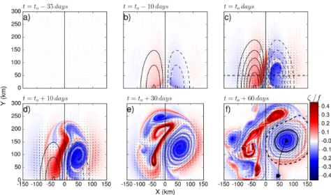
The temporal evolution of the response of the surface layer to a symmetric wind forcing corresponding to τo = 0.4 N m−2, To = 10 days and (W, L) = (40, 100) km is shown inFigure 4. These snapshots depict the non-linear evolution of the relative vorticityζ/f (colors) and the isocontours of positive (thin solid con-tours) and negative (thin dashed concon-tours) wind stress curl. Initially the layer thickness is at rest (a), then the wind forcing increases gradually until the wind stress reaches its maximum intensity (c). During this first period, the oceanic response follows roughly the symmetry of the wind forcing (Figure 4b). Anticy-clonic and cyAnticy-clonic oceanic vorticity are generated respectively on the anticyAnticy-clonic and the cyAnticy-clonic side of the wind jet. Once the wind forcing has reached its maximum intensityτo, an asymmetry in the oceanic response appears. The area of negative vorticity starts to spiral and form a large scale elliptical anticyclone (ellipticityε ∼ 0.5) while on the cyclonic side of the wind jet, the oceanic vorticity patch is stretched and strongly elongated (Figure 4d). Thirty days after the wind forcing has reached its maximum intensity ( Fig-ure 4e) there is no longer any atmospheric forcing and the oceanic layer evolves freely. One month later, we could consider that the oceanic layer reached a final stage with a fully developed mesoscale anticyclone having a quasi-circular shape (ellipticityε ∼ 0.19) and several smaller elliptical cyclones. The movie of this dynamical evolution (see supplementary materials) clearly shows that this final anticyclone remains robust and coherent with time while the smaller surrounding structures, especially the elongated cyclones, evolve quickly in time and are deformed in the strain field of the large anticyclone.

In order to quantify more precisely the dynamical characteristics of this large scale mesoscale anticyclone, we use the AMEDA automatic eddy detection algorithm to track and follow the evolution of its size, its intensity and its thickness. Figure 5shows the various stages of the evolution of the vortex radius Rmax, its maximal velocity Vmax, the relative isopycnal displacementλ and the relative vorticity ζ/f of the eddy core in addition with the ellipticityε of the characteristic contour. Almost all of these parameters follow the integral response of the wind stress curl, in other words the anticyclone accumulates the momentum and the energy transfered by the wind. We confirm here that the intensity and the depth of this robust and coherent anticyclone are reached shortly after the wind stops. On the other hand, the ellipticity reaches a quasi-steady state at least 1 month later (Figure 5f ) which indicates that the axisymmetrization of the wind induced anticyclone is an intrinsic mechanism which is not driven by the wind forcing. The typical size of the eddy seems to be also decorrelated to the wind forcing, since from the very beginning the characteristic radius is around Rmax ∈ 45 − 50 km and at the final stage it is estimated to be at Rmax = 46 km which is close to the width W = 40km of the wind jet. All the dynamical parameters of this specific wind induced anticyclone, namely its vortex Rossby number Ro = 0.07 and its Burger number Bu = 0.08, are in correct agreement with the robust mesoscale Ierapetra eddies that have radii two or three times greater than the deformation radius Rd(Ioannou et al.,2017).

Figure 4: Evolution of the relative vorticity fieldsζ/f (colors) of the ocean surface forced by a symmetric wind

hav-ing the followhav-ing characteristics (W, L) = (40,100)km, intensity τo= 0.4 N m−2 and duration To= 10 days (panels

(a-f )). The black contours indicate the location of the negative (dashed contours) and the positive (solid contours) wind stress curl applied in the top of the ocean layer. The characteristic contour (solid black line) and the last closed streamline (dashed black line), computed with AMEDA algorithm are shown for the final anticyclone in panel (f ). Sec-tion posiSec-tioned at a distance y = 50km away from the maximum forcing is represented with the dashed line in panel (c).

Figure 5: (a) Temporal variation of the wind forcing (Equation 9) for a characteristic time To= 10 d a y s. The evolution

of the dynamical characteristics of the large anticyclone, computed by the AMEDA algorithm, are shown in the panels (b) radius Rmax(km), (c) velocity Vmax(ms−1), (d) maximum isopycnal displacementλ, (e) the dimensionless core

vorticityζ(0)/f and (f) ellipticity ε.

4.2 Cumulative Impacts of the Wind Forcing and Its Duration: The Wind Forcing Parameter

During the first days of the wind forcing (Figure 4) the oceanic response follows the spatial pattern of the surface wind stress curl. As far as we consider seasonal wind variations, which evolve slowly (i.e. To−1¿ f ), we assume a quasi-steady response of the surface oceanic layer and use the steady Ekman pumping theory

Figure 6: Relative isopycnal displacementsη(x)/H (a) and dimensionless cross shore velocities v(x)/f W (b) of the

oceanic jet induced by the wind jet at y = 50km when the wind forcing is maximum (t = 0). The maximum wind forcing intensity isτo= 0.4 N m−2and the characteristic duration To= 10 days as inFigure 4. The values of the RSW

model (black line) are compared to the predictions of the steady Ekman pumping theory of Ekman (blue solid line) and Stern (blue dashed line).

(Ekman,1905;Stern,1965). The local wind stress curl will drive horizontal divergence and convergence of the Ekman transport and induce a vertical Ekman pumping velocity WE. The cumulative effect of the Ekman pumping leads to an isopycnal displacementηEthat is directly proportional to the wind stress intensityτo and its characteristic duration Towhile it is inversely proportional to the width W of the wind jet (Equation 13). ηE= t ˆ t0 WEd t = t ˆ t0 −1 ρ∇ × µτ f ¶ d t (13)

In order to take into account the relative vorticity of the oceanic current,Stern(1965) derives a non-linear relation to estimate the Ekman pumping induced by strong wind shears. The isopycnal displacement in-duced by the cumulative wind forcing is then given by the following relation

ηS= t ˆ t0 WEd t = t ˆ t0 −1 ρ∇ × µ τ f + ζ ¶ d t (14)

where t = t0is the beginning of the wind forcing,ρ the density of water and ζ the flow vorticity. This means that the Ekman transport will be enhanced in regions of anticyclonic vorticity and reduced in regions of cyclonic vorticity, already introducing an asymmetry in the ocean’s response.

At the initial stage of the wind forcing, before the formation of the non-linear dipole, we can assume that the wind jet will induce a unidirectional response in the oceanic layer. In other words, the wind jet will first induce an oceanic jet that ultimately destabilizes and generates a symmetric or asymmetric dipole. The

Figure 6a compares for the case shown inFigure 4, the isopycnal displacementsηE ,Spredicted by the linear and non-linear Ekman pumping (i.e. Equation 13andEquation 14) with the results of the RSW model. Since, in all of our simulations, the core of the initial dipole is formed 40 − 60km away from the coast, we estimate the isopycnal displacement at the distance y = 50km (dashed line inFigure 4c). Both the isopycnal displacementη(x) and the cross shore geostrophic velocity vg(x) =g

0

f∂xη are plotted at t = 0 when the wind jet reached its maximum intensity. The relative isopycnal displacementsλ = max(η)/H are quite large with an amplitude of 50% both in the cyclonic and the anticyclonic side. These values are accurately predicted by the steady Ekman pumping theory even if the standard Ekman formula (Equation 13) slightly overestimates

Figure 7: a) Maximum isopycnal displacementλ and (b) Rossby number of the oceanic jet Roj et reached at t = 0

(when the wind forcing is maximum) as a function of wind forcing parameterγ for various simulations. The black circles correspond to simulations performed with constant duration To= 10 d a y s while open square correspond to a

constant wind stressτo= 0.3 N m−2.

the displacement for the cyclonic part while the Stern formula slightly overestimate the displacement for the anticyclonic part. The numerical model confirms that the isopycnal displacement induced by the Ekman pumping is geostrophically balanced and that the cross shore velocities match the geostrophic velocity vg (Figure 6b). The Rossby number of the oceanic jet is quite small Roj et=max(v)f W ' 0.1. Hence, the non-linear effects of the Ekman pumping are negligible and therefore both Ekman and Stern predictions remain close, with errors less than 10%.

Since the initial response of the ocean to this seasonal wind variation is mainly driven by the Ekman pump-ing formula (Equation 13) we can use the latter to build a wind forcing parameter that quantifies the inten-sity of the oceanic response to the orographic wind jet. If we use theEquation 9(with c = 1) for the wind stress inEquation 13while considering that the wind forcing starts approximately at t0= −3 Towe get:

ηE(x) = 0 ˆ −3To − 1 ρ f ∂xτyd t = τo ρ f W2xe −12(x/W ) 2 0 ˆ −3To e−12(t /To) 2 d t ' τoTo ρ f W2xe −12(x/W ) 2 0 ˆ −∞ e−12ξ 2 dξ (15)

whereξ = t/T0is a dimensionless variable. Since the maximal isopycnal displacement is found at x ' ±W , we obtain: λ =max(η) H ' τoTo ρ f HW r π 2e (16)

We therefore introduce the dimensionless wind forcing parameter γ = τoTo

ρ f HW (17)

which quantifies the relative amplitude of the isopycnal displacement induced by the wind jet. We then investigate a wide range of parameters varying either the wind intensityτo or its characteristic duration To. We plot, inFigure 7for various wind forcingτo and various duration To, the maximum (positive) and minimum (negative) isopycnal displacement reached when the wind stress is maximum at t = 0. Positive (negative) isopycnal displacement refers to the anticyclonic (cyclonic) side of the oceanic jet flow. The black circles correspond to simulations performed with constant duration To= 10 d a y s but variable wind stress intensitiesτo, conversely open white squares illustrate simulations performed with constant intensityτo= 0.3 N m−2but various duration To. This graph confirms the linear relation between the dimensionless wind forcing parameterγ and the maximum isopycnal displacement λ of the surface oceanic layer. In agreement

with the Ekman (Equation 13) or the Stern (Equation 14) formula, finite values ofλ are obtained when γ is around unity. Large values ofγ correspond to strong wind intensity or long wind forcing duration. We also estimate the Rossby number of the oceanic jet Roj et=

Vj et

f W induced by the Etesian wind forcing.

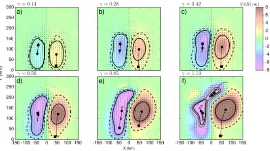
Figure 8: Snapshots of oceanic response to symmetric transient wind forcing for different wind stress intensities (a)

τo= 0.05 N m−2, (b)τo= 0.1 N m−2, (c)τo= 0.15 N m−2, (d)τo= 0.2 N m−2, (e)τo= 0.3 N m−2and (f )τo= 0.4 N m−2.

These sea surface heights (SSH) are shown 60 days after the maximum forcing occurs. The trajectories of the eddy centers are plotted with a black line. Black square indicates the beginning of each trajectory.

Once the maximum wind forcing is reached, the wind amplitude decreases slowly and after t = 3To the oceanic flow evolves freely. The destabilization of the oceanic jet leads to the formation of a free dipole which is more or less symmetric and propagates offshore. We illustrate inFigure 8the end state (t = 6To days after the maximum forcing) of the full non-linear flow evolution for different wind forcing parame-ters. To track and quantify the dynamical contours of the cyclonic and anticyclonic eddy of each dipole, we use the AMEDA eddy detection and tracking algorithm (Le Vu et al.,2018). The sea surface height and the characteristic contours (i.e. the streamline corresponding to the maximum eddy velocity) of these dipolar structures are plotted inFigure 8.

For relatively low value of the forcing parameterγ < 0.2, corresponding here to a maximum wind forcing lower than 7 m s−1, a quasi-symmetric dipole is formed. When the wind forcing parameter becomes finite (γ > 0.6) the asymmetry of the dipole becomes significant with a robust quasi-circular anticyclone and a strongly elliptical cyclone. If the shape of the anticyclone remains unchanged the cyclonic partner is often stretched and deformed by the strain field of the anticyclone and, for the most intense cases, it could even split in two or three smaller cyclones (Figure 8f ). Hence, when the wind jet is strong enough, in other words whenγ is around unity, a large and robust anticyclone is formed instead of a symmetric dipole.

In order to investigate how the wind forcing impacts the dynamical characteristics of the final eddies which are formed, we plot their dimensionless numbers as a function of the wind forcing parameterγ inFigure 9

andFigure 10, for the anticyclones and cyclones respectively. All the parameters associated to the eddy intensity, such as the vortex Rossby number Ro, the isopycnal displacementλ and the relative vorticity ζ(0)/f increase with γ. The strength of the initial Ekman pumping controls the intensity of the final eddies that remain once the wind forcing is over. However, unlike the initial oceanic jet, the intensity of the final anticyclones (the Rossby number and the relative core vorticity) saturate for finite values ofγ. On the other hand, the Burger number Bu =³ Rd

Rmax ´2

0 0.5 1 1.5 2 2.5 0 0.05 0.1 0.15 Bu a) 0 0.5 1 1.5 2 2.5 0 0.05 0.1 0.15 0.2 Ro b) 0 0.5 1 1.5 2 2.5 0 0.5 1 1.5 2 | | c) 0 0.5 1 1.5 2 2.5 0 0.1 0.2 0.3 0.4 0.5 | (0) f -1| d)

Figure 9: Dynamical characteristics of the final anticyclonic eddies estimated according to the AMEDA algorithm. The

Burger number Bu = (Rd/Rmax)2(a), the vortex Rossby number Ro = Vmax/( f Rmax) (b), the isopycnal displacementλ

(c) and relative core vorticityζ(0)/f (d) are plotted for various values of the wind forcing parameter γ. As inFigure 7the black circles correspond to simulations performed with constant duration To= 10 d a y s while open square correspond

to a constant wind stressτo= 0.3 N m−2.

0 0.5 1 1.5 2 2.5 0 0.05 0.1 0.15 Bu a) 0 0.5 1 1.5 2 2.5 0 0.05 0.1 0.15 0.2 Ro b) 0 0.5 1 1.5 2 2.5 0 0.5 1 1.5 2 | | c) 0 0.5 1 1.5 2 2.5 0 0.1 0.2 0.3 0.4 0.5 | (0) f -1 | d)

Figure 10: Same asFigure 9but for the cyclonic eddies. For comparison, the dynamical parameters of the anticyclonic eddies are plotted with the black crosses.

W = 40km. Since, the latter is large in comparison with the deformation radius Rd = 13 km, the Burger number is small and about³Rd

W ´2

' 0.1. Hence, the amount of potential energy contained in the anticyclonic (or cyclonic) eddies is much greater than the kinetic energy. As the wind forcing parameterγ increases, the radius of the vortex increases slightly and the corresponding Burger number decays. Therefore, the isopyc-nal displacementsλ could reach finite values even if the Rossby numbers remain moderate. This is a source of asymmetry between the cyclonic and the anticyclonic part of the wind induced dipole. There is indeed a physical limitation to the isopycnal displacement of cyclonic eddies. Whenλ reaches unity, the thickness of the surface layer will vanish in the core of a cyclonic eddy while there is no limitation for the anticyclonic structure. The anticyclonic core could strongly thicken if the lower layer is deep enough. This asymmetry is confirmed by theFigure 10c where the isopycnal displacements in the core of the anticyclones always exceed those of the cyclones. The isopycnal displacementλ is larger than unity only in the core of anti-cyclones for finite values of the wind forcing parameter. If we increase the wind forcing parameter above γ = 0.6 the upper layer thickness will almost vanish in the cyclonic eddies and numerical instabilities (i.e. shocks) will occur due to large values of the local Froude number. This is one of the main limitations of the rotating shallow-water model.

4.3 Asymmetric Forcing

We have seen, in the previous section, that a symmetric wind jet could induce an asymmetric dipole and, for finite value ofγ, the final stage could lead to a large and robust anticyclone having a quasi-circular shape. Although the climatological analysis of the Etesians (seeFigure 3) shows that this specific orographic wind jet is not symmetric but asymmetric. The anticyclonic wind shear is on average twice as strong as the cy-clonic shear and we naturally expect an asymmetric response of the oceanic surface layer. We therefore compare inFigure 11the oceanic response to a symmetric and an asymmetric wind jet having the same an-ticyclonic wind stress curl. The wind stress intensity is set toτo= 0.4 N m−2with a typical duration fixed by To= 10 days and we set the parameter c = 2 (Equation 11) for the asymmetric wind jet to mimic the Etesian winds. Because, the cyclonic shear is weaker, the cyclonic structure generated in the oceanic layer is sig-nificantly weaker for the asymmetric wind jet in comparison with the symmetric one. As for the symmetric case, coherent cyclonic eddies did not form and the weak cyclonic filaments are stretched and elongated. The reduction of the cyclonic wind shear also impacts the formation of the anticyclonic eddy. The final anticyclone is more circular (ellipticityε = 0.08) and slightly smaller (Rmax' 39 km) than in the symmetric wind forcing case whereε = 0.16 and Rmax' 46 km. Moreover, the vortex Rossby number of the anticyclone is 13% stronger. The cyclonic part of the dipolar structure being less intense, reduces the strain applied by the cyclone on the anticyclone and therefore the ellipticity of the latter. Besides, the self-advection of the asymmetric dipolar structure is also reduced and the anticyclonic eddy stays closer to the coast and the stronger winds, which amplify its intensity and limit its radial extension.

We also investigate the ocean response to increasing values of the wind forcing parameter γ. For such asymmetric wind forcing, the main oceanic response is a quasi-circular anticyclone which stays close to the coast and a linear trend is found between the eddy intensity (i.e. Ro,λ and ζ(0)/f ) and the wind forc-ing (Figure 12). Since, the cyclonic wind shear is weaker, the thickness of the upper layer will vanish in the cyclonic vorticity core for a stronger wind jet and we could reach higher intensity of the wind stress, up toτo = 0.7 N m−2, without numerical instabilities. The core vorticity of the anticyclonic eddy could then reach much higher values and will therefore satisfy the cyclogeostrophic balance. On the other hand, the eddy radius is weakly affected by the wind forcing and seems to be mainly controlled by the width W of the anticyclonic wind shear.

Figure 11: Symmetric and asymmetric wind stress curl applied to the shallow-water flow at the time of maximum

forcing are plotted in the upper left (a) and lower left (c) panels respectively. The cyclonic wind stress curl is two times smaller for the asymmetric (c) than for the symmetric case (a). The wind stress intensity isτo= 0.4 N m−2and the

forcing duration To= 10 days. The ocean responses to symmetric and asymmetric wind forcing are plotted in panels

(b) and (d), respectively. These relative vorticity fieldsζ/f correspond to the end state, t = 60 days after maximum forcing occurs. 0 0.5 1 1.5 2 2.5 0 0.05 0.1 0.15 Bu a) 0 0.5 1 1.5 2 2.5 0 0.05 0.1 0.15 0.2 Ro b) 0 0.5 1 1.5 2 2.5 0 0.5 1 1.5 2 | | c) 0 0.5 1 1.5 2 2.5 0 0.1 0.2 0.3 0.4 0.5 | (0) f -1| d)

Figure 12: Evolution of the Burger number Bu (a), the Rossby number Ro (b), the isopycnal displacement parameterλ

(c) and the relative core vorticityζ/f (d) as a function of the wind forcing parameter γ. These dynamical characteristics are estimated with the AMEDA algorithm for the final eddy state more than 30 days after the end of the wind forcing. As inFigure 9andFigure 10the black circles correspond to simulations performed with constant duration To= 10 d a y s

5 Intensification of a Preexisting Anticyclone by the Etesian Wind

Our previous work on the dynamical characteristics of IEs over a 22 years period (Ioannou et al., 2017) revealed that these large mesoscale anticyclones could be re-amplified, or in other words that they could gain a large amount of energy, one year after their formation. This intensification process coincides with the period of strong Etesian forcing. During such re-amplification stage, the intensity of the anticyclone could double in less than 4 months while keeping its mean radius almost unchanged. For instance, the Rossby number of the Ierapetra eddy formed in 1998 (IE98) varies from Ro = 0.08 in May 1999 to Ro = 0.16 in September 1999 (Ioannou et al.,2017). Similar re-amplification events were detected four times from 1993 to 2014.

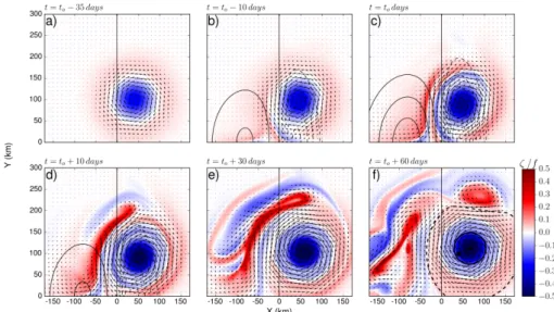
In order to verify that such re amplification phenomenon can indeed be induced by the Etesian wind forc-ing, we investigate the effect of the asymmetric wind jet (c = 2) on a pre-existing anticyclone. The latter is an isolated axis-symmetric Gaussian vortex, identical to the IE98 before intensification, with an initial radius Rmax= 40 km and Ro = 0.08. The anticyclone is located 100 km away from the coast at the position of the maximum negative wind stress curl (i.e. x = W ). TheFigure 13shows the dynamical evolution of this initial anticyclone forced by a wind jet intensity ofτo= 0.7 N m−2. The total duration of this varying asymmet-ric wind jet is about 60 days (seeFigure 5a when To= 10 d a y s). During the initial stage of the forcing, the oceanic jet induced by the wind, tends to roll up, around the center of the pre-existing anticyclone. Accord-ing toFigure 13c two bands of cyclonic and anticyclonic vorticity, spiral around the initial eddy core. The position of the latter is not modified even if its shape tends to be slightly elongated along the wind jet. Later on, after 30−40d a y s the negative vorticity filament tends to merge into the anticyclonic eddy core while the positive vorticity filament, which stays at the eddy periphery, splits into several smaller cyclonic structures

Figure 13e. A month after the wind has stopped (Figure 13f ), we get an intense and large, quasi-steady anti-cyclone on the right side and a mix of smaller unsteady structures of both signs on the left side of the initial wind jet. This specific wind forcing, which mimics the mean seasonal wind forcing, clearly re-amplifies the pre-existing anticyclone. The vorticity in the eddy core doubles fromζ(0)/f = −0.26 to ζ(0)/f = −0.6 while the vortex Rossby number increases by a factor of 2.25 and reaches the final value of Ro = 0.18 (Figure 14). The ellipticity of the anticyclone strongly varies during the wind forcing, but at the final state it recovers its initial value corresponding to a quasi-circular (ε = 0.015). The steepness parameter α changes from a Gaus-sian velocity profile (α = 2−2.2) to a more wide profile after the wind forcing reaches its maximum intensity (Figure 14f ) and reaches a steepness parameter ofα = 1.1 at the final state. More surprisingly, the radius of the vortex remains almost constant during the total simulation time slightly decreasing by 4% at the final state, reaching a radius of Rmax= 36 km. The characteristic eddy radius has the same scale with the applied wind forcing width and is the reason why no significant change in the eddy size is observed. This idealized example shows that the shape of a mesoscale anticyclone will be weakly affected by a local wind jet forc-ing while its intensity could strongly increase. The intensification phenomenon was also recovered when considering relative wind stress components. The impact of the current feedback on the wind forcing was found relatively small compared with the strong downwelling induced by the orographic wind stress curl (Appendix C). Such dynamical process is in correct agreement with the previous analysis of remote sensing AVISO/DUACS data set ofIoannou et al.(2017). Hence, the re-amplification of an IE can be explained by the seasonal orographic wind jet when the latter occurs over the pre-existing anticyclone.

Conversely, if a pre-existing cyclone is located below the positive wind shear, the initial eddy will be rapidly stretched and deformed, while an anticyclonic eddy will form on the right side of the wind jet (i.e. the negative wind-stress curl area). This example shown inAppendix Bconfirms the asymmetric response of mesoscale oceanic eddies to such orographic wind jet. Only large mesoscale anticyclones remain robust, quasi-circular and could gain energy from the Etesian winds in the southeast of Crete.

Figure 13: Evolution of the relative vorticity fieldsζ/f (colors) of an initial Gaussian anticyclone (Ro = 0.08 and

Rmax= 40 km) forced by a asymmetric wind jet (c = 2) having the following characteristics (W, L) = (40, 100) km,

in-tensityτo= 0.7 N m−2and forcing time To= 10 days. The black contours indicate the location and the intensity of the

negative (dashed contours) and the positive (solid contours) wind stress curl applied at the top of the ocean layer. The characteristic contour (solid line) and the last closed streamline (dashed line), computed with AMEDA algorithm are shown for the final anticyclone in panel (f ).

Figure 14: The evolution of the dynamical parameters corresponding to the intensified anticyclonic eddy of ( Fig-ure 13) are shown with the solid line in panels (a) eddy radius Rmax(km), (b) the maximal velocity Vmax(ms−1), (c)

the relative isopycnal displacementλ, (d) the dimensionless core vorticity ζ(0)/f , (e) the eddy ellipticity ε and (f) the steepness parameterα of the mean velocity profile (Equation 8) as computed by the AMEDA algorithm. The dynami-cal evolution of the generated anticyclone by the same wind forcing characteristics applied in an ocean initially at rest is illustrated with the dashed line.

6 Summary and Conclusions

In this study we investigated with a reduced gravity model, the mean oceanic response to a seasonal wind jet that varies slowly over several weeks or months. Motivated by the repeating formation and the intensifi-cation of the Ierapetra eddies in the southeast of Crete (Ioannou et al.,2017;Mkhinini et al.,2014), we study the relation between the intensity and the duration of the wind forcing and the dynamical characteristics of the wind induced eddies. The spatial structure of the mean wind jet was first established according to climatological wind data in order to mimic the Etesian winds blowing during summer between Crete and Kasos strait.

Even if the climatological wind jet is asymmetric, we started our analysis with a symmetric wind profile to understand the mechanisms responsible for the formation of a single large and intense anticyclone. Indeed, we found that, for a specific range of parameters, the oceanic response to a symmetric wind jet could be a strong asymmetric dipole which leads, when the wind forcing ends, to a single and intense anticyclone. The asymmetry of the oceanic response is mainly controlled by a dimensionless parameter that integrates in time the Ekman pumping. This wind forcing parameterγ quantifies the relative amplitude of the isopycnal displacement induced by the local wind stress curl. It is therefore proportional to the wind jet intensity and its duration but is inversely proportional to its width. Our analysis shows that for a small value of this wind forcing parameter, in other words when the isopycnal displacement remains weak, the oceanic response to a symmetric wind jet is a symmetric dipole. But, when the wind forcing parameter increases and gets close to unity, the isopycnal displacement becomes finite and the oceanic response is strongly asymmetric. This initial asymmetry can be explained by the drastic reduction of the upper oceanic layer for positive wind stress curl which prevents the formation of a large scale cyclone. On the other hand, there is no limit to the thickening of this layer when the wind stress curl is negative. Hence, the first response to an intense wind jet is an asymmetric dipole composed by a robust anticyclone and a strongly elongated cyclonic structure. When the wind forcing stops, this initial asymmetry increases due to the stretching of the cyclonic structure by the large and robust anticyclone. The latter becomes more circular as the initial cyclonic structure often divides into several smaller unsteady cyclones. Similar dynamical behavior was found by (Poulin and Flierl,

2003;Perret et al.,2006,2011) who studied the stability of oceanic jets or wakes flows. The asymmetry of these unsteady symmetric flows occurs in the cyclogeostrophic or the frontal regimes and tends to form large scale and robust anticyclones while the cyclones are stretched and elongated. In our case, the initial dipole induced by the orographic wind forcing can be seen as a localized oceanic jet. Since the width of this initial oceanic dipole is larger than the deformation radius, the Burger number Bu is small and even for moderate Rossby numbers Ro the localized oceanic jet will (i.e. the initial dipolar response) correspond to a frontal regime. Therefore, these two intrinsic mechanisms favor the formation of a mesoscale anticyclone when a large and strong wind jet blows perpendicular to the coast.

In a second step, we use an asymmetric wind jet having an anticyclonic wind shear two times larger than the cyclonic one to mimic the Etesian winds in this area. For this realistic configuration, intense mesoscale anticyclones that satisfy the cyclogeostrophic balance, as the real IE’s, could be formed. According to our analysis, the vortex Rossby number of these anticyclones evolve linearly with the wind forcing parameter γ, while the eddy radius remains almost constant and scales as the width of the orographic wind jet. For the strongest wind forcing, the final response of the surface layer corresponds to a single large scale and intense anticyclone surrounded by positive vorticity filaments and few sub mesoscale anticyclones. The typical Burger and Rossby numbers of these wind induced anticyclones obtained in our idealized simula-tions are compared with the most intense annual values of IE anticyclones estimated for several years of remote sensing analysis (Ioannou et al.,2017,2019) and from the DYNED-Atlas data base which provides 17 years of eddy detection and tracking in the Mediterranean Sea (https://doi.org/10.14768/2019130201.2). TheFigure 15shows that the size (i.e. Rmax/Rd eddy characteristic radius compared with the deformation radius) of the final anticyclones is in good agreement with the observations even if the intensity of the real IE’s seems to be somewhat higher that in our numerical simulations. Indeed, we didn’t succeed, with the simplified shallow-water model, to reach Rossby numbers higher than Ro = 0.18 or negative potential vor-ticity core (i.e.ζ(0) < −f in the eddy core) diagnosed by (Ioannou et al.,2017,2019). More realistic oceanic models which account for the vertical stratification and the mixed layer should be used to study the

com-plex wind eddy interaction and especially the turbulent ageostrophic structures that may emerge in the core of such intense anticyclones (Brannigan,2016;Brannigan et al.,2017).

Finally, we study how the seasonal variations of the Etesian wind jet impacts the dynamical characteris-tics of a pre-existing mesoscale anticyclone. In agreement with the remote sensing observations (Ioannou et al.,2017), the anticyclone remains robust and coherent, its intensity increases significantly while its ra-dius hardly varies. The Etesian wind forcing is therefore the main source of the IE’s intensification when the pre-existing IE is close enough to the orographic wind jet. Even if several studies (Horton et al.,1994;

Fusco et al.,2003;Mkhinini et al.,2014) have suggested that the IEs are forced by the Etesian winds, this paper is the first numerical study which provides a dynamical understanding for the formation of a single Ierapetra anticyclone in the southeast of Crete and explains its possible intensification one year after its for-mation. The numerical simulations also reveal that a strong submesoscale activity, with unstable filaments and intense cyclones, occurs on the cyclonic side of the wind jet when the Etesian reaches their maximum intensity. The formation of these submesoscale structures is enhanced by the asymmetry of the oceanic response, in other words when the mesoscale anticyclone is strong enough to stir and stretch the cyclonic side of the initial dipole. Unlike the IE’s, these submesoscale features cannot be accurately captured by satellite altimetry due to its coarse resolution. Moreover, regional models should also reach a minimum resolution to reproduce accurately these submesoscale patterns that may impact locally the Rhodes gyre during Etesian episodes.

0 1 2 3 4 5 Rmax/Rd 0 0.1 0.2 0.3 0.4 0.5 Ro 0 0.5 1 1.5 2 2.5 3 3.5 4 Lifetime (years)

Figure 15: Dynamical characteristics of the Ierapetra anticyclones illustrated with the squares based on (Ioannou et al.,2017) and with triangles from the DYNED-Atlas data base(https://doi.org/10.14768/2019130201.2). The vortex relative size Rmax/Rd and the vortex Rossby number Ro are plotted during the months were the eddies are more

intense. The lifetime of each detected anticyclone is depicted with the different colors. The black circles correspond to the retrieved anticyclones with the RSW model from all the performed simulations. The dimensionless wind forcing scale W /Rdused in the RSW model is illustrated with the orange dashed line.

A Estimation of the Oceanic Layer Thickness

In order to select a layer thickness that represents the seasonal stratification of the area, we estimate the climatology of the regional density profile. Argo profiles that cross the Ierapetra area from 2000 to 2015 are selected only if their position is detected outside of the last contour of an eddy based on AMEDA eddy and tracking detection algorithm (Le Vu et al.,2018). Based on these vertical profiles we obtain a mean seasonal density profile that could describe the unperturbed seasonal stratification in the region South-East of Crete (Figure A.1(a)). To build a two-layer stratification, having the same dynamical properties of a continuous stratification, we solve for the linear eigenmodes of the ocean’s vertical structure. The node of the first baroclinic eigenmode fixes the thickness of the upper and the lower layer for the equivalent two-layer system. According toFigure A.1, the characteristic thickness of the upper layer is estimated at H = 100m. ∂ ∂z f2 N2 ∂ ∂zφn+ 1 R_d2φn = 0 (A.1) with ∂φn ∂z = 0 at z = 0, H 0 0.2 0.4 0.6 0.8 1 / max -0.4 -0.35 -0.3 -0.25 -0.2 -0.15 -0.1 -0.05 0 z/H

a)

b)

c)

Figure A.1: (a) Mean climatological densityρ profile as computed from ARGO floats that we detected outside from an

eddy from 2001-2015 and the associated Brunt-Väisälä frequency in (b). (c) The first mode of the baroclinic structure of the ocean for the region of Ierapetra.

B Asymmetric Wind Forcing Above Preexisting Cyclone

We illustrate in this section the effect of a transient asymmetric wind forcing applied above a pre-existing cyclonic eddy. For that purpose a cyclonic eddy of Rmax = 30 km and vortex Rossby number Ro = 0.05 is initialized respectively in the positive side of the wind stress curl as shown inFigure B.1(left panel). The eddy is subject to an asymmetric wind forcing of intensityτo= 0.3 N m−2and duration of To= 10 days. The non-linear evolution of the flow is depicted inFigure B.1(right panel) at time t = 60 days, after the maximum forcing has occurred. In the presence of the positive wind stress curl the cyclonic eddy does not retain its shape. At the final state the cyclonic eddy is stretched and elongated in cyclonic filaments. Contrary on the negative side of the wind stress curl as expected a new anticyclonic eddy is formed. Thus only mesoscale anticyclones could be re-amplified while remaining robust under the influence of a negative wind stress curl.

Figure B.1: Asymmetric wind forcing with characteristics (W, L) = (40,100)km, intensity τo= 0.3 N m−2and duration

To= 10 days as shown in panel (a) at the time of maximum forcing (t = 0) is applied above a cyclonic eddy of initial

characteristics Rmax = 30 km and Rossby number Ro = 0.05. The vorticity fields ζ/ f of the oceanic response are

illustrated at t = 60 days after the maximum forcing in panel (b).

C Relative Wind Forcing

We evaluate in this section, how the current feedback on the wind forcing may modify the generation and the intensification of eddies by the Etesian winds. The current feedback effects arise in the wind stress forcing when accounting for the relative velocity between the wind and the ocean. The relative wind stress vectorτ = (τx,τy) acting on the ocean surface can be then estimated from the bulk formula as:

τ(x, y,t) = ρai rCd|U|U (C.1)

whereρai r= 1.2 kg m−3is the air density, Cdthe drag coefficient (here constant Cd= 3 10−3) and U = uw− ue the relative wind vector defined as the difference between the surface wind uwand the surface oceanic ue velocities. The wind velocity is along Oy direction and depends only on x: VW(x) and therefore the relative wind velocity is (u = −ue, v = VW−ve). The Ekman pumping driven by the relative wind stress curl will write as: WE = 1 ρoceanf ∇ × τ = 2ρai rCd ρoceanf [VW∂xVW− VW∂xve− ve∂xVW+ ve∂xve− ue∂yue] (C.2) Based on the standard theory, the oceanic velocities ueare neglected and the wind stress acting on the ocean surface depends only on the wind forcing speed VW. Thus the induced wind stress curl will be a result only of the imposed orographic wind shear that will drive a strong downwelling of the isopycnals (WE =

1

ρoceanf ∇ × τ = 2 ρai rCd

ρoceanf[VW∂xVW]). The amplitude of the induced Ekman pumping in this case, considering the Etesian orographic spatial shape ofEquation 9at the position of the maximum wind stress curl x = ±W , will scale as:

W_Est and ar d(x = W ) = − τo ρoceanf Wpe ' −ρai rCd ρoceanf V_o2 W = − ρai rCd ρocean RoW_{j et}Vo (C.3)

where RoW_{j et}= Vo

f W is the Rossby of the wind jet that is proportional to Vo, the maximum wind speed at the core of the jet and inversely proportional to its width W .

Contrary, when eddies are present in the oceanic fields, the current feedback will contribute, at the first order, to an opposite Ekman pumping (Equation C.2). Indeed, if we consider a uniform wind forcing acting above a Gaussian shape anticyclone (described byEquation 8), a positive Ekman pumping will be induced at the eddy center x = 0 (∇ × τ = ∂xτy = 2 ρai rCdVW∂xve). The upwelling of the isopycnals will mainly depend on the wind intensity Voand the eddy vortex Rossby number Ro

W_EF eed back(x = 0) = +2 ρai r ρoceanf CdVo Vmax Rmaxpe ' ρai r ρocean CdVoRo (C.4)

Compared with the standard Ekman pumping, the relative Ekman pumping will be reduced. The ratio between negative and positive Ekman pumping (Equation C.5) is mainly controlled by the Rossby of the eddy Ro and the Rossby of the wind jet RoW_{j et}.

r =W f eed back E W_Est and ar d = Ro RoW_{j et} (C.5)

For the range of parameters of the Etesian orographic wind forcing we are considering, the typical Rossby number of the wind jet ranges between RoW_{j et}∈ 1 − 3 (corresponding to wind velocities of Vo∈ 5 − 15 ms−1). On the other hand the typical eddy intensities for the Ierapetra anticyclones are between Ro ∈ 0.1 − 0.3, being one order of magnitude smaller. Thus the feedback effect on the driven Ekman pumping velocities is expected to be relatively small (of the order of 10 − 30%).

In order to quantify more precisely the feedback effect on the generation and the intensification of eddies we perform simulations taking into account the relative winds. In accordance withFigure 14, we evalu-ate the oceanic response subject to a asymmetric wind forcing of intensityτo = 0.7 N m−2 equivalent to wind intensity of Vo = 14 m s−1 and duration of To= 10 days and in the presence of an anticyclonic eddy of Rmax = 40 km and vortex Rossby number Ro = 0.08. We compare inFigure C.1the dynamical charac-teristics of the intensified eddies in the standard and in the feedback case. In the latter, a reduction of 12% and 18% was found in the eddy velocities and core vorticity respectively at their end state (6 To after the maximum forcing). Compared with the standard intensification, the isopycnal displacements were found slightly weakened (by 6%) while the radius of the intensified eddies remained relatively the same. The gen-eration of eddies with the relative winds was also investigated for the same wind forcing characteristics. In that case a reduction of 8% and 17% was found in the eddy velocities and core vorticity respectively between the generated anticyclones.

In agreement with the scaling analysis, the feedback effect on the driven Ekman pumping velocities re-mained below 20%. The strong negative wind stress curl imposed by the orographic Etesian wind forcing overcomes the positive wind stress curl driven by the wind-ocean interactions recovering the generation and intensification of strong and coherent anticyclones.

Figure C.1: The vorticity fieldsζ/f of the oceanic response are illustrated for the standard wind stress in panel (a)

and for the relative wind stress in panel (b) at t = 60 days after an asymmetric wind forcing of spatial characteristics (W, L) = (40,100)km, maximum intensity τo= 0.7 N m−2and duration To= 10 days was applied in the presence of an

anticyclonic eddy of characteristic radius Rmax= 40 km and Rossby number Ro = 0.08. The evolution of the

dynam-ical parameters for the two anticyclonic eddies, computed by the AMEDA algorithm, are shown in panels (c) radius Rmax(km), (d) velocity Vmax(ms−1) and (e) Maximum isopycnal displacement λ for the standard case (solid lines)

and the feedback case (dashed line).

Data Availability Statement

The data used in this study can be obtained online at doi:10.5281/zenodo.3523083 repository. The AL-ADIN datasets used in the current work can be downloaded from the Med-CORDEX database (www. med-cordex.eu). The DYNED-Atlas data base for the Mediterranean Sea is available athttps://doi.org/10.14768/ 2019130201.2.

Acknowledgments

This work was supported by the TOEddies CNES-TOSCA research grant and the ANR-Astrid Project DYNED-Atlas (ANR-15-ASMA-00 03-01).

References

Bakun, A. and Agostini, V. N., (2001) ““Seasonal patterns of wind-induced upwelling/downwelling in the Mediterranean sea"” . SCIENTIA MARINA, 65(3):243–257. doi:10.3989/scimar.2001.65n3243.

Barton, E., Basterretxea, G., Flament, P., Mitchelson-Jacob, E., B.Jones, Aristegui, J., and Herrera, F., (2000) ““Lee region of Gran Ca-naria"” . Journal of Geophysical Research, 105:17173–17193.

Brannigan, L., (2016) ““Intense submesoscale upwelling in anticyclonic eddies"” . Journal of Geophysical Research Letters, 43:3360–3369. doi:10.1002/2016GL067926.