Validation of O(¹S) wind measurements by WINDII: the WIND Imaging Interferometer on UARS

HAL Id: hal-01627421

https://hal.archives-ouvertes.fr/hal-01627421

Submitted on 6 Feb 2021

HAL is a multi-disciplinary open access

archive for the deposit and dissemination of

sci-entific research documents, whether they are

pub-lished or not. The documents may come from

teaching and research institutions in France or

abroad, or from public or private research centers.

L’archive ouverte pluridisciplinaire HAL, est

destinée au dépôt et à la diffusion de documents

scientifiques de niveau recherche, publiés ou non,

émanant des établissements d’enseignement et de

recherche français ou étrangers, des laboratoires

publics ou privés.

Validation of O(1S) wind measurements by WINDII: the

WIND Imaging Interferometer on UARS

W. A. Gault, Gérard Thuillier, G. G. Shepherd, S.-P. Zhang, R. H. Wiens, C.

Tai, B. H. Solheim, Yves Rochon, C. Mclandress, Chantal Lathuillière, et al.

To cite this version:

W. A. Gault, Gérard Thuillier, G. G. Shepherd, S.-P. Zhang, R. H. Wiens, et al.. Validation of

O(1S) wind measurements by WINDII: the WIND Imaging Interferometer on UARS. Journal of

Geophysical Research: Atmospheres, American Geophysical Union, 1996, 101 (D6), pp.10405-10430.

�10.1029/95JD03352�. �hal-01627421�

JOURNAL OF GEOPHYSICAL RESEARCH, VOL. 101, NO. D6, PAGES 10,405-10,430, APRIL 30, 1996

Validation of O(S) Wind Measurements

by WlNDII:

the WIND Imaging Interferometer on UARS

W.A. Gault,

• G. Thuillier,

2 G.G. Shepherd,

• S.P. Zhang,

1 R.H. Wiens,

• W.E.

Ward,

a C. Tai, a B.H. Solheim,

1 Y.J. Rochon,

1 C. McLandress,

a C.

Lathuillere,

4 V. Fauliot,

2 M. Hers•,

2 C.H. Hersom,

a R. Gattinger,

s L. Bourg,

2

M.D. Burrage,

6 S.J. Franke,

7 G. Hernandez,

s A. Manson,

9 R. Niciejewski

6

and R.A. Vincent. to

Abstract. This paper describes the current state of the validation of wind

measurements

by the wind imaging

interferometer

(WINDII) in the 0(1S)

emission. Most data refer to the 90-to-l10-km region. Measurements from

orbit are compared with winds derived from ground-based observations using

optical interferometers, MF re[de[rs and the European Incoherent-Scatter radar

(EISCAT) during overpasses

of the WINDII fields

of view. Although the data

agreement for the zero reference between the winds measured on the ground

and those obtained from orbit. A comparison with winds measured by the

high resolution

Doppler imager (HRDI) instrument

on UARS has also been

made, with excellent results. With one exception the WINDII zero wind

reference

agrees

with all external measurement

methods

to within 10 m s -•

large station-to-station differences. The subject of WINDII comparisons with

MF radar winds requires

further study. The thermospheric

O(•S) emission

region is less amenable to validation, but comparisons with EISCAT radar

data give excellent agreement at 170 km. A zero wind calibration has been

obtained

for the O(•D) emission

by comparing

its averaged

phase

with that

for 0(1S) on several

days

when alternating

1D/•S measurements

were made.

Several other aspects of the WINDII performance have been studied using

data from on-orbit measurements. These concern the instrument 's phase

stability, its pointing, its responsivity,

the phase distribution in the fields of

view, and the behavior of two of the interference filters. In some cases, small

adjustments have been made to the characterization database used to analyze

the atmospheric data. In general, the WINDII characteristics have remained

very stable during the mission to date. A discussion of measurement errors

is included in the paper. Further study of the instrument performance may

bring improvement, but the utimate limitation for wind validation appears to

be atmospheric variability and this needs to be better understood.

•York University, Toronto, Ontario, Canada.

2 Service d'A•ronomie du CNRS, Verri•res-le-Buisson, France. 3Institute for Space and Terrestrial Science, Toronto, Ontario,

Canada.

4 Centre d'Etude des Ph•nom•nes Aleatoires et G•ophysiques,

Saint-Martin-d'H•res, France.

S National Research Council, Ottawa. 6University of Michigan, Ann Arbor. ? University of Illinois, Urbana. 8 University of Washington, Seattle. øUniversity of Saskatchewan, Saskatoon.

•øUniversity of Adelaide, Adelaide, Australia.

Copyright 1996 by the American Geophysical Union.

Paper number 95JD03352.

0148-0227/96 / 95 JD-03352505.00

1. Background

The wind imaging interferometer (WlNDII) was put

into orbit on NASA's Upper Research Satellite (UARS)

on September 12, 1991. Its mission was to measure

winds, temperatures, and emission rates in the altitude range 80 to 300 km, with an emphasis on the lower part of this range. Nearly 16 million images of the upper atmosphere had been acquired up to November 1994, and analysis of the data is in progress. Validation of

the results is an essential part of this. In this paper we describe the validation process that was conducted

in order to give the reader, including future users of WlNDII data, an understanding of the procedures that

were employed. Also included is a description of the er-

ror estimate procedures and estimated error values. A

detailed description of the comparison with a ground- based Michelson interferometer is presented in a com-

panion paper by Thuillier et al. [this issue]. Prelimi-

nary scientific results have been presented by Shepherd

et al. [1993a], McLandress et al. [1994], and Shepherd

et al. [1995]. The present paper describes the current

state of the validation of the winds measured from the

O•S emission and the method used to determine the

preliminary zero wind value for the O•D wind measure-

mcnts. The validation of other quantities measured by

WINDII will bc presented in later publications. The instrument has bccn described by Shepherd et al.

[1993b], along with the basic data analysis procedure.

A field-widened Michelson interferometer [Hilllard and

Shepherd, 1966] is positioned in the optical path of a

charge coupled device (CCD) imager directed toward

the Earth's limb with the bottom of the image corre- sponding to a tangent point altitude of about 80 km and the top at about 300 kin. Single airglow emission lines arc isolated with interference filters, so that an image obtained from that emission is an image of the emission

rate multiplied by the transmittance of the interferome-

ter, which depends on its phase setting as well as on its

off-axis phase variation. One mirror of the interferom-

eter is phase stepped as an image sequence is acquired, either four or eight steps to cover one complete fringe. For each pixel on the image the corresponding eight sig-

nal values arc analyzed to determine the phase of the

cosinusoidal signal. The principle of wind measurement from space consists of comparing the phase generated by an airglow linc with the phase in the same instru-

mental condition when there is no Doppler shift of the

wavelength of this line. Let the •b be the phase of the

emission between 0 and 2•r and let •bint bc this intrinsic phase when the wind is null. The wind velocity is then

given by v: K• (•b - •bint), where K• is the constant

•oC Hcrc Ao is the unshiftcd

wavelength

of the cmis-

27rD ' '

sion, c is the velocity of light, and D is the effective optical path difference of the interferometer as given by

Thuillier and ttersd [1991].

As the zero wind phase is not available in orbit, a

calibration lamp delivering a line of wavelength close to A0 is used, providing a phase •c. Calibration on the ground consists in measuring •i•t - • by the use of the same lamp as in orbit and a source delivering the same airglow line as in the Earth's atmosphere. The fundamental principle of the wind measurement is to

assume that

(0int -- O

c)orbit

= (0int -- O

c)ground

----

Oz

(1)

95• is assumed to be a constant from ground to space. It needs to be known for the two instrument fields and for both day and night apertures. Operating the cali-

bration lamp at regular intervals in orbit provides 95•,

allowing the reconstruction of the zero wind phase in or-

bit from 95• + 95• and its trend during the mission. The

purpose of the validation is to estimate the magnitude

of the errors, and this is discussed in detail below.

In practice, it is more complicated than this. First

of all, since wc arc dealing with images, •int is an im-

age •bint(k,/), where k and 1 represent CCD rows and

columns, respectively. In addition, WINDII has two

fields of view, one at 450 and the other at 1350 to the spacecraft velocity vector, in order to measure two com- ponents of the horizontal wind; the fields of view have

independent

•bint(k,

1)• and •bint(k,

1)2 images.

As well,

WINDII uses a stopped-down aperture during the day-

time to accommodate the baffle system which screens

the light from the bright cloud

tops below. Since

only a

portion of the full Michelson interferometer aperture is

used in this case, the phase condition is different from

that at night, and so there arc two different

zero images

for each

field

of view,

e.g.,

qbint(k,

1)2

D and qbint(k,

1)2

N for

field of view 2 (FOV2). Finally, the spacecraft

velocity

component along the line of sight must bc removed, as

well as that of the Earth's rotation velocity.

The WINDII instrument

has an extensive

package

of calibration equipment, intended to provide a basic

characterization capability in orbit. This includes four spectral lamps for phase calibration in each of the four

spectral regions, a tungsten lamp for responsivity cali-

bration

and a laser

for the calibration

of visibility,

which

is a measure of the intcrfcromctcr's ability to modulate

emission lines. The stabilized Hc-Nc laser is in itself a primary standard of visibility.

The spectral lamps and the tungsten lamp arc consid-

ered secondary standards that wcrc calibrated against

primary standards on the ground. The primary stan-

dards for phase (zero wind) were laboratory lamps emit-

ting the same atmospheric emission lines as observed in flight. Prcfiight ground characterization also included measurement of the filter passbands for each elementary

bin on the CCD.

In addition to showing general consistency with other

methods of measuring the wind, there wcrc several spe-

cific reasons to conduct in-flight validation of the data.

Calibration measurements arc particularly difficult with

an interferometer having a large field of view, and there

is the possibility of sudden changes occurring during launch and gradual ones afterward in the space envi- ronment. The laboratory sources of atmospheric lines could have had undetected parasitic lines able to in- ducc some systematic phase error. Also, only one of

the two instrument fields of view was calibrated with

the atmospheric linc source, and this calibration was

then transferred to the other field, assuming symmetry in the interferometer. This procedure may have intro-

duced some error. Atmospheric observations made at

the Earth's limb require the deconvolution of one or sev- eral integral equations as a function of altitude. In the case of WINDII, three equations are solved by a method

explained by Shepherd et al. [1993b]. All of the above

considerations led to the necessity of having a campaign

of correlative measurements between WINDII in orbit and other instruments.

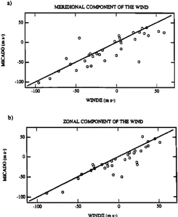
Important comparisons were made with a similar

GAULT ET AL.: WINDII VALIDATION 10,407

line, the MICADO instrument operated at the Obser- vatoire de Haute-Provence. Other optical comparisons

were made with the same emission line but against a dif-

ferent type of instrument, Fabry-Perot interferometers operated at Mount John in New Zealand and at Peach Mountain in Ann Arbor, Michigan. Another type of

comparison was made with the high-resolution Doppler

imager (HRDI) on UARS [Hays et al., 1993], which

measures winds from a different emission, the 02 atmo-

spheric band. Finally, comparisons were made against

measurements by nonoptical methods, namely, radars. There is an extensive worldwide network of MF radars, and for these comparisons, sites were selected in Ade- laide, Christmas Island, Saskatoon, and Urbana. In ad-

dition, the European incoherent-scatter (EISCAT) fa-

cility provided incoherent scatter wind comparisons, in-

cluding an important one at 170 km. All of the WlNDII

data reported here have been analyzed using version 4.23 of the production software.

2. Wind Measurement Procedure 2.1. Instrument Description

Light entering WINDII passes first through a large

(•1 m) baffle, then through a telescope, a filter,

other telescope, the Michelson interferometer, and nally is focused at the CCD detector by a camera lens. The first telescope has two objective lenses and a dou-

ble mirror which combines the two fields of view into

one, so they appear side by side on the CCD. The sec- ond telescope contains the actual field stop. The filter

wheel has eight positions, one of which is open to allow for calibrations and the imaging of star fields. The other seven positions contain interference filters for the var- ious atmospheric emissions and background measure- ments. Several plane mirrors are used to fold the optics

into a compact form. The look directions for the two

fields of view are approximately normal to each other,

viewing the atmosphere at the limb on the antisunward

side of the spacecraft, at 450 and 1350 to the velocity

vector. Diagrams of the instrument and optical system

are given by Shepherd et al. [1993b].

During calibrations, two mirrors are deployed, one in front of each entrance aperture and at 450 to the optical axis, cutting off light from the atmosphere and allowing the instrument to view the calibration sources. Phase calibrations and dark current measurements are done approximately every 15 to 20 min. Major calibra-

tions, including responsivity (tungsten lamp) and visi-

bility (He-Ne laser) as well as phase

(spectral

lamps),

are done about once per week.

The baffle is designed to permit daytime measure- ments of the weak airglow emissions, which can appear as closely as 1.50 above the sunlit cloud layers. This design includes a retractable stop which reduces the en- trance aperture to a narrow slot during the daytime in order to prevent the sunlight scattered by the cloud lay- ers from entering directly into the WINDII optical sys-

tem. We refer to these two configurations as the "day

aperture" and the "night aperture". The reduced col- lecting area during the daytime is approximately com- pensated by the increased emission rate.

The Michelson interferometer is achromatically field widened and thermally compensated and set at a path difference of 4.46 cm. With a larger path difference than this, the fringes due to the hot thermospheric emissions

(O 1D and O + 2p) would lose visibilty and their wind

measurements would be compromised. The Michelson

consists of hexagonal beam splitter and two arms of different glasses with a small gap at the end of one arm.

The mirror in this arm is piezoelectrically mounted for

alignment adjustment and changing the path difference

in the small steps required to measure the phase and

visibility of the fringes. The whole interferometer is cemented together, forming a very rugged unit.

To limit the amount of data for transmission and

improve the signal-to-noise ratio, the CCD pixels are

grouped together in bins and the signals are added on the chip for each bin. Most measurements are made us- ing six columns of bins, each 25 pixels wide and 2 to 8

pixels high. Observing windows are also defined for the CCD, including only the parts of the CCD where useful

data are obtained. The fields of view are fixed with re-

spect to the spacecraft, so the emission layers rise and

fall in the CCD image as the spacecraft

changes

alti-

tude, and the windows

move

up and down accordingly.

Typical exposure times for the iS emission are 1 to 2 s.

2.2. Data Analysis

Analysis of WINDII data begins at the level of the

individual bins which compose the phase images. Each

bin measures a line-of-sight intensity of the airglow

limb. The altitude associated with a bin is the alti-

tude at the tangent point. Thus a column of bins scans

a vertical slice in the atmosphere with an altitude range

defined by the bottom and top bins in the column. The horizontal extent is normally the full width of the im-

age area, which maps to about 140 km at the tangent

points along a row of bins. A single pixel subtends ap-

proximately

1 km 2 at the tangent

point giving

a vertical

resolution of 2 km for a two-pixel bin. The bin size is

chosen to give optimum signal to noise ratio and spa-

riotemporal resolution for a given observation.

A measurement contains the atmospheric signal as

well as a background signal. During normal opera-

tions a background image is taken followed by a set

of phase images. The processing software subtracts the appropriate dark current from the background and at- mospheric images bin by bin. The raw count rate is next

converted to geophysical units (Rayleigh) using the re-

sponsivity of each bin. (One Rayleigh corresponds to an

emission

of 10

• photon

s -1 from a 1 cm

• column

along

the line of sight.) This calibration information is stored

in a characterization database (CDB) which is accessed

by the production processing software. Since the back-

than the atmospheric line of interest, the background image is corrected to the observation wavelength. The method used to correct the background image is de-

scribed by Shepherd et al. [1993b]. The corrected back-

ground is then subtracted from each of the measurement images yielding only the atmospheric signal.

WINDII views the limb and so is sensitive to the

spacecraft attitude. The altitude, latitude, and longi- tude of each bin in each image are computed. Either four or eight images are taken for a normal measure- ment. The observatory may roll or change attitude from image to image. Using a middle image in a set of 4 or 8 to give a reference altitude, the remaining images are

corrected to account for any attitude variation. Next the velocities due to spacecraft motion and earth rota-

tion, projected along the line of sight, are derived for

each bin. These are used to calculate the contribution

to the observed phase of the spacecraft-induced Doppler

shift. The instrument phase determined from the fre-

quent phase calibration is corrected from the CDB to give the zero wind phase for the current measurement. Finally the projected velocity phase and the zero wind

phase are combined with the mirror step phase to give

the known phase component of the measurement.

The measured intensity of a given bin at a given time may be written in the generalized form as an integral along the line of sight L:

E(z)

[1

+ VV(z)cos((I>p

+ &w

(z))]

dl

(2)

where E(z) is the volume emission rate at altitude z, U

is the intrinsic (instrumental) visibility of a given bin,

V(z) is the line visibility corresponding to the atmo-

spheric temperature, T(z) and Ow(Z)is the phase due

to the atmospheric wind; (I>p -• + (p-•)•o, where • is

the phase due to the optical path difference, spacecraft velocity, and Earth rotation, •o is the step size for the Michelson mirror, and the index p- 1,2,...,n, where n is the number of steps per measurement. Usually,

90 _ 2__=.

The relationship

between

V(z) and T(z)is

given by

V(z)-

(a)

where A is the optical path difference in the interferom-

eter and Q is a molecular constant [Hilllard and Shep-

herd, 1966].

If the cosine argument is expanded, then equation (2)

may be written as

- Z(z

+ v cos Z(z)V(z)

cos(Ow(Z))a

- Usin

(I>p

E(z)V(z)sin(Ow(z))dl

Ip : J• n t- U COS (I)pJ2 - U sin (I)pJ3 (5)

The values J•, J2, and J3 are the line integrals in

equation (4) and contain the atmospheric information

we wish to recover. The vectors J•, J2 and Ja are de-

fined to be the "apparent quantities." Equation (5)

thus forms a simple linear system which is solved with standard matrix techniques.

Wave motion, or other structure in the atmosphere,

perturbs the interferogram and thus introduces error

in the recovered wind. The magnitude of this error is reduced by combining the six columns in a typical image across each row to give one vertical column or one

profile for each field of view. This column combination

also reduces the random error relative to a single bin. The final result provides two column vectors referenced to the centers of each field of view for each of J•, J2, and Ja. These are the apparent quantities that are used

in the inversion routine.

A locally spherically uniform and time invariant at- mosphere is assumed for the inversion of the apparent quantities; the inversion might not correctly recover the atmospheric information in regions of significant inhomogeneity, for example, in twilight or in regions of auroral activity. Each profile for each field of view is inverted separately using a linear constrained least

squares method with statistical weighting [MenIce, 1984;

Twomey, 1977]. Linear constraints are introduced for

damping noise-related oscillations. Data reduction, in- cluding the inversion process, is further summarized in

section 3 within the context of a random error assess-

ment. There is always a trade-off between noise re-

duction and the smoothing of vertical structures. The weighting factors and the constraint matrices have been

chosen to reduce noise but not to remove real atmo-

spheric structure.

Once the volume emission rate, wind, and tempera- ture profiles have been obtained from each field of view, the meridional and zonal wind components are derived by combining forward and backward looking observa- tions. The two fields of view track each other through

the atmosphere. Approximately 7 min after the forward

field of view sees a particular volume of air, the back- ward looking view sees the same volume from a perpen- dicular direction. The line of sight winds are combined to yield the vector winds only if the two views inter- sect within 300 km at the tangent points. The volume

emission rate and the wind from the two fields are aver-

aged to give the final profiles at the intersection point. Before averaging the scalar quantities or resolving the wind vectors, the profiles are all interpolated to a com- mon altitude grid. The final step in the processing is to reduce random noise without removing discernible

atmospheric structures.

2.3. Instrument Characterization

The ground characterization of WINDII took place during September and October, 1990, approximately

GAULT ET AL.' WINDII VALIDATION 10,409

one year prior to launch. This was an effort to measure

all the characteristics of the instrument that would be

needed to create the CDB, which is used to support op-

erational data processing. A full discussion of the char-

acterization is given by Hersom and Shepherd [1995].

Among the quantities measured were the zero reference

phase for O1S and the responsivity.

A small laboratory source of O1S emission was de-

veloped by Resonance Incorporated, to determine the interferometer 's phase corresponding to zero Doppler

shift. The limitations of the low intensity of the 557.7-

nm emission and the need to block a nearby contam-

inant line meant that the entrance aperture could be

fully illuminated for only a portion of the field of view.

Thus the zero was determined for a region near the bottom of the field, and a rubidium lamp, with an iso- lated emission line at 557.9 nm, was used to provide the

phase distribution over the rest of the field as well as

the phase shift between day and night aperture settings. In addition, phase measurements were made using the

onboard krypton calibation lamp (557.0 nm) so that

(•bint- •bc)ground

could

be determined

for O1S.

No lab-

oratory source was available for the O•D emission at

630.0 nm, but the phase distribution over the field and

the difference in phase between day and night apertures

was determined using the neon line at 630.5 nm. The responsivity measurement utilized a calibrated tungsten-halogen lamp to irradiate a barium sulfate re-

flectance screen placed in front of the instrument in such

a way that both the aperture and the field of view were completely filled. The lamp was located about 8 m from the reflectance screen to ensure good uniformity of illu-

mination. For each interference filter and both aperture positions a series of exposures was taken with the inte-

gration time incremented by 0.25 s from 0.25 s to the

saturation point. This provided about 10 measurements for each case. For these measurements the signal was

integrated in standard CDB bins of 1 x5 pixels, with the long sides horizontal. Thus each image consisted of 240

rows and 31 columns of bins in each of the two fields of

view. A least squares linear fit was applied to each data set to determine the signal versus exposure coefficient for each bin. The light level illuminating the aperture was computed in Rayleigh from the known transmission characteristics of the filter, the reflectance of the screen, and the lamp calibration. The instrument responsivity

was then determined in ADU s -• Rayleigh -1, where an

ADU (analog-to-digital unit) corresponds to one level

of digitization.

3. Wind Random Error Assessment

3.1. Introduction

WINDII data provided in the UARS database contain information on the precision of the wind measurements.

In this section the sources of random errors in the de-

termination of WINDII winds are reviewed. For clarity,

errors affecting the line of sight or apparent quantities

are first discussed followed by a summary of the errors associated with the inverted quantities. This approach

provides an understanding of the physical sources and

causes of the errors which would be masked if only in-

verted quantities were discussed.

The quantity directly measured by WlNDIi is a line

of sight emission rate (integrated through the emission

layer) modulated by the interferometer. The line of

sight or apparent phase is calculated by solving a matrix equation formed using sequences of these line of sight

modulated emission rates. The associated inverted

quantities are calculated from the apparent quantities using linear constrained least squares inversions with statistical weighting, as described in section 3.3. Asso- ciated with the derived quantities resulting from each of these steps is a statistical uncertainty in the derived quantitity. These are termed random errors. Apart from the inverted quantities, the variances of these er- rors are calculated, using standard methods, from the

error variances of the variables on which the derived

quantity is dependent. More formally, for any solution

vector quantity, f = f(xi), dependent on vectors xi, the

expression

f -- • q-

• Disi

(6)

i

follows from a first-order expansion of f in terms of the

xi. Here, f is an appropriate reference value for f, the Di are coefficient matrices termed contribution func-

tions [Rogers, 1976, 1990], the si - ii- (xi) are in-

dependent error vectors, and the :•i are measured esti-

mates for the actual values for xi, (xi). The correlation

matrix for f is given as

-

(7)

i

and the variance is

- &

(8)

Here S• -- zij zi

S•

-- cr

2

3.2. Apparent Quantities

The derivation of the apparent quantities proceeds

from the analysis

of a series

of n emission

rate images

each at a Michelson

phase (to within experimental

er-

ror) (I)p (section 2.2). Considering the uncertainties of

the various parameters in the interferometer equation

at each bin, equation (5) is rewritten as bp • where (v + [(p- + + (½ +

Ya (U + ev)sin [(p - 1)(• + •½) + (½ + •½)]

The values of s• denote deviations from the correspond-

ing true values

and (Ip + •op), (U + •v), (9 + •) and

((P + •½) are, respectively, the available estimates of the

emission line signals, instrument visibility, incremental

phase step, and phase (excluding •b•,). The J values

are as defined earlier (equations (4) and (5)). Apply-

ing the small-angle approximation to the phase errors

yields to first order an expression which may be used

to form a matrix equation for the set of n images. The apparent quantities and the associated covariances are determined from the weighted least squares method. It

is of some interest to note the equivalence of this ap-

proach for the unweighted case (originally discussed by

Wiener [1930]) to the discrete Fourier transform for an

even number of equally spaced steps in an interval of

Upon solving the above system, the Doppler wind phase variance for four phase steps of •r/2 or eight phase steps of •r/4 is given as

:• - rr} +

(11)

O'ou ,

2c

T (yl-]

-IB+(cD-Cbia-•)cT

CTCr•)

+

where the effect of the phase step uncertainty has been neglected. Here, cr is the conversion factor transform-

ing the raw count (ADU) to Rayleigh, T! is the mean

filter transmittance over the measurement being con-

sidered for the emission being observed (i.e., 557.7 nm),

nA is the raw count to electron conversion factor (=

73 e ADU-1), I, is the background

signal

in Rayleigh,

C o is the dark count, and C•i,• is the bin bias, both in

ADU, and a} is the net random

error variance

associ-

ated with the intrinsic

ph•e; a} is termed

the reading

error variance (ADU) and consists of the readout (50

e), digitization (21 e) and on-chip noise (62 e) contri-

butions. The relationship between the Doppler wind phase 6• and the Doppler wind w is

O•

+ e½•

- 2• (w

+ e•)

(12)

Ao c

Neglecting the small uncertainty of the conversion pa-

rameters, the Doppler wind error variance is

a• - •}• k2•D

(13)

where D is the effective

path difference

as defined

by

The two main sources

of error variance

appearing

in

equation (11) are those associated with the emission

rate measurements

(first term on the right) and those

associated

with the phase determination

(the second

term on the right-hand

side of equation

(11)), termed

the intrinsic phase error variance. The shot noise associ-

ated with the measurement

process

itself (for the green

line, the background and the dark count measurements

all make a contribution)

is the main source

of error vari-

ance for the emission rate measurements except when

the observed emission rate is small. In this case the

reading error is also significant.

The intrinsic phase total error variance is composed of

terms associated with the calibration lamp phase mea-

surements, the relative phase difference (the phase dif-

ference between the reference lamp and the observed

emission), the phase associated with the satellite veloc-

ity, and the phase associated with the Earth's rotation. For the most part the first two error variance sources comprise the dominant contribution. Not included in this phase error variance, as mentioned above, is a con- tribution due to the uncertainty in the interferometer

phase step between images. This contribution varies

depending on the value of •5 [Ward, 1988] and has a

maximum contribution of 4 m s -1 assuming a phase

step uncertainty of 0.0005 nm.

The determination of the apparent quantities pro- ceeds on a bin-by-bin basis and results in six profiles of each of the three apparent quantities. As stated in

section 2.2, these y values are averaged over the six mea-

surement columns for each field of view. This scales

the size of the resultant random error covariances by

1/6. However, the systematic error covariances are un- affected. Grouping the apparent quantities of the mea- surement rows, following column averaging, yields three apparent quantity profiles or vectors yi and correspond-

ing covariance

matrices

Sy,j, where i and j = 1, 2, and

3.

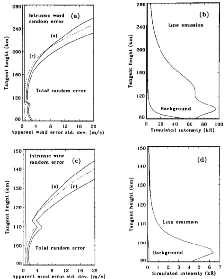
Figure 1 shows the apparent wind error standard de- viations and apparent emission rate profiles for column-

averaged quantities associated with typical day (Figures

la and lb respectively) and night observations (Figures

lc and ld) respectively) of the oxygen green line emis-

sion with WINDII. In the plots of the apparent emission

rate both the emission profile and the background ap- parent emission rate profile are shown. During the day- time the rapid increase in background apparent emis- sion rate at the lower altitudes due to Rayleigh scatter- ing is evident. In the plots of the apparent wind error

standard deviation the error associated with the shot

noise (designated s), the reading wind error (designated

r), the intrinsic random error, and the total random er-

ror are shown. In general, for both day and night the dominance of the error by the shot noise, when the ap- parent emission rate is high, is apparent. The reading wind error is significant at all heights but is more sig-

nificant when the apparent emission rate is low. The remaining contribution, the intrinsic wind random er-

ror, is due to the satellite and Earth rotation velocity

determination

(V/•s + rr•

2 = 0.1 m s-i), the zero

wind

determination

(rr• = 0.7 m s -1 for the mesosphere

and

0.5 m s -1 for the thermosphere),

and the calibration

phase

determination

(rr• = 0.3 m s-1). The intrinsic

wind random error is only significant in regions where the apparent emission rate is high.

3.3. Inverted Quantities

The reduction from line-of-sight integrated quantities to profiles in altitude is performed using three inversions

GAULT ET AL.' WINDII VALIDATION 10,411

280

Intrinsic

w•

200

.

160

240 200 160 120 80 o (b) Line emission •o 40 60 80 100 Simulated intensity (kR)

140

...

130

(d) n

Background

Figure 1. The apparent

wind

error

standard

deviations

and associated

emission

rate profiles

for

typical

(a and b) day and (c and d) night

conditions.

In the wind

error

standard

deviation

plots,

r indicates

the reading

wind error and s the error associated

with the shot noise.

of the form [e.g., Twomey,

1977;

Menke,

1984]

Xi -- (L•'S•-,•Li

+ '7iK/TKi)

-1 L•S•-,•yi (14)

where

xi Yi

Li

Syzz

is the solution estimate vector, is the data vector,

is the limb geometry transformation matrix of

the forward model yi: Lixi (see Equation 21

from Shepherd et al. [1993]),

is the diagonal data covariance matrix, is the damping constraint matrix, and

is the weighting parameter.

For the inversion,

Sy is calculated

without the contri-

bution of the intrinsic phase random error. Each con-

straint matrix is a variant of a differences matrix with

rows containing

[..., 0,-1, 1,0,...] or [..., 0,-1,2,-1,

0,...]. Relative

scaling

of constraint

matrix rows and

reduce the noise in the overall profile while retaining the smaller-scale features considered significant. While

work is continuing on refining the values used in the in-

version process, any future adjustments arc unlikely to

influence the overall results presented here. A detailed account of the inversion process will appear elsewhere.

Incorporating the damping term reduces the solution

random error variance estimates from

•r

2 - (L•-•Sy

L•-•')jj

(15)

to

-1

O'•.

i -- (L/TS•Li

q-

7Ki•'Ki)jj

(16)

These variances are then used to determine the final

wind random error standard deviation estimates. In the calculation of these variances only the random error

variance of the measurements (first term on the right-

hand side of equation

(11) are included

in the covariance

The induced error (composed of the discrctization

due to the finite bin size and the constraint bias), the

net signal noise (standard deviations

calculated

using

equation

15) and constrained

signal

noise

(standard

de-

•60 :/40 120 Constrained • 60 ,,,,...,,,.,.,.,... 0 I0 20 30 40 50 Doppler wind error std. dev. (m/s)

Vool.

cm.

rate

(photons/cma/s)

Simulated Doppler wind (m/s)

2oo

160

V0ol.

em.

rate

(photons/cm3/s)

,50

150

m.•

Volu.

Doppler wind error std. dev. (m/s) Simulated Doppler wind (m/s)

Figure 2. Typical error profiles for inverted winds and associated volume emission rate and

wind profiles

for (a and b) day and (c and d) night conditions.

and volume emission rate profiles typical of daytime

observations (see Figure 2b), are given in Figure

The corresponding nighttime profiles are shown in Fig-

ures 2c and 2d. Near the peak of the volume emission

rate profile the wind standard deviation is 6 m s -1 for

the daytime measurements

and 3 m s -1 for the night-

with the use of damping in the inversions and the min-

imal contribution of the induced error (apart from in

the region below the emission peak) is evident in these

figures.

The inverted profiles are calculated for each field of view and then combined to produce zonal and merid-

ional winds along the satellite track. These profiles are

then interpolated to produce the level 3 wind fields most

accessible to the scientific community. The errors pro- vided with these data are calculated using the appropri-

ate linear combination of the variances of the relevant

profiles. The potential difference between the initial

and the reduced standard deviations should be kept in mind when using WlNDII winds because the standard

deviations currently provided with the data are those

from equation (15) as opposed to those achieved with

the damping term, equation (16). The data are cal-

culated, however, using the damping term, so that the errors provided are larger than they should be given the method of calculation. In addition, the bin bias is not subtracted from the signal in the shot noise calcula-

tions. This results in an overestimation of the random

error variance of the same order as the reading error variance. These ambiguities will be resolved for data calculated using data processing software versions sub-

sequent to version 4.23. Since each solution profile is

determined independently from any other along the or- bit track, further noise filtering may be achieved, when desired by the data user, through carefully weighted combinations of neighboring profiles.

4. On-Orbit characterization

4.1. Horizontal Phase Corrections

The O1S zero reference

image was produced

by the

GAULT ET AL.' WlNDII VALIDATION 10,413

• --2

• --3

1 2 3 4 5 6

Column no.

Figure 3. Typical example of lateral phase varia-

tions: OiS, daytime bottom window of field of view

2 (FOV2), January 19, 1993. Averages for 20 rows of

pixels. Dashed line shows variations before the charac-

terization data base (CDB) adjustment, solid line after

adjustment. There are six columns of bins across each

field of view.

tion, the phase distribution was checked on orbit to the extent that it was possible.

It is not difficult to assess the lateral phase varia-

tions (along a row of pixels) by averaging many mea-

surements, because the lateral variations, on the scale of the field of view, are expected to be approximately random. This was done for several days at different

times in the mission by averaging the measurements for a whole day. Phase images were averaged separately for night and day apertures and for windows located in the upper and lower regions of the field of view. Mea-

surements made near the terminator were not used. An

example of the lateral variation is shown in Figure 3

(dashed line). It was generated by subtracting the row

average from each value in the row, and averaging 10

such rows. It represents the phase variations that are present after correction by the zero reference phase im-

age measured in the laboratory prior to launch. The lateral phase variations were found to be consistent for

the different times sampled.

These residual lateral phase variations were averaged for several days scattered through the mission and were then used to generate images to correct the column-to- column variations in the existing zero phase reference image without changing the average values for each row.

Figure 3 (solid line) shows data reprocessed using the

corrected reference data. Lateral variations still exist

in the data but are now about a third of the previous

ones. The corrections are not expected to change the wind values obtained for each row in the image but do

improve the statistics used in error estimates.

4.2. Filter Passbands

Interference filters can sometimes change their char-

acteristics over time, so it is useful to monitor their properties during the mission. On WINDII it has been

possible to study the passbands of the O1S and

filters on a regular basis using light from two of the

phase calibration sources. A technique has also been

developed to detect small changes in the tilt of the fil-

ters with respect to the optical axis. All the WlNDII

filters except for filter 5 were manufactured by Andover Corporation, who used a proprietary process to stabi-

lize their characteristics. Filter 5 (the broad-band OH

filter) was provided by Barr Associates.

The data used for the analysis come from the weekly major calibrations. In particular, absolute transmit- tance images of the filters taken with the night aperture

are obtained at the wavelengths

of the Kr (557.0 rim)

here are from a period beginning shortly after launch and ending in December 1•93. These data are cam-

160- _o 159- •: 158- o (i) 157- ._ 156

EEl

[3

[3 o o oo o

o oo

Days after launch

I I I [] [] [] [] [3 [] [] 0 [] oo [] [] (c) 176- E •75- 174- ---• 173- o • 172- _ Q_

Days offer launch (x10 *•)

125 ..• 124- E c • 123- • 122- ,

-

Days offer launch (x10 +2)

I I I I [] [] [] [] [] [] [] [] [] [] [] [] [] [] [] (d)

Days after launch (x10 +•)

Figure 4. Locations

of the normals

for the O1S and OlD filters as functions

of mission

time. (a

and b) Horizontal

and vertical

coordinates

for the OIS normal

(located

in FOV1). The prelaunch

values

are at day zero. (c and d) Same

for the OlD filter (in FOV2).

pared with similar transmittance images obtained be-

fore launch.

The transmittance images are circularly symmetric

and the center of the pattern marks the direction of the normal to the filter. A convenient way to study the

changes in the tilt of the filters is to plot the location of

the center of the transmission pattern as a function of time. For this purpose the centers of a selected number

of rings of constant transmittance were computed, and a weighted average of these centers was taken to be the estimated direction of the filter normal. Figure 4 shows

the horizontal and vertical locations of the estimated

centres for the OiS and O•D filters on the CCD for a

selected number of calibrations taken between launch

and the end of 1993. It can be seen from the plots that

there has been no significant drift in the tilts of the two filters since launch, although a slight shift of the order of 3 to 4 pixels in the horizontal direction toward the outer edge of FOV1 can be observed between the

ground (day zero) and flight positions for both filters.

The CDB has been adjusted for the effect of this small shift in the filter axis and no significant effect on the measurements is expected.

In examining the transmittance of the filters at the wavelengths of the calibration lamps, advantage was

taken of the inherent circular symmetry of the trans-

mittance images around the filter normal. The average

transmittance was computed for each image as a func-

tion of angular distance from the filter normal. Fig- ures 5a and 5c show typical plots of the averaged trans- mittance against angular distance from the estimated filter normals. The averaged transmittance at a selected number of incident angles was then plotted as a func-

tion of time. Figures 5b and 5d show variations in the

averaged transmittance at fixed angles from launch to

the end of 1993 for the O•S and O•D filters respectively.

The shift between the ground (day zero) and flight is

about -0.05 nm for both filters, and is likely due to a

temperature

difference.

Since

then the O•S filter has

shown no long-term drift exceeding +0.01 nm and the

OlD filter has apparently drifted back +0.03 nm, or 1%

of its bandwidth, during the time in orbit. These filters

can therefore be considered essentially stable.

Finally, although the transmittance of the two filters was studied using only the WINDII night aperture, it is reasonable to assume that similar results hold also for

the day aperture, which uses approximately 11% of the

area of the filter lying within the area used by the night aperture.

4.3. l•esponsivity

The tungsten halogen lamp is observed through each filter about once a week during the major calibrations

as a partial check on the instrument 's responsivity. Fig-

ure 6a shows the normalized response curves for filters 1 to 6. The response to the tungsten lamp has decreased

by 3 to 7% over 1100 days, with the most rapid change

near the beginning, and leveling off after day 800. This could be understood as a change of temperature of the tungsten lamp combined with darkening of the enve-

lope, affecting the shorter wavelengths (filters 1, 2 and

3) more than the longer ones. Other possibilities are radiation darkening of glass elements, changes in the in- tegrated filter transmittance, and changes in the CCD, in which case the instrument 's responsivity could be af- fected. As section 4.2 showed, filters 2 and 3 appear to

c- 7-

I I I i _

_

Angle to filter normal (deg)

40- 38-

36-

o []

o

Days offer launch

644 .642- o 640- o .638•

"• .636

Angle to filter normal (deg) Days offer launch

Figure 5. (a) Typical average transmittance as a function of angle from the O1S filter normal.

(b) The same

for the O•D filter. (c) Average

transmittance

60 from the O•S filter normal as a

function

of mission

time. The prelaunch

value is at day zero. (d) The same

for the O•D filter at

GAULT ET AL.' WINDII VALIDATION 10,415 1.02 1.00 0.98 0.96 0.94 0.92 0.90 , , • ß 4,5,6

f

(a)

....

"'

'-'•3

.-- t

Days after launch

1.02 1.00 0.98 0.96

0.94

0.90

(b)

• •A•

Days after launch

Figure 6. (a) CCD response

to the tungsten

calibra-

tion lamp as a function of mission time. Each curve

represents a different filter and is normalized to the ini-

tial point. The wavelengths for filters 1, 2, and 3 are,

respectively,

553 nm (background),

558 nm (O•S), and

630 nm (O•D). filters 4, 5, and 6 are the OH group,

plotted but are very similar •o the OH group. (b) Nor-

malized response of the lamp's photodiode monitor for

the same period. The wavelength is 540 nm. The dis-

crete levels are caused by coarse digitizaion. Data are not available for every calibration.

be very stable, so the effect is not likely due to them. Furthermore, Figure 6b shows that the change in signal from the tungsten lamp's monitor is about the same as

for filters 2 and 3. The monitor is a filtered photodiode

placed near the lamp with no intervening optics and

records the lamp output at 540 nm (bandwidth is equal

to 9 nm). Since the lamp is the one element common to

the measurements with the CCD and the monitor, it is reasonable to suppose that the observed changes have occurred in the lamp. Therefore no adjustments have

been made to the responsivity in the database. One curious feature of Figure 6a is that filter 1 seems out of place, being less affected by the changes than filters 2 or 3, which are at longer wavelengths.

4.4. Long-Term Phase Drift

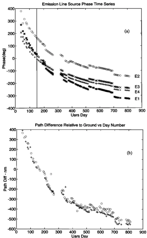
In addition to the expected small variations in phase due to thermal variations, a longer-term drift in the Michelson phase is observed which cannot be related to temperature. This drift was tracked using the weekly phase calibrations and is illustrated in Figure 7a for the

four emission line sources on WINDII, represented in

the figure as E1 (Kr 557.0 nm), E2 (Ne 630.5 nm), E3 (At 738.4 nm), and E4 (Ar 763.5 nm). Data are shown

for the first 810 days of flight, during which the phase changed by 450 ø to 6000 , depending on the wavelength.

The variation has the form of a relaxation process with

a timescale of about 225 days. The cause of the phase drift is not known but could be due to changes in the glass, the glue layers or dielectric coatings on the sur- faces, or a relaxation of the clamping pressure on the

interferometer. Gaps in the data correspond to times

when the UARS instruments were turned off. The sud-

den jumps in phase occur at resets, when the instru-

ment is powered on after having been turned off for

some reason, and the mirror alignment returns to a

slightly different setting. For each of these segments a new characterization database was constructed using

calibration data to account for the effect of these varia-

tions in phase. These changes have not had an adverse

effect on the Michelson 's ability to modulate emission

lines. The visibility of the laser source, measured during major calibrations, has remained above 0.9 throughout

the mission.

As mentioned in section 1, zero wind calibrations

were made on the ground prior to launch and are as-

sumed to be valid after launch. This assumption can- not be checked directly from the phase calibrations of

individual lines because of the possibility of changes

occurring in the interferometer during launch which

might cause phase wraparounds. This may, however,

be checked by considering the phase difference between calibrations at different wavelengths. This phase differ- ence is a slowly varying function of path difference and thus is much less susceptable to ambiguities than the phase of a single line.

The variations of phase differences (El-E2) and (E3-

E4) have been converted to changes in path difference

(assuming no dispersion) and are plotted in Figure 7b.

The agreement between the two curves is excellent and indicates that the assumption of no wraparound is cor- rect. The phase difference on orbit matches that on the

ground at day 151 for both cases. This date is indicated by the vertical line in Figure 7a. The ground phase dif-

ference does not match the phase difference on orbit at

day 0 because of the change in medium (air to vacuum)

in the interferometer gap between ground and orbit.

The results of this calculation indicate that the Michel-

son interferometer has been extremely stable with the

stresses of launch causing changes in the path difference of • 50 nm. Such changes are minimal and provide jus-

tification for the initial use of the ground calibration

data in orbit.

The gradual phase drift described here also implies

a drift in the zero reference because the phase calibra- tions and atmospheric measurements are made at dif-

ferent wavelengths.

In the case

of O•S the wavelength

difference is 0.7 nm, causing an effective shift of 9.5 m

s -• in the zero reference due to the observed increase

of 6000 of phase

(1.67 orders

of interference)

in the first

800 days of the mission. This effect is corrected in the

4OO 300 200 lOO -lOO -2oo- -3oo -

-4000

Emission Line Soarce Phase Time Series

i i 1 I i i o

+xx%

Path Difference Relative to Ground vs Day Number i i i i i i (b)

•

o

0

I

I

I

-60

100 200 300

900

o

-

_

o •' .•.

H++,•oO

_•½+

_•

o

-

Figure 7. Long-term phase variation. (a) Phase as a function of mission time for the four

calibration sources, E1 to E4. (b) Path difference relative to prelaunch values, calculated from

E1 to E2 and E3 to E4.

4.5. Limb Heights in the WINDII Images

The tangent limb altitudes for the image elements in each WINDII field of view were computed using UARS orbital information combined with a knowledge of the relative orientation of WINDII with respect to

the spacecraft. The approximate orientation was deter- mined before launch, but more precise on-orbit values

were obtained using weekly sequences of WINDII star images.

Because of the requirement for precise absolute limb heights, redundant methods were employed to evaluate the transformation matrix relating the spacecraft frame of reference to the WINDII instrument pointing frame for each field of view. The matrix elements were de- termined by referencing the absolute WINDII inertial