Designing and compiling functional Java for the Fresh Breeze architecture

Designing and Compiling Functional Java for the Fresh Breeze

Architecture

by

OF TECHNOLOGY

William J. Jacobs

JUL 2 0 2009

B.S. Computer Science and Engineerin

LIBRARIES

Massachusetts Institute of TechnologyI

Submitted to the Department of Electrical Engineering an Computer Science

in Partial Fulfillment of the Requirements for the Degree of

Master of Engineering in Electrical Engineering and Computer Science

at the Massachusetts Institute of Technolc gy

May 2009

ARCHIVES

©2009 William J. Jacobs. All rights reser ed.

The author hereby grants permission to reproduce and to disribute publicly paper

and electronic copies of this thesis document in whole or in part in any medium

now known or hereafter created.

Author_

.'

Department of Electrical Engineering and Compute Science

May 22, 2009

Certified by

.ack

Denlnis, Professor Emeritus

Thesis Supervisor

Accepted by

_____________

Arthur C. Smith

Professor of Electrical Engineering

Chairman, Department Committee on Graduate Theses

Designing and Compiling Functional Java for the Fresh Breeze

Architecture

by

William J. Jacobs

Submitted to the

Department of Electrical Engineering and Computer Science

May 22, 2009

In Partial Fulfillment of the Requirements for the Degree of

Master of Engineering in Electrical Engineering and Computer Science

Abstract

The Fresh Breeze architecture is a novel approach to computing that aims to support a high degree of parallelism. Rather than striving for heroic complexity in order to support exceptional single-thread performance, as in the Pentium and PowerPC processors, it focuses on using a medium level of complexity with a view to enabling exceptional parallelized performance. The design makes certain sacrifices with regard to capability in order to achieve a

lower degree of complexity. These design choices have significant implications for compiling for the architecture. In particular, Fresh Breeze uses immutable, fixed-size memory chunks rather than sequential, mutable memory to store data [1][2][3]. This work demonstrates Functional Java, a subset of the Java language that one can compile to Fresh Breeze machine code with relative ease, overcoming challenges pertaining to aliased arrays and objects. It also describes work on a compiler designed for the Fresh Breeze architecture and how the work overcomes various challenges in compiling Java bytecode to data flow graphs.

Thesis Supervisor: Jack Dennis Title: Professor Emeritus

1. Introduction

The Fresh Breeze processor design is in many ways a departure from conventional

design. It is designed to be highly parallelized, with simultaneous multithreading and hardware

support for spawning method calls to other processors or cores.

The Fresh Breeze system makes use of a memory model that is considerably different

from the standard model. In the standard memory model, memory is regarded as a linear array

of mutable memory locations. In the Fresh Breeze memory model, memory is allocated to a

thread of computation in 128-byte chunks, each of which is referenced by a unique UID or pointer. Each chunk may contain pointers to other chunks. Fresh Breeze memory chunks are

immutable in the sense that a thread may create a chunk and write data into it, but the chunk

becomes permanently fixed once shared with other threads. This behavior provides a guarantee

that the heap will never contain cyclic structures, ensuring that the heap forms a directed acyclic

graph. This enables efficient hardware garbage collection using reference counting [1][2][3].

The immutability of memory is well-suited to the functional programming paradigm,

which is concerned with functions that produce output values appropriate to a given set of inputs,

without altering the inputs to the function. In addition, immutable memory eliminates the concern of cache coherence by ensuring that any memory stored in a cache is always accurate.

In order to expedite the allocation of memory, the Fresh Breeze system relies on hardware

garbage collection that is implemented using reference counting. The usage of hardware-based memory allocation and deallocation greatly reduces the overhead typically associated with these operations. Furthermore, it solves problems associated with determining when a portion of memory that was available to multiple processors may be deallocated.

While the particular features of the Fresh Breeze model make the design well-suited to

scientific and other computation-intensive applications, they pose interesting challenges for a

compiler designed to target Fresh Breeze machine code. In particular, how can one ensure that the heap contains no reference cycles without unnecessarily burdening the programmer? The

aim of this paper is to describe the work involved in overcoming these challenges. This project

entails writing software that compiles Java bytecode to a data flow graph. In targeting the Java

programming language, the intent was to enable the programmer to use a familiar language,

while simultaneously enabling the compiler to produce efficient Fresh Breeze machine code. In addition, by using Java bytecode, we are able to leverage parsers and semantic analyzers that

already exist for the Java programming language in building the Fresh Breeze compiler.

The compilation of a program into Fresh Breeze machine code is a five-step process, as

illustrated in Figure 1. First, the Java compiler produces Java bytecode from Java code. This is

converted into an intermediate representation, which is subsequently compiled into a data flow graph. Optimization converts a data flow graph into an optimized data flow graph. Finally, this

L

LI

Java source code

Java compilation

Java becode

Conversion to IR

Intermediate

representation

Compilation

Data flow

graph

Optimization

Op

timized

data flow

raph

Code generation

Fresh Breeze

machine

code

Figure 1: The Compilation Process

The compilation process will operate on a single Java class as the basic unit of

compilation. Methods will be linked during the code generation phase by substituting the UID

(pointer) of the appropriate code object at each method call.

This project focuses on the design and programming of the conversion of Java bytecode

to an intermediate representation and subsequent compilation to data flow graphs. The objective

is to produce functional data flow graphs from Java classfiles with minimal restrictions on the allowable Java source code. Generation of machine code for the Fresh Breeze architecture is left

to future work.

The remainder of this thesis is organized into six sections. Section 2 describes a means of

overcoming the problem of aliasing in order to design a compiler that is compatible with the Fresh Breeze memory model. Section 3 describes an intermediate representation to which Java bytecode is compiled and the algorithms used to compile to it. In Section 4, this paper describes

the data flow graph representation to which the intermediate representation is compiled as well

as algorithms used in the compilation process. Section 5 details how the compiler checks

restrictions on the Java language pertaining to aliasing. In section 6, this treats the subject of

optimization, indicating how the compiler performs various optimizations. Finally, section 7 is

concerned with how this work may be extended and improved.

2. Aliasing

2.1. Functional Java

In the Fresh Breeze memory model, memory is immutable. This makes operations such

as changing an array's element or an object's field impossible, strictly speaking. Instead of

changing an object or array, a program must produce a copy of the object or array that differs

only in one of its fields or elements. This is consistent with the functional programming perspective, in which each method's purpose is to produce an output from a particular set of

inputs without altering any of the inputs. However, it poses a unique challenge when compiling

a non-functional language, such as Java.

In particular, aliasing presents a problem for a compiler designed to target Fresh Breeze

machine code. Aliasing refers to the ability to access a given portion of memory using multiple symbolic names in the source code. This is problematic when a particular object is altered. Because the object might be accessible from multiple variables, the compiler would need to ensure that regardless of the variable from which the object is accessed, the contents are the same.

In order to use the Fresh Breeze memory model correctly, one can impose restrictions on the permissible Java programs that ensure that aliasing cannot occur. Having eliminated aliasing, each computation can be expressed functionally; that is, in such a manner that each method produces a set of outputs from a given set of inputs without modifying any of the inputs. This successfully eliminates the need for mutable memory. Furthermore, since the computation is functional, method calls are necessarily independent, allowing the compiler to maximize the amount of parallelism in a given program.

In practice, to express each Java method as a functional computation, one can design the compiler to implicitly return modified copies of all of its arguments. Figure 2 contains an example of a code listing and the equivalent Fresh Breeze pseudocode.

Code:

class Foo {

int x;

public static void bar(Foo f)

f.x = 1;

public static void baz(Foo f) bar (f);

f.x++;

Fresh Breeze equivalent:

Foo bar (Foo f)

Foo f2 = alteredCopy(f, x - 1) Return f2 Foo baz(Foo f) Foo f2 = bar(f) Foo f3 = alteredCopy(f2, x - (f2.x + 1)) Return f3

Figure 2: Using Return Values to Implicitly Modify Arguments

This sort of compilation is capable of preserving Java semantics, so that the bar method

does what the programmer would expect. However, aliasing presents a problem for this sort of

approach. For example, consider the code and the Fresh Breeze equivalent presented in Figure 3.

Code:

class Foo {

int x;

class Bar {

Foo f;

public static void baz(Bar bl, Bar b2)

bl.f.x = 1;

Fresh Breeze Equivalent:

<Bar, Bar> baz(Bar bl, Bar b2) Foo f = bl.f

Foo f2 = alteredCopy(f, x - 1)

Bar b3 = alteredCopy(bl, f - f2)

Return <b3, b2>

Figure 3: Problem Arising From Aliasing

A problem arises if bl. f and b2. f are the same. In this case, the programmer would

expect both bl. f . x and b2. f . x to be changed to 1, in conformance with the standard Java

semantics. However, if one were to use the code in Figure 3, only bl . f. x would be changed;

b2 .f . x would be unaltered.

There are two fundamental approaches to the problem of aliasing. In one approach, the

program performs runtime checks to identify each instance of aliasing so that the compiler may

take the appropriate action. For example, one could rewrite the above baz function as

demonstrated in Figure 4:

<Foo, Foo> baz(Foo fl, Foo f2)

Bar b = fl.bar

Bar b2 = alteredCopy(b, x - 1)

Foo f3 = alteredCopy(fl, bar - b2) If f2.bar = b

f2 = alteredCopy(f2, bar - b2)

Return <f3, f2>

Figure 4: Runtime Correction ofAliasing

time in even some relatively common cases. For example, if a method is passed an array of 1,000 objects, every time one of the objects' fields is changed, the method would have to check

each of the other objects to see if they match the one that was changed.

Another approach is to place restrictions on what Java programs the compiler will accept.

This is the approach recommended here. By forbidding certain Java programs, one can ensure

that the problem of aliasing is avoided.

Having settled on this approach, the objective is to place as little restriction on the

programmer as possible. One might consider the simple solution of requiring objects to be

immutable, rejecting any program that modifies any object's field, as proposed in [5]. However, a less restrictive approach is possible.

One may describe object references using a directed graph. Each node in the graph

represents a single array or object. There is an edge from an array to each of its elements and

from an object to each of its fields. The solution to the problem of aliasing described here is a set

of compile-time checks designed to ensure that the graph of the references forms a forest. The

checks also guarantee that the parent of every object or array that is referenced in a method is known at compile time.

The restricted subset of Java is termed "Functional Java". The restrictions are as follows:

1. No reference argument to a method call may be a descendant of another argument or the same as another argument. For example, the following is disallowed:

void foo() {

Foo f = new Foo(); bar(f, f.bar);

2. A method may not return one of its reference arguments or one of their descendants. This rule forbids code such as the following:

Bar foo(Foo f) {

return f.bar;

3. No reference may be made a descendant of another reference, unless it is known to have no

parent. This prohibits behavior such as the following:

void foo(Foo f, Bar b) {

f.bar = b;

}

4. A reference variable may not be altered if the identity of its parent may depend on which branch is taken. The following, for example, is not permitted:

void foo(Foo fl, Foo f2) {

Bar b; if (baz()) b = fl.bar; else b = f2.bar; b.x = 1; }

5. A variable containing a reference descendant of an array may not be accessed or altered after a descendant of the array is altered, unless the variable was set after the alteration was performed. This forbids the following code, which would be problematic if the inputs a and b were the same:

void foo(Foo[] f, int a, int b) { Foo f2 = f[a];

Foo f3 = f[b]; f2.x = 1;

f3.x = 2;

}

6. A variable containing a reference descendant of an array may not be altered after the array is altered, unless the variable was set after the alteration was performed. The following is

forbidden by this rule, since a problem would arise if the inputs a and b were the same:

void foo(Foo[] f, int a, int b) { Foo f2 = f[a];

f[b] = new Foo();

f2.x = 2;

7. The == and != operators may not be used between any pair of references, unless at least one

of them is explicitly null. At any rate, because of the above restrictions, the result of such

an operation would be known at compile time (unless one of the operands is null), so the ==

or != was probably used in error.

Note that each of these conditions can be checked on a per-method basis. In particular, it

is guaranteed that if two classes can successfully be compiled separately, then they can be successfully compiled together.

In addition, static fields are required to be compile-time constants, as proposed in [5].

Otherwise, every method would have to accept the static fields as implicit arguments and

implicitly return the new values. At any rate, permitting variable static fields would not conform

to the paradigm of functional programming.

2.2. Implementing the Java API Using Functional Java

Much of the Java API requires a violation of one of the aliasing rules. For example, the

ArrayList class, which stores a dynamically sized array, has a method to add an element to the class. Figure 5 contains a simplified form of how it is implemented.

public void add(T element) {

this.array[pos] = element; pos++;

Figure 5: Implementation of ArrayLis t .add

This code is forbidden by rule 3, since element is made a descendant of this, both of

which are arguments to the method. In order to get around the restrictions, the programmer may use a Fresh Breeze library method of the form presented in Figure 6.

public class FBUtil {

public static native <E> E copy(E object);

}

Figure 6: The FBUtil . copy method

The method takes an object or array and returns a deep copy of it. Counter-intuitively,

the method takes no time at all. It simply returns its argument and causes the compiler to treat the returned object as if it were an unrelated object. This implementation is guaranteed to be

correct because in the Fresh Breeze memory model, memory is immutable.

The FBUtil.copy method provides a workaround for the ArrayList method shown

above. It may instead be implemented as presented in Figure 7:

public void add(T element) {

this.array[pos] = FBUtil.copy(element); pos++;

This alters the semantics of the ArrayList class. Now, instead of storing references to

objects, it would store copies of objects and would only permit retrieval of copies of its elements.

Another hitch pertaining to the standard Java library arises with regard to the equals

function. For example, say a programmer were to implement a class FBHashSet that is similar

to the Java HashSet class, except that it uses the copying semantics suggested above. Then, say

the programmer uses the class as shown in Figure 8:

boolean foo ()

Foo f = new Foo();

FBHashSet<Foo> fs = new FBHashSet<Foo>(); hs.add(f);

return hs.contains(f);

Figure 8: Using FBHashSet

This method would not return true as expected, unless the Foo class correctly overrides

the Obj ect. equals and Obj ect. hashCode methods. This is because the method adds a copy

of f rather than a direct reference to f to the FBHashSet.

Some of the instance methods in the Java library are specified to return the objects on which they are called. Such methods are a violation of the second aliasing rule. One example of

public class StringBuilder {

public StringBuilder append(CharSequence s) { return this;

Figure 9: Aliasing in the StringBuilder Class

Methods of the StringBuilder class are special from the perspective of the Java

compiler, since expressions such as str + "something" are typically compiled by creating a

temporary StringBuilder object and calling one of the append methods. In order to permit

compiling such expressions, the compiler treats the return values of a hardcoded set of library

methods that return this differently.

It is not immediately obvious how burdensome the restrictions imposed by Functional

Java are on the programmer. To get a sense of this, and to enable users of the Fresh Breeze

system to program using the standard Java API, it was useful to reimplement much of the Java API in order to satisfy these restrictions.

Experience suggests that for some tasks, it is difficult to conform to the restrictions. In

particular, it is difficult to work with chains of objects that may be of arbitrary length, as in linked lists and binary search trees. The implementation of a red-black tree and a hash table uses

integers to serve as pointers to nodes in the red-black tree and nodes in the linked lists in the hash

table, which took difficulty to maintain correctly. However, for most tasks, it took little effort to keep from violating the aliasing restrictions, particularly with the assistance of a compiler that

provided the file and line number of any such violations.

following the aliasing restrictions, the primary target of the Fresh Breeze system is computation-intensive scientific applications. For these applications, which often make less use of high-level

constructs than other programs, it seems likely that following the aliasing rules would be easier.

In general, while the restrictions may be limiting to people used to working with user-end PC's,

who are often concerned with programs that require careful design and make use of Java's more advanced features, it is probably not very limiting to those writing scientific programs, who tend

to rely on arrays and matrices for algorithms such as the Fast Fourier Transform and the

Cholesky algorithm.

2.3. A Possible Extension to Functional Java

One possible extension to Functional Java would be to behave differently when dealing

with immutable objects, which are understood to be objects consisting only of final, immutable

fields whose constructors do nothing but set these fields. This would allow relaxation of the

restrictions in certain cases. For example, one could allow immutable objects to be made children of multiple objects or arrays. Such an extension would cause Functional Java to be

strictly less restrictive.

However, there is at least one reason why such an extension might not be desirable.

Specifically, it is difficult to know the intent of the programmer when writing a class. A programmer might create a class that is initially very simple, which might by accident be immutable. The programmer might start using this class in several places with the intent of making the class mutable later on. He might inadvertently write code that would violate the aliasing restrictions if the class were mutable. When the programmer changes the class to be

mutable, numerous aliasing restrictions would appear.

At any rate, this possible extension affects the convenience of the language but not its power. Any case where one could refer to an immutable object with the extension but not without it can be corrected by a call to the FBUtil. copy method described in section 2.2.

2.4. Related Work

Previous work pertaining to aliasing has largely been focused on alias analysis within common languages such as C that permit aliasing. Such analysis is intended to improve optimization rather than eliminate aliasing [4]. This is understandable, since the memory model in use on conventional processors allows arbitrary mutation of data stored in memory.

Some functional languages allow the programmer to indicate occasions in which aliasing cannot occur. One way of doing so is uniqueness typing, which permits each object that the programmer declares to be linear to appear only once on the right-hind side of an assignment. Similarly, in a linear type system, once a value is cast to a linear form, the value can only be used once in the right-hand side of an assignment [7]. Like the work in this paper, such systems involve using compile-time checks to ensure that aliasing does not occur. However, these alternative systems are generally aimed at limiting aliasing rather than eliminating it outright. Furthermore, by comparison with the aliasing rules presented in section 2.1, they are particularly restrictive.

3. Compiling to Intermediate Representation

When compiling a program from Java bytecode to a data flow graph (DFG)

representation, it is helpful to first convert the bytecode into an intermediate representation. The

primary motivation for using this intermediate step is the fact that Java bytecode expresses some

variables implicitly as positions on a stack, but it is more useful to refer to each variable explicitly. In addition, such a conversion enables the compiler to more easily keep track of the

datatype of each variable that it is considering, which may enable certain optimizations at a later time.

The intermediate representation is based on the representation used in [5]. It consists of sequences of statements. Each particular type of statement is represented as a subclass of the

abstract IrStatement class. Control flow is represented by IrCondBranch statements, which

perform conditional branches, and IrUncondBranch statements, which perform unconditional

branches. Statements typically operate on operands, which are represented as instances of

IrOperand. Each IrOperand is either a fixed constant, using the IrConstant subclass, or a

variable reference, using the IrReference subclass. IrOperand objects store the type of the

operand. At this stage in compilation, the compiler does not determine whether a reference operand is an object or an array; this determination is deferred to a later time. The relevant class hierarchy appears in Figure 10.

IrStatement IrBranch IrCondBranch IrUncondBranch IrOperand IrReference IrConstant

Figure 10: Partial Class Hierarchy for the Intermediate Representation

In order to convert the implicit information about variables on the stack and in the local

variable array to explicit variable references, the compiler uses a StackAndLocals class. For

each stack or local variable position, the StackAndLocals class keeps a map from each

datatype to an IrReference. Each such IrReference is used to hold any value of its

respective type that is stored in its respective position. In addition, the class keeps track of the

datatype that is stored in each stack and local position at the current point in compilation. Using

this construction, each push of a value X onto a stack or store operation of a value X into a local

variable can be compiled as an assignment of the value X to the appropriate variable.

Using the StackAndLocals class, it is generally easy to compile bytecode to an

intermediate representation. Java bytecodes represent relatively simple operations, such as

pushing the value 2 onto the stack or converting the top item on the stack from an integer to a floating point value. For most bytecodes, the compiler can pop any operands it needs from the

stack, perform the desired operation on them, store the result in a temporary variable, and push

the variable onto the stack, using the StackAndLocals class to take care of the details of

pushing and popping.

One challenge in producing the intermediate representation is determining the type of elements stored in each array on which an array get or set operation is performed. This type

includes the number of dimensions in the array and the type of elements stored in the array.

Each array get or set operation is required to store the exact type of the array in question. Doing

so gives the compiler the flexibility to store arrays and objects differently, to store multidimensional arrays as single-dimensional arrays if desired, to store arrays containing

different types of elements differently, and to perform other optimizations.

It is not trivial to determine the type of each array because the aastore and aaload bytecodes, which set and get an array element respectively, only indicate that some sort of

reference is being stored in or retrieved from an array. The compiler does not immediately know whether the reference is another array or an object. Furthermore, a given variable may be one

type of array in one location in the bytecode and another type of array in another location.

However, if the compiler observes the entire body of the method, there will necessarily be

enough information to make the desired determinations.

Because the compiler may need to look at a method's entire body to determine array

types, it defers the computation until it has compiled the whole method to its intermediate

representation. Once a method is compiled, to compute the types of the arrays, the compiler relies on fixed-point computation. The aim of the computation is to determine the type of array

stored in each array variable at the beginning of each basic block of the program. Here, a "basic block" is understood to be a maximal sequence of statements to which only the first can be

jumped.

For each basic block, the algorithm first compute a sequence of "generated" mappings

from variables to array types. It does this by maintaining a map from IrReferences to array

some array variable referred to in the statement, it adds an entry to the map, replacing any existing entry for the variable. For example, it would know the type of any array that is the

return value of a method call or is a field it is retrieving from an object.

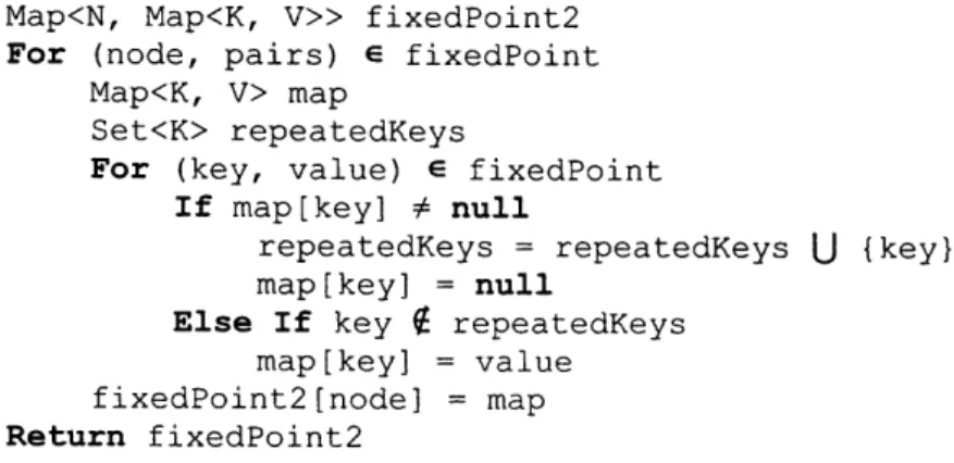
Once the algorithm has computed this information, it makes use of a fixed-point

algorithm. The algorithm is a special case of the fixed-point algorithm that is commonly used. The algorithm appears in Figure 11.

Map<N, Map<K, V>> doFixedPointMapUnion(Map<N, Map<K, V>> initialValues,

Map<N, Map<K, V>> generated, Map<N, Set<K>> killed, Map<N, Set<N>> successors) Map<N, Set<V>> allValues

For map e initialValues

For (key, value) 6 map

allValues[key] = allValues[key] U {value}

For map E generated

For (key, value) 6 map

allValues[key] = allValues[key] U {value}

Map<N, Set<Pair<K, V>>> initialValues2 For (node, map) 6 initialValues

For (key, value) 6 map

initialValues2[node] = initialValues2[node] U {(key, value)}

Map<N, Set<Pair<K, V>>> generated2 Map<N, Set<Pair<K, V>>> killed2 For (node, map) e generated

For (key, value) 6 map

generated2[node] = generated2[node] U { (key, value) }

For value2 6 allValues[key]

killed2[node] = killed2[node] U {(key, value2)}

For (node, keys) 6 killed

For key 6 values

For value e allValues[key]

killed2[node] = killed2[node] U {(key, value)} Map<N, Set<K, V>> fixedPoint

fixedPoint = doFixedPointUnion(initialValues2, generated2, killed2, successors)

Map<N, Map<K, V>> fixedPoint2 For (node, pairs) 6 fixedPoint

Map<K, V> map

Set<K> repeatedKeys

For (key, value) 6 fixedPoint

If map[key] # null

repeatedKeys = repeatedKeys U {key} map[key] = null

Else If key E repeatedKeys map[key] = value

fixedPoint2[node] = map

Return fixedPoint2

Figure 11: An Algorithm for Fixed-Point Computation With Maps

Map<N, Set<V>> doFixedPointUnion(Map<N, Set<V>> initialValues, Map<N, Set<V>> generated, Map<N, Set<V>> killed, Map<N, Set<N>> successors)

Map<N, Set<N>> predecessors For (node, nodes) E successors

For node2 e nodes

predecessors[node2] = predecessors[node2] U {node}

Map<N, Set<N>> in Map<N, Set<N>> out

Set<N> changed

For (node, succ) E successors If initialValues[node] = null

changed = changed U {node} out[node] = generated[node] Else

in[node] = initialValues[node]

out[node] = in[node] U generated[node] - killed[node]

While changed # {

N node = Any element in changed

changed = changed - {node}

Set<V> newIn

For node e predecessors[node]

newIn = newIn U out[node] If newIn # in[node]

in[node] = newIn

out[node] = newIn U generated[node] - killed[node]

For node2 E successors[node] changed = changed U {node2} Return in

Figure 12: Fixed-Point Algorithm

The method doFixedPointUnion is a standard and well-studied algorithm. In practice,

implementations of the algorithm operate by storing sets of values as bit vectors, which enables them to perform the union and difference operations efficiently.

The idea of the doFixedPointMapUnion algorithm is to make use of the standard

fixed-point algorithm by representing mappings as sets of key-value pairs. The algorithm

converts the generated and killed mappings into generated and killed key-value pairs, passes these pairs to the ordinary fixed-point algorithm, and converts the results into the appropriate

maps. Note that in the case of determining array types, there are no killed keys, while the

initialValues map consists of a mapping from the first basic block to the types of each array

argument to the method.

In fact, this algorithm by itself is insufficient to determine every array type. Sometimes,

it is necessary to know one variable's array type before another variable's array type can be discovered. In reality, the compiler runs the algorithm several times, each time using

information from the previous run to expand the set of generated mappings, until the algorithm

produces the same results twice in a row. Once the compiler has determined the type of each relevant array variable at the beginning of each basic block, it is a relatively simple matter to

determine the type of each relevant array variable within each basic block.

Once the program has compiled each method to its intermediate representation, it inline the "access" methods. Access methods are methods the compiler generates that are designed to

assist in information hiding. Access methods are of three types: retrieving a private field, setting

a private field, and calling a private method. Nested classes that have access to these private

fields and methods use such access methods rather than directly accessing the fields and

methods. Inlining these methods enables the compiler to correctly identify violations of the aliasing rules presented in section 2.1 when compiling the intermediate representation to data

flow graphs.

After producing a sequence of statements for the intermediate representation, the compiler creates a corresponding control flow graph. The control flow graph is essentially the same as the sequence of statements, except that it includes nodes to represent the basic blocks and edges to represent conditional or unconditional jumps. Creating the control flow graph

makes it easier to compile the intermediate representation into a data flow graph.

4. Compiling to Data Flow Graphs

The compiler represents each method in a program as a data flow graph, using a representation inspired by [5] and [6]. Data flow graphs are contrasted with control flow graphs

(CFGs), which are a more common representation. Control flow graphs represent a program as a graph of basic blocks, each consisting of a sequence of statements. Each node has edges to the

nodes to which it might subsequently branch. By comparison, a data flow graph represents a

program as a directed, acyclic graph containing nodes representing various operations. Each

node's inputs are indicated by the incoming edges.

Data flow graphs are particularly appropriate for functional programming. Because no

statement has any side effects, the predecessor-successor relationships represented in a data flow

graph are a natural representation of the order in which computations must be performed. A data

flow graph represents control flow implicitly using special constructs like conditional graphs. To get a sense for how data flow graphs can represent a method, some examples ought to

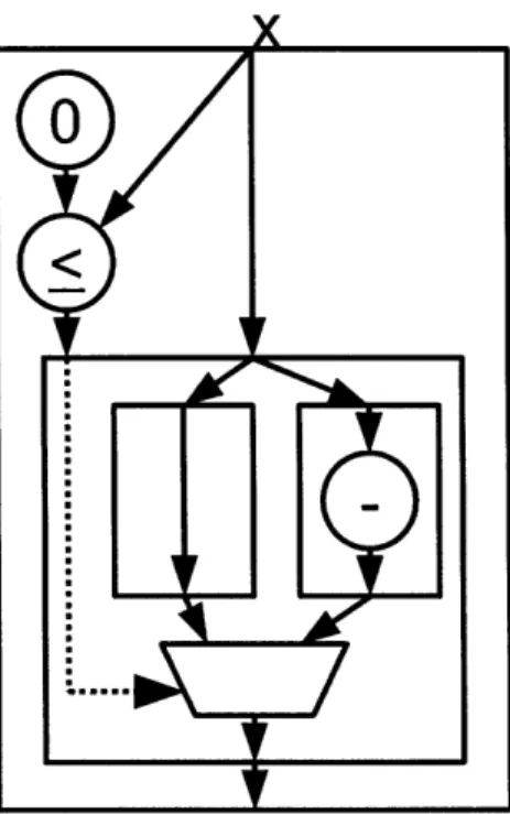
be of assistance. Figure 13 provides a data flow graph representation of the absolute value method.

Code:

int abs (int x) {

if (0 <= x)

return x; else

return -x;

}

Data Flow Graph:

Figure 13: Data Flow Graph Representation of the Absolute Value Function

The data flow graph for the absolute value method begins by comparing the input to 0. The result of this computation is provided as an input to a conditional graph, which is a subgraph of the method. Depending on the result of the comparison, the conditional graph executes either its left subgraph or its right subgraph. In the former case, it returns the input to the method; in

the latter case, it negates the input and returns the result.

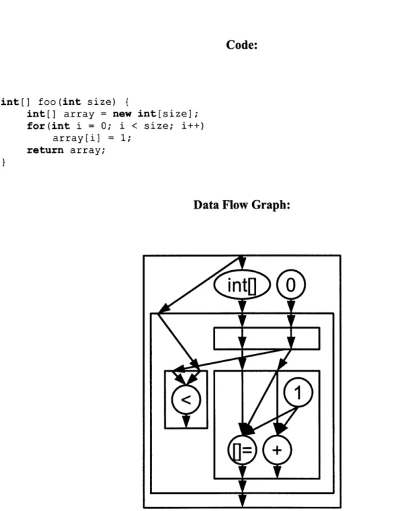
As another example, consider the data flow graph in Figure 14 for the method foo, which creates a new array and initializes it to all ones.

Code:

int[] foo(int size) {

int[] array = new int[size]; for(int i = 0; i < size; i++)

array[i] = 1;

return array;

}

Data Flow Graph:

In this example, the input is passed to a node that creates a new integer array of that

length. Then, the result is passed to a loop graph. The loop graph consists of an initialization subgraph, a test subgraph, and a body subgraph. The initialization subgraph, which is the one on

top, computes the initial values for the loop-dependent variables, array and i in this case. The

test subgraph, which is on the left, checks whether i is less than size; if so, the method perform

another iteration of the loop. The body of the loop, which is on the bottom-right, takes the values

stored in the loop-dependent variables array and i at the beginning of one iteration and

computes the values that are stored in these variables at the end of the iteration. The addition node in the body increments the loop counter. The node labeled []= takes as inputs an array, an

index, and a value and outputs an array that is the same as the input array, but with the element of

the given index set to the given value. The final value of array is used for the return value of

the method.

Each data flow graph and subgraph contains a source node and a sink node. A source node accepts no inputs and outputs the inputs to the corresponding graph. Likewise, a sink node

has no outputs, and its inputs are used as the outputs to the corresponding graph. To make data flow graphs easier to visualize, the source nodes and sink nodes are not shown in the diagrams for DFGs.

Although producing a correct data flow representation of a program is relatively difficult,

the usage of data flow graphs generally simplifies the process of transforming and optimizing a given program. In control flow graphs, one is often concerned with keeping track of what is stored in each variable at any given time. Data flow graphs, by contrast, eliminate the need for such bookkeeping by abstracting the locations of intermediate results of the computation.

Determining where to store each of the intermediate values is left to the code generator, which is responsible for converting the data flow graphs to machine code.

4.2. Identifying Loops

The process of compiling the intermediate representation to its data flow graph representation is a relatively difficult one. To begin with, the compiler converts the sequence of statements in the intermediate representation into a control flow graph. Then, it order the nodes in the control flow graph into an array so that each loop occupies a contiguous range of elements in the array. Doing so makes it easier when it eventually compiles the loops.

As it turns out, it is not trivial to identify the loops in a particular program. A simple definition of a loop is "a maximal set of nodes for which there is a path from each node to every other node." However, this definition is insufficient for the purposes of the compiler. For example, consider the loop shown in Figure 15.

for(int i = 0; i < n; i++) { for(int j = 0; j < n; j++)

if (i + j == 5)

return j; }

Figure 15: Nested Loops

Using the simple definition of a loop, the node containing the statement return j is not contained in the inner loop. In this case, since the statement can be reached from the inner loop, one would say that it is contained in the inner loop. This suggests a refined definition of a loop:

"A loop is a maximal set of nodes S for which there is a path from each node to every other node, along with the set of nodes T that cannot exit the loop without reaching a return statement."

In fact, even this definition is insufficient for the purposes of the compiler. Consider the code shown in Figure 16.

int i; for(int i = 0; i < n; i++) if (i == 5) { i = 3; break; i += 2;

Figure 16: Interruption of Control Flow in a Loop

Here, the statement i = _{3 ought to be contained in the first loop, but according to the}

above definition, it is not in any loop. Cases like this pose an additional problem for compilation.

To address these problems, when the compiler orders the statements, it first orders them

so that all loops occupy a contiguous range of nodes, if one excludes "dead end" nodes and "break" nodes. "Dead end" nodes are defined to be nodes that cannot exit the loops in which

they appear without reaching a return statement, while "break" nodes are defined to be nodes that

can be included in a loop but cannot reach the beginning of the loop. Then, the compiler "fixes" the dead end and break nodes so that they are in the correct positions.

The orderBeforeFix method, in which the compiler establishes a partially correct ordering, appears in the appendix. The algorithm goes through the nodes in a particular order, so that the first node in each nested loop is visited before any other node in the nested loop and each

node that is not in a nested loop is visited before any of its successors. For each node, it determines whether the node is in a loop. If so, it computes the nodes in that loop, stores them in a group, and adds the group to a set of groups. Otherwise, it stores only the node itself in a group and adds that group to the set. After grouping the nodes, it orders the groups topologically, putting each group before all of its successors. Finally, it produces an ordering of nodes by going through the groups in order, recursively ordering each group and adding the nodes in order to the output list.

To identify the nodes contained in a loop, the compiler first locates every subsequent node that can reach the first node in the loop using dynamic programming. It checks each node that is a successor of some loop node to see whether it is a dead end. It adds such dead end nodes to the deadEnds set, and it adds each such node along with every node it can reach to the set of loop nodes. Then, the compiler remove each node with a predecessor that is not in the loop from the set of loop nodes.

Having roughly ordered the nodes, the compiler needs to fix the locations of break nodes and dead end nodes. It begins by computing the successor of each loop; that is, the node which is executed immediately after each loop in "normal" control flow. It uses the computeLoopSuccessors algorithm presented in the appendix.

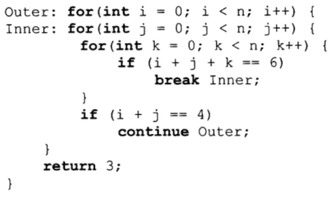
Computing the successor of each loop is relatively complicated because there are cases in which one is constrained to make a dead end node the successor of a loop. For example,

Outer: for(int i = 0; i < n; i++) { Inner: for(int j = 0; j < n; j++) { for(int k = 0; k < n; k++) if (i + j + k == 6) break Inner; if (i + j == 4) continue Outer; return 3;

Figure 17: Interruption of Control Flow in Nested Loops

In this case, the compiler needs to ensure that the successor of the second for loop is the

statement return 3 rather than the statement i++. More generally, it needs to ensure that dead

end nodes with predecessors in multiple loops are the successor of some loop.

The algorithm operates by identifying all dead end nodes that have predecessors in

multiple loops. For each, it identifies the children of the lowest common ancestor of the loops that contain the predecessors of the dead end node. For instance, in the above code, the

statement return 3 is a dead end node that has predecessors in multiple loops, namely the

inner two loops. The lowest common ancestor of these loops is the second loop, and the only

child of this is the innermost loop. For each loop, the algorithm also identifies the set of nodes within the loop have a predecessor in an inner loop.

Next, the compiler orders the loops so that each loop appears before the loop in which it is enclosed, and it goes through the loops in order. The current loop will have a set of nodes X containing zero, one, or two nodes that have a predecessor in an inner loop, if one excludes break nodes. Each node in X will be either the successor of the loop or the node to which a continue statement from an inner loop jumps. There is also a set of nodes Y consisting of dead end nodes

that need to be the successor of the loop or one of its ancestors. If X has no nodes, take a node

from Y and make it the successor of the loop. If X has two nodes, make the earlier of the two the successor of the loop. If X has one node, the algorithm needs to determine whether the node

may be the target of a continue statement from an inner loop. This is the case if every path from the start of the loop back to the start passes through the node. If the node may be the target of a

continue statement, make an element of Y the successor of the loop; otherwise, make the node in X the successor.

Having computed the successor of each loop, the algorithm can proceed to fix the

ordering of the nodes. The fixOrder method and the order method that makes use of it

appear in the appendix.

4.3. Identifying If Statements

Another challenge related to the inability to directly express control flow statements in

data flow graphs pertains to if statements. In the absence of explicit branching, the compiler

expresses conditional statements in data flow graphs as DfgConditionalGraphs. Each

DfgConditionalGraph accepts a special boolean input edge. If the input evaluates to true, the

program executes the left subgraph of the DfgConditionalGraph; otherwise, it executes the

right subgraph. The outputs of the subgraphs flow into DfgMergeNodes, each of which has one

input per subgraph and one output. Each DfgMergeNode selects as its output the input that

corresponds to the subgraph that was executed.

In order to be able to compile if statements, the first goal is to locate the beginning and end of each if statement. The beginning of an if statement is understood to refer to the first CFG

node containing a conditional branch for the if statement, while the end of an if statement refers

to the node where a program continues execution after executing the if statement. To identify the

beginning nodes, the compiler goes through the nodes in order, so that it visits each node before any of its successors (ignoring the edges to the beginning of each loop). Whenever it finds the

beginning of an if statement, it computes its end and the beginning nodes of each of its branches.

Then, it recursively identifies if statements that are contained in each of the if statement's

branches. The algorithm continues searching for the beginnings of if statements at the ending node of the if statement.

To compute the end of each if statement given its beginning, one may use the algorithm

in Figure 18:

void findReachableNodes(Node start, Node end, Loop loop, Set<Node> &reachable, Map<Node, Loop> enclosingLoops, Boolean isFirstCall)

If start e reachable Return

reachable = reachable U {start} If start = end

Return

Node enclosingLoop = enclosingLoops[start] Node loopStart

If enclosingLoop # null

loopStart = enclosingLoop.start Else

loopStart = null

If (start = loopStart and Not isFirstCall) or enclosingLoop # loop If enclosingLoop.successor # null

findReachableNodes(enclosingLoop.successor, end, loop, reachable, enclosingLoops, false)

Else

For succ in start.successors If succ # loopStart

Loop loop2 = enclosingLoops[succ]

If loop2 = loop or (loop2 # null and loop2.parent = loop) findReachableNodes(succ, end, loop, reachable,

Node findIfStatementEnd(Node start, Node except, Map<Node, Loop> enclosingLoops, Map<Node, Set<Loop>> loopSuccessors, Map<Node, Int>

nodeIndices)

Set<Node> reachable

findReachableNodes(start, except, enclosingLoops[start], reachable, enclosingLoops, true)

reachable = reachable - {except}

Loop enclosingLoop = enclosingLoops[start] Node loopStart

If enclosingLoop # null

loopStart = enclosingLoop.start Else

loopStart = null

Map<Node, Int> unreachablePreds unreachablePreds[start] = 0

PriorityQueue<Node> queue sorted by predicate(nodel, node2) If nodel # loopStart and node2 = loopStart

Return nodel

Else If nodel = loopStart and node2 # loopStart Return node2

Else If unreachablePreds[nodel] = 0 and unreachablePreds[node2] > 0 Return nodel

Else If unreachablePreds[nodel] > 0 and unreachablePreds[node2] = 0 Return node2

Else If nodeIndices[nodel] < nodeIndices[node2] Return nodel

Else If nodeIndices[nodel] > nodeIndices[node2] Return node2

Else

Return null

queue = {start}

Set<Node> visited

Boolean first = true

While Iqueuel > 1 or first

first = false

Node node = First element in queue

queue = queue - {node}

visited = visited U {node} Set<Node> ss If enclosingLoops[node] = enclosingLoop ss = node.successors Else ss = {enclosingLoops[node].successor} For succ E ss If succ = except Continue

If enclosingLoops[succ] = enclosingLoop or (enclosingLoops[succ] # null and enclosingLoops[succ].parent = enclosingLoop)

Int count = unreachedPreds[succ]

If count = null

//Compute the number of unreachable predecessors

For loop e loopSuccessors[succ] If loop.parent = enclosingLoop

preds = preds U {loop.start} count = 0

For pred e preds

If pred e reachable and pred 0 visited and pred # succ

count = count + 1 unreachablePreds[succ] = count queue = queue U Isucc}

Else

unreachablePreds[succ] = count - 1 If Iqueuel > 0

Node node = First element in queue

If (enclosingLoops[node] = enclosingLoop or (enclosingLoops[node] # null and enclosingLoops[node].parent = enclosingLoop)) and (enclosingLoop =

null or node # loopStart) Return node

Else

Return null Else

Return null

Node findIfStatementEnd(Node start, Map<Node, Loop> enclosingLoops, Map<Node, Set<Loop>> loopSuccessors, Map<Node, Int> nodeIndices)

Return findIfStatementEnd(start, null, enclosingLoops, loopSuccessors,

nodeIndices)

Figure 18: Finding the End of an If Statement

Note that in the pseudocode representation of this algorithm, as in all pseudocode presented in this paper, an ampersand in front of a parameter indicates that changes to the parameter are reflected in the calling method; otherwise, changes are not reflected in the caller.

The general approach of the algorithm is to maintain a priority queue of nodes. It sorts the nodes by whether each of their predecessors that is reachable from the starting node has been

visited yet, then by their indices in the previously established node ordering. At each iteration, it

extracts an element from the queue and add its successors to the queue. It continues until the queue has one or zero elements left. The remaining element, if any, is typically the end of the if

statement.

Once the compiler has located the end of an if statement, it identifies its branches. Each if-else statement will have two branches, which begin at two particular nodes, while each if statement will have one branch, beginning at a particular node. For the sake of consistency, the compiler considers if statements without else branches to have two branches: one for the contents of the if statement and one at the end of the if statement.

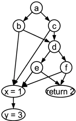
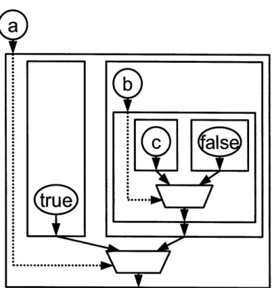
Often, the branches of the if statement are simply the successors of the beginning node of the if statement. However, the ternary ? : operator and the short circuiting behavior of the & & and I I operators pose a particular difficulty in identifying the branches, because in general, an if statement's condition may consist of multiple nodes. Intuitively, the branches are the earliest disjoint groups of nodes beginning with "choke points" in the graph through which a program must pass to go from the beginning of the if statement to the end. The example in Figure 19 illustrates one occasion when it is difficult to programatically identify the branches of an if statement. Code: if ((a ? b : c) II (d ? e : f)) x = 1; else return 2; y = 3;

Data Flow Graph:

Figure 19: Data Flow Graph Representation of a Complex Condition

To compute the branches of an if statement, the compiler uses the findBranches

algorithm shown in Figure 20.

void findBreakNodes(Node start, Node end, Set<Node> visited, Set<Node> &breakNodes, Map<Node, Loop> enclosingLoops, Map<Node, Loop> loopStarts)

If start = end or start E visited Return

visited = visited U {start) For succ 6 start.successors

If succ = end

Continue

If succ.successors = {}

breakNodes = breakNodes U {succ}

Else If enclosingLoops[succ] = enlcosingLoops[start]

findBreakNodes(succ, end, visited, breakNodes, enclosingLoops, loopStarts)

Else

If loop # null and loop.successor # null and loop.parent = enclosingLoops[start]

findBreakNodes(loop.successor, end, visited, breakNodes, enclosingLoops, loopStarts)

breakNodes = breakNodes U {succ}

Node latestNodeBeforeBranches(Node start, Node end, Set<Node> &breakNodes, Map<Node, Int> nodeIndices, Map<Node, Loop> enclosingLoops)

Set<Node> reachable

findReachableNodes(start, end, enclosingLoops[start], reachable, enclosingLoops, true)

PriorityQueue<Node> reachableSorted sorted by predicate(nodel, node2) If nodeIndices[nodel] < nodeIndices[node2]

Return nodel

Else If nodeIndices[nodel] > nodeIndices[node2] Return node2

Else

Return null

reachableSorted = reachable Map<Node, Set<Node>> reachable2 For node e reachableSorted

If node.nextIfFalse # null List<Set<Node>> reachable3 For succ E node.successors

If succ E reachable and succ 0 breakNodes Set<Node> reachable4 = reachable2[succ]

If reachable4 = null

reachable4 = {}

findReachableNodes(next, end, enclosingLoops[node], reachable4, enclosingLoops, true)

reachable2[succ] = reachable4 Add reachable4 to reachable3 Else

Add {succ} to reachable3

If (reachable[0] n reachable[l]) - {except} = {}

Return node Return start

Pair<Node> findBranches(Node start, Node end, Map<Node, Loop> enclosingLoops, Map<Node, Int> nodeIndices, Map<Node, Loop> loopStarts)

Set<Node> breakNodes

findBreakNodes(start, end, {}, breakNodes, enclosingLoops, loopStarts) Node latest = latestNodeBeforeBranches(start, end, breakNodes,

nodeIndices, enclosingLoops)

Node enlosingLoop = enclosingLoop[start] If enclosingLoops[latest] # enclosingLoop

Return (latest, null)

Else If end # null and ((latest.next = end and latest.nextIfFalse 4 breakNodes) or (latest.nextIfFalse = end and latest.next f breakNodes))

Return (end, findIfStatementEnd(start, end)) Else

If enclosingLoop # null and enclosingLoop.start = branchl

branchl = null

Node branch2 = latest.nextIfFalse

If enclosingLoop # null and enclosingLoop.start = branch2

branch2 = null

If branchl = null

branchl = branch2 branch2 = null

Return (branchl, branch2)

IfStatementInfo computeIfStatement(Node start) Node end = findIfStatementEnd(start)

Pair<Node> branches = findBranches(start, end) If branches.second = null end = null IfStatementInfo info info.start = start info.end = end info.branchl = branches.first info.branch2 = branches.second Return info

Figure 20: Pseudocode For findBranches

The general strategy of this algorithm is to identify the latest node that is before either of the branches. Such a node is usually the earliest node with two successors for which the set of nodes reachable from each of its successors is disjoint. In addition to computing the branches of an if statement, the computeIfStatement method also corrects for certain cases in which the end of the if statement was initially computed incorrectly.

4.4. Compiling Data Flow Graphs

To compile a method to a data flow graph, the compiler make use the Frame class. The intent of the class is to keep track of the edges that contain the values of each of the variables.

Frame stores a reference to a parent Frame, which may be null. Whenever the compiler needs

to obtain the value of a variable in a frame, it sees whether the frame has an edge for that variable. If so, it uses that edge. If not, it recursively obtains the desired edge from the parent

frame.

The usage of frames enable the compiler to separately keep track of the location of each

variable in a given context. For instance, consider the Java program in Figure 21.

x = 1;

if (condition) x = 2; else

y = 3 * x;

Figure 21: A Java Method Illustrating the Frame Class

When compiling the else branch of the if statement, the compiler need to determine the

edge to which x corresponds. A naive approach would use a global mapping from variable to

edge. However, in this case, such a map would indicate to use the edge containing the value 2. If one uses frames instead, one will create new frames for each branch of the if statement, giving the correct result.

The Frame class stores additional mappings used to ensure that compilation properly

implements the Fresh Breeze memory model. Recall that in order to meet the requirements of

the memory model, programs do not modify objects and arrays in place; rather, they create altered copies of the objects and arrays and subsequently refer to these modified copies.

Foo x = new Foo();

x.bar (); Foo y = x; return y.baz();

Figure 22: A Java Method Illustrating the Cl assReference class

In the last line of the code, the compiler needs to ensure that it calls baz on correct copy

of x. To ensure correct behavior, the Frame class stores a mapping from each array or object

variable to a ClassReference describing which object is stored in the variable. The Frame

class also stores a mapping from each ClassReference to the edge that holds the current value

of the array or object. In the above example, the compiler would create a ClassReference

object c describing the Foo object that is constructed, and it would add a mapping indicating that

x stores the value c. The statement x.bar () would create a method call node with an output

indicating the altered copy of x. The complier would update the mapping for the edge for c to

be this output edge. In the statement Foo y = x, it would add a mapping from the variable y to

the ClassReference c. When compiling the last statement, it would observe that y contains

the value c, so it would look up the edge that contains that value and pass it as an input to the

baz method.

Furthermore, each Frame needs to keep track of the ClassReference parent of each

ClassReference as well as the object field or array index from which it was derived. Every

time an object or array is changed, the appropriate changes need to be affected in the ancestors of

the object. These changes are manifested by creating DfgArraySetNodes and DfgSetFieldNodes _{for the ancestors and updating the locations of the ancestor}

ClassReferences to the outputs of these nodes.

Doing this entails causes certain inefficiencies in the resulting data flow graph. Consider,

for example, the Java method in Figure 23.

int[] foo(int[][] array) { int[] array2 = array[0]; array2[0] = 1;

array2[1] = 3;

array2[2] = 7; }

Figure 23: A Java Method Illustrating Unnecessary Array Setting

Each of the last three statements results in two array set operations: one that alters

array2 and one that alters array. However, it is possible to execute the entire method with

only four array set operations, three of which alter array2 and one of which alters array. For

the time being, the compiler allows for such inefficiencies; correcting them is relegated to the

optimization phase of compilation.

The process of compiling a control flow graph into a data flow graph is recursive. Having computed where a method's loops and if statements are located, the compiler proceeds

with a call to compileRange, which compiles a sequence of nodes, if statements, and loops to a

data flow graph. Each individual node is compiled by calling compileNode, while if statements

and loops are compiled using calls to compileIfStatement and compileLoop respectively.

compileIfStatement and compileLoop will use compileRange as a subprocedure to

compile the branches of if statements and the bodies of loops.

going through the statements one-by-one and producing DFG equivalents for each. An addition statement, for example, will be compiled to an addition node that accepts the operands as inputs,

while a statement that sets an array element is compiled to a node whose inputs are the array, the

index of the element the program is setting, and the value to which it is setting the element.

When compiling a statement, the compiler use the Frame class to determine what edges

correspond to each of the input variables, and it updates the location of any variables that are assigned in the statement.

The compiler accounts for interruptions in control flow such as break statements, continue statements, and return statements using temporary boolean variables. It creates two

variables for each loop, one for continuing and one for breaking, as well as one variable for

return statements. The boolean variables indicate whether to skip different portions of the code.

Each variable is initialized to true at the beginning of the method. Whenever the compiler encounters a continue, break, or return statement, it sets each of the subsequent variables to false.

When compiling the code, it checks each such variable at the proper time. As an example, this

Original Code:

int foo(int[] [] array) {

int sum = 0;

OuterLoop: for(int i = 0; i < array.length; i++) for(int j = 0; j < array[i] .length; j++) {

if (array[i] [j < 0) break OuterLoop; sum++; if (array[i][j] == 0) return 0; sum++; if (array[i] [j] == 10) continue; sum += array[i] [j]; return 1; }